Decay Constants and Semileptonic Form Factors of Pseudoscalar Mesons
Measurement of the form-factor ratios for D+ -- K l nu
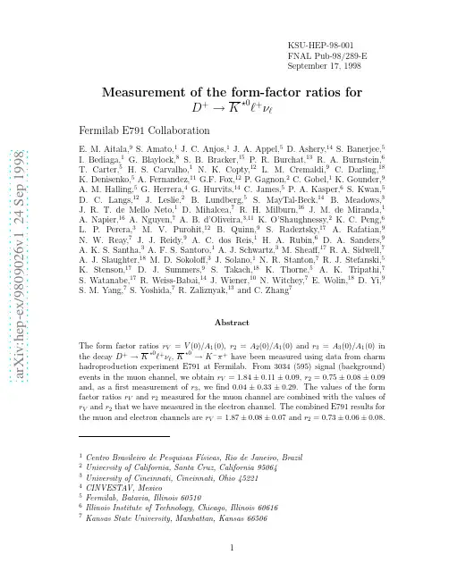
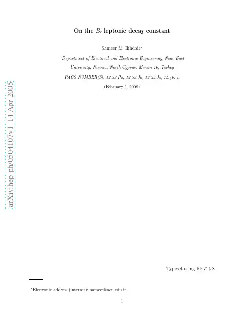
a r X i v :h e p -e x /9809026v 1 24 S e p 1998KSU-HEP-98-001FNAL Pub-98/289-E September 17,1998Measurement of the form-factor ratios forD +→K⋆0ℓ+νℓ,1Centro Brasileiro de Pesquisas F´ısicas,Rio de Janeiro,Brazil 2University of California,Santa Cruz,California 950643University of Cincinnati,Cincinnati,Ohio 452214CINVESTAV,Mexico5Fermilab,Batavia,Illinois 605106Illinois Institute of Technology,Chicago,Illinois 606167Kansas State University,Manhattan,Kansas 665068University of Massachusetts,Amherst,Massachusetts010039University of Mississippi,University,Mississippi3867710Princeton University,Princeton,New Jersey0854411Universidad Autonoma de Puebla,Mexico12University of South Carolina,Columbia,South Carolina2920813Stanford University,Stanford,California9430514Tel Aviv University,Tel Aviv,Israel15Box1290,Enderby,BC,V0E1V0,Canada16Tufts University,Medford,Massachusetts0215517University of Wisconsin,Madison,Wisconsin5370618Yale University,New Haven,Connecticut06511K⋆0ℓ+νℓare an especially clean way to study these effects because the leptonicand hadronic currents completely factorize in the decay amplitude.All informa-tion about the strong interactions can be parametrized by a few form factors.Also, according to Heavy Quark Effective Theory,the values of form factors for somesemileptonic charm decays can be related to those governing certain b-quark de-cays.In particular,the form factors studied here can be related to those for therare B–meson decays B→K⋆e+e−and B→K⋆γ[1,2]which provide windows for physics beyond the Standard Model.With a vector meson in thefinal state,there are four form factors,V(q2),A1(q2),A2(q2)and A3(q2),which are functions of the Lorentz-invariant momentum transfer squared[3].The differential decay rate for D+→K⋆0→K−π+is a quadratic homogeneous function of the four form factors.Unfortunately,the limited size of current data samples precludes precise measurement of the q2-dependence of the form factors;we thus assume the dependence to be given by the nearest-pole dominance model:F(q2)=F(0)/(1−q2/m2pole)where m pole= m V=2.1GeV/c2for the vector form factor V,and m pole=m A=2.5GeV/c2 for the three axial-vector form factors[4].The third form factor A3(q2),which is unobservable in the limit of vanishing lepton mass,probes the spin-0component of the off-shell W.Additional spin-flip amplitudes,suppressed by an overall factor of m2ℓ/q2when compared with spin no-flip amplitudes,contribute to the differential decay rate.Because A1(q2)appears among the coefficients of every term in the differential decay rate,it is customary to factor out A1(0)and to measure the ratios r V=V(0)/A1(0),r2=A2(0)/A1(0)and r3=A3(0)/A1(0).The values of these ratios can be extracted without any assumption about the total decay rate or the weak mixing matrix element V cs.We report new measurements of the form factor ratios for the muon chan-nel and combine them with slightly revised values of our previously publishedmeasurements of r V and r2[5]for the electron channel.This is thefirst set of measurements in both muon and electron channels from a single experiment.We also report thefirst measurement of r3=A3(0)/A1(0),which is unobservable in the limit of vanishing charged lepton mass.E791is afixed-target charm hadroproduction experiment[6].Charm particles were produced in the collisions of a500GeV/cπ−beam withfive thin targets, one platinum and four diamond.About2×1010events were recorded during the 1991-1992Fermilabfixed-target run.The tracking system consisted of23planes of silicon microstrip detectors,45planes of drift and proportional wire chambers, and two large-aperture dipole magnets.Hadron identification is based on the in-formation from two multicellˇCerenkov counters that provided good discrimination between kaons and pions in the momentum range6−36GeV/c.In this momentum range,the probabability of misidentifying a pion as a kaon depends on momentum but does not exceed5%.We identified muon candidates using a single plane of scintillator strips,oriented horizontally,located behind an equivalent of2.4meters of iron(comprising the calorimeters and one meter of bulk steel shielding).The an-gular acceptance of the scintillator plane was≈±62mrad×±48mrad(horizontally and vertically,respectively),which is somewhat smaller than that of the rest of the spectrometer for tracks which go through both magnets(≈±100mrad×±64mrad). The vertical position of a hit was determined from the strip’s vertical position,and the horizontal position of a hit from timing information.The event selection criteria used for this analysis are the same as for the electronic-mode form factor analysis[5],except for those related to lepton identifi-cation.Events are selected if they contain an acceptable decay vertex determined by the intersection point of three tracks that have been identified as a muon,a kaon,and a pion.The longitudinal separation between this candidate decay vertex and the reconstructed production vertex is required to be at least15times the esti-mated error on the separation.The two hadrons must have opposite charge.If the kaon and the muon have opposite charge,the event is assigned to the“right-sign”sample;if they have the same charge,the event is assigned to the“wrong-sign”sample used to model the background.To reduce the contamination from hadron decays inflight,only muon can-didates with momenta larger than8GeV/c are retained.With this momentum restriction,the efficiency of muon tagging was about85%,and the probability for a hadron to be identified as a muon was about3%.To exclude feedthrough from D+→K−π+π+,we exclude events in which the invariant mass of the three charged particles(with the muon candidate interpreted as a pion)is consistent with the D+mass.For ourfinal selection criteria,we use a binary-decision-tree algorithm(CART[7]),whichfinds linear combinations of parameters that have the highest discrimination power between signal and ing this algorithm,we found a linear combination of four discrimination variables[5]:(a)separation significance of the candidate decay vertex from target material;(b)distance of closest approach of the candidate D momentum vector to the primary vertex,taking into account the maximum kinematically-allowedmiss distance due to the unobserved neutrino;(c)product over candidate D decay tracks of the distance of closest approach of the track to the secondary vertex, divided by the distance of closest approach to the primary vertex,where each dis-tance is measured in units of measurement errors;and(d)significance of separation between the production and decay vertices.Thisfinal selection criterion reduced the number of wrong-sign events by50%,and the number of right-sign events by 25%.Although this does not affect our sensitivity substantially,it does reduce systematic uncertainties associated with the background subtraction.The minimum parent mass M min is defined as the invariant mass of Kπµνwhen the neutrino momentum component along the D+direction offlight is ignored.The distribution of M min should have a Jacobian peak at the D+mass,and we observe such a peak in our data(Fig.1).We retain events with M min in the range1.6 to2.0GeV/c2as indicated by the arrows in thefigure.The distribution of Kπinvariant mass for the retained events is shown in the top right of Fig.1for both right-sign and wrong-sign samples.Candidates with0.85<M Kπ<0.94GeV/c2 were retained,yieldingfinal data samples of3629right-sign and595wrong-sign events.The hadroproduction of charm,the differential decay rate,and the detector response were simulated with a Monte Carlo event generator.A sample of events was generated according to the differential decay rate(Eq.22in Ref.[3]),with the form factor ratios r V=2.00,r2=0.82,and r3=0.00.The same selection criteria were applied to the Monte Carlo events as to real data.Out of25million generated events,95579decays passed all cuts.Figure1(bottom)shows the distribution of M Kπfrom real data after background subtraction(“right-sign”minus“wrong-sign”)overlaid with the corresponding Monte Carlo distribution after all cuts are applied.The agreement between the two distributions suggests that wrong-sign events correctly account for the size of the background.The differential decay rate[3]is expressed in terms of four independent kine-matic variables:the square of the momentum transfer(q2),the polar angleθV in theK⋆0and W+decay planes.The definition we use for the polar angle θℓis related to the definition used in Ref.[3]byθℓ→π−θℓ.Semileptonic decays cannot be fully reconstructed due to the undetected neu-trino.With the available information about the D+direction offlight and the charged daughter particle momenta,the neutrino momentum(and all the decay’s kinematic variables)can be determined up to a two-fold ambiguity if the parent mass is constrained.Monte Carlo studies show that the differential decay rate is more accurately determined if it is calculated with the solution corresponding to the lower laboratory-frame neutrino momentum.To extract the form factor ratios the distribution of the data points in the four-dimensional kinematic variable space isfit to the full expression for the differential decay rate.We use the same unbinned maximum-likelihoodfitting technique as inour D+→K⋆0µ+νµcandidates as the previous method, but uses additional neutrino-momentum solutions.This is true for both the data and for the Monte Carlo sample used in the likelihood function calculation,so the results of thisfit could differ from those of the previousfit.The values of the form factor ratios obtained with the two methods agree well, providing further assurance that selecting the lower neutrino momentum solution in the primary method and correcting for the systematic bias gives the correct result.However,the systematic uncertainties for the primary method(see below) were found to be significantly smaller,mainly because the unbinned maximum-likelihood method is more stable against changes in the size of the phase spacevolume.Therefore,the primary method was chosen for quotingfinal results.We classify systematic uncertainties into three categories:(a)Monte Carlo simulation of detector effects and production mechanism;(b)fitting technique;(c) background subtraction.The estimated contributions of each are given in Table I. The main contributions to category(a)are due to muon identification and data selection criteria.The contributions to category(b)are related to the limited size of the Monte Carlo sample and to corrections for systematic bias.The measurements of the form factor ratios for D+→K⋆0e+νe[5]follow the same analysis procedure except for the charged lepton identification.Both results are listed in Table II.The consistency within errors of the results measured in the electron and muon channels supports the assumption that strong interaction effects,incor-porated in the values of form factor ratios,do not depend on the particular W+ leptonic decay.Based on this assumption,we combine the results measured for the electronic and muonic decay modes.The averaged values of the form factor ratios are r V=1.87±0.08±0.07and r2=0.73±0.06±0.08.The statistical and systematic uncertainties of the average results were determined using the general procedure described in Ref.[9](Eqns.3.40and3.40′).Some of the systematic errors for the two samples have positive correlation coefficients,and some nega-tive.The combination of all systematic errors is ultimately close to that which one would obtain assuming all the errors are uncorrelated.The third form factor ratio r3was not measured in the electronic mode.Table II compares the values of the form factor ratios r V and r2measured by E791in the electron,muon and combined modes with previous experimental results.The size of the data sample and the decay channel are listed for each case. All experimental results are consistent within errors.The comparison between the E791combined values of the form factor ratios r V and r2and previous experimental results is also shown in Fig.3(top).Table III and Fig.3(bottom)compare thefinal E791result with published theoretical predictions.The spread in the theoretical results is significantly larger than the E791experimental errors.To summarize,we have measured the values of the form factor ratios in the decay channel D+→K⋆0e+νe gives r V=1.87±0.08±0.07and r2=0.73±0.06±0.08.We gratefully acknowledge the assistance from Fermilab and other participat-ing institutions.This work was supported by the Brazilian Conselho Nacional de Desenvolvimento Cient´ıfico e Technol´o gico,CONACyT(Mexico),the Israeli Academy of Sciences and Humanities,the U.S.Departament of Energy,the U.S.-Israel Binational Science Foundation,and the U.S.National Science Foundation.REFERENCES[1]N.Isgur and M.B.Wise,Phys.Rev.D42(1990)2388.[2]Z.Ligeti,I.W.Stewart and M.B.Wise,Phys.Lett.B420(1998)359.[3]J.G.K¨o rner and G.A.Schuler,Phys.Lett.B226(1989)185.[4]Particle Data Group,Review of Particle Physics,Phys.Rev.D50(1994)1568.[5]Fermilab E791Collaboration,E.M.Aitala et al.,Phys.Rev.Lett.80(1998)1393.The E791electron result for r V quoted in this paper is0.06higher than the value reported in this reference because we have corrected for inaccuracies in the earlier modeling of the D+transverse momentum.[6]J.A.Appel,Ann.Rev.Nucl.Part.Sci.42(1992)367;D.J.Summers et al.,XXVII Rencontre de Moriond,Les Arcs,France(15-22March1992)417. [7]L.Brieman et al.,Classification and Regression Trees(Chapman and Hall,New York,1984).[8]D.M.Schmidt,R.J.Morrison,and M.S.Witherell,Nucl.Instrum.Methods A328(1993)547.[9]L.Lyons,Statistics for Nuclear and Particle Physicists(Cambridge UniversityPress,Cambridge,1986).[10]Fermilab E687Collaboration,P.L.Frabetti et al.,Phys.Lett.B307(1993)262.[11]Fermilab E653Collaboration,K.Kodama et al.,Phys.Lett.B274(1992)246.[12]Fermilab E691Collaboration,J.C.Anjos et al.,Phys.Rev.Lett.65(1990)2630.[13]D.Scora and N.Isgur,Phys.Rev.D52(1995)2783.We have used the q2-dependence assumed in thefits to our data to extrapolate the theoretical form factors from q2=q2max to q2=0.[14]M.Wirbel,B.Stech,and M.Bauer,Z.Phys.C29(1985)637.[15]T.Altomari and L.Wolfenstein,Phys.Rev.D37(1988)681.[16]F.J.Gilman and R.L.Singleton,Jr.,Phys.Rev.D41(1990)142.[17]B.Stech,Z.Phys.C75(1997)245.[18]C.W.Bernard,Z.X.El-Khadra,and A.Soni,Phys.Rev.D45(1992)869,Phys.Rev.D47(1993)998.[19]V.Lubicz,G.Martinelli,M.S.McCarthy,and C.T.Sachrajda,Phys.Lett.B274(1992)415.[20]A.Abada et al.,Nucl.Phys.B416(1994)675.[21]C.R.Alton et al.,Phys.Lett.B345(1995)513.[22]K.C.Bowler et al.,Phys.Rev.D51(1995)4905.[23]P.Ball,V.M.Braun,and H.G.Dosch,Phys.Rev.D44(1991)3567.[24]T.Bhattacharya and R.Gupta,Nucl.Phys.B(Proc.Suppl.)47(1996)481.TABLESTABLE I.The main contributions to uncertainties on the form factor ratios.Sourceσr2σrVσr3Hadron identification0.010.010.02 Muon identification0.040.060.10 Production mechanism0.010.010.02 Acceptance0.030.020.08 Cut selection0.030.040.09MC volume size0.020.020.12 Number of MC points0.010.010.18 Bias0.010.020.06No.of background events0.040.020.06 Background shape0.040.040.06 E7916000(e+µ)1.87±0.08±0.070.73±0.06±0.08 E7913000(µ)1.84±0.11±0.090.75±0.08±0.09 E7913000(e)1.90±0.11±0.090.71±0.08±0.09 E687[10]900(µ)1.74±0.27±0.280.78±0.18±0.10E653[11]300(µ)2.00+0.34−0.32±0.160.82+0.22−0.23±0.11E691[12]200(e)2.0±0.6±0.30.0±0.5±0.2TABLE parison of E791results with theoretical predictions for the form factor ratios r V and r2.Group r V r2ISGW2[13]2.01.3WSB[14]1.41.3KS[3]1.01.0AW/GS[15,16]2.00.8Stech[17]1.551.06BKS[18]1.99±0.22±0.330.70±0.16±0.17 LMMS[19]1.6±0.20.4±0.4ELC[20]1.3±0.20.6±0.3APE[21]1.6±0.30.7±0.4UKQCD[22]1.4+0.5−0.20.9±0.2BBD[23]2.2±0.21.2±0.2 LANL[24]1.78±0.070.68±0.11FIGURES01002003004005006001.251.51.7522.25M min (GeV/ c 2)E v e n t s / 40 M e V / c21002003004005006007000.70.80.91 1.1K π invariant mass (GeV/ c 2)E v e n t s / 10 M e V / c 2050100150200250300K π invariant mass (GeV/ c 2)E v e n t s / 5 M e V / c2FIG.1.Distributions of minimum parent mass M min and Kπinvariant mass for D +→050100150200cos θl (q 2/q 2max < 0.5)E v e n t s / 0.2050100150200cos θl (q 2/q 2max ≥ 0.5)E v e n t s / 0.250100150200cos θV (q 2/q 2max < 0.5)E v e n t s / 0.2050100150200cos θV (q 2/q 2max ≥ 0.5)E v e n t s / 0.250100150200χ (cos θV < 0)E v e n t s / 0.2π050100150200χ (cos θV ≥ 0)E v e n t s / 0.2πparison of single-variable distributions of background-subtracted data (crosses)with Monte Carlo predictions (dashed histograms)using best-fit values for the form factor ratios.1111.21.41.61.822.22.4rr V11.21.41.61.822.22.4r 2r VFIG.3.Top:Comparison of experimental measurements of form factor ratios r V and r 2for D +→。
Masses and decay constants of B_q mesons in the QCD string approach
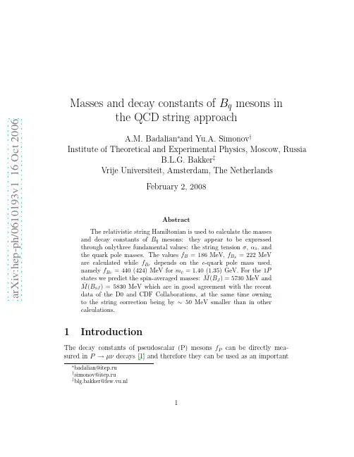
a rXiv:h ep-ph/61193v116Oct26Masses and decay constants of B q mesons in the QCD string approach A.M.Badalian ∗and Yu.A.Simonov †Institute of Theoretical and Experimental Physics,Moscow,Russia B.L.G.Bakker ‡Vrije Universiteit,Amsterdam,The Netherlands February 2,2008Abstract The relativistic string Hamiltonian is used to calculate the masses and decay constants of B q mesons:they appear to be expressed through onlythree fundamental values:the string tension σ,αs ,and the quark pole masses.The values f B =186MeV,f B s =222MeV are calculated while f B c depends on the c -quark pole mass used,namely f B c =440(424)MeV for m c =1.40(1.35)GeV.For the 1P states we predict the spin-averaged masses:¯M (B J )=5730MeV and ¯M (B sJ )=5830MeV which are in good agreement with the recent data of the D0and CDF Collaborations,at the same time owningto the string correction being by ∼50MeV smaller than in other calculations.1IntroductionThe decay constants of pseudoscalar (P)mesons f P can be directly mea-sured in P →µνdecays [1]and therefore they can be used as an importantcriterium to compare different theoretical approaches and estimate their ac-curacy.Although during the last decade f P were calculated many times:in potential models[2,3,4],the QCD sum rule method[5],and in lattice QCD [6,7],here we again address the properties of the B,B s,B c mesons for several reasons.First,we use here the relativistic string Hamiltonian(RSH)[8],which is derived from the QCD Lagrangian with the use of thefield correlator method (FCM)[9]and successfully applied to light mesons and heavy quarkonia [10,11].Here we show that the meson Green’s function and decay constants can also be derived with the use of FCM.Second,the remarkable feature of the RSH H R and also the correlator of the currents G(x)is that they are fully determined by a minimal number of fundamental parameters:the string tensionσ,ΛMS=250(5)MeV;(1) and the pole masses taken arem u(d)=0;m s=170(10)MeV;m c=1.40GeV;m b=4.84GeV.(2) Third,recently new data on the masses of B c and the P-wave mesons: B1,B2,and B s2have been reported by the D0and CDF Collaborations [12,13],which give additional information on the B q-meson spectra.Here we calculate the spin-averaged masses of the P-wave states B and B s.We would like to emphasize here that in our relativistic calculations no constituent masses are used.In the meson mass formula an overall(fitting) constant,characteristic for potential models,is absent and the whole scheme appears to be rigid.Nevertheless,we take into account an important nonperturbative(NP) self-energy contribution to the quark mass,∆SE(q)(see below eq.(18)).For the heavy b quark∆SE(b)=0and for the c quark∆SE(c)≃−20MeV[10], which is also small.For any kind of mesons we use a universal static potential with pure scalarconfining term,V0(r)=σr−4r,(3)2where the couplingαB(r)possesses the asymptotic freedom property and saturates at large distances withαcrit(n f=4)=0.52[14].The coupling can be expressed throughαB(q)in momentum space,αB(r)=2qαB(q),(4)whereαB(q)=4πβ20ln t BΛ2B.Here the QCD constantΛB,is expressed as[15]ΛB(n f)=Λ2β0· 319n f (6)and M B(σ,ΛB)=(1.00±0.05)GeV is the so called background mass[14]. For heavy-light mesons withΛ2+m2i+p2In (8)m 1(m 2)is the pole (current)mass of a quark (antiquark).The variable ωi is defined from extremum condition,which is taken either from(1)The exact condition:∂H 0p 2+m 2i .(10)ThenH 0ϕn = p 2+m 22+V 0(r ) ϕn =M n ϕn(11)reduces to the Salpeter equation,which just defines ωi (n )=∂˜ωi =0(the so-called einbein approxima-tion).As shown in [9]the difference between ωi and ˜ωi is <∼5%.For the RSH (7)the spin-averaged massM (nL )=ω12+m 212ωb +E n (µ)−2σηf p 2+m 2i nL ;µ=ω1ωbπωf ;(14)with ηf =0.9for a u (d )quark,ηf ∼=0.7for an s quark,ηf =0.4for a c quark,and ηb =0.Therefore,for a b quark ∆SE (b )=0.The mass formula(12)does not contain any overall constant C .Note that the presence of C violates linear behavior of Regge trajectories.The calculated masses of the low-lying states of B ,B s ,and B c mesons are given in Table 2,as well as their values taken from [2,3,6,7].It is of interest to notice that in our calculations the masses of the P -wave states appear to be by 30-70MeV lower than in [2]due to taking into account a string correction [11].4Table1:Masses of the low-lying B q mesons in the QCD String Approach B5280(5)a5279.0(5)5310252753B1(1P)¯M=5730a5721(8)D05734(5)CDFB s5369a5369.6(24)5390253623B s2¯M=58305839(3)D058802B∗c6330(5)a633826321(20)63Current CorrelatorThe FCM can be also used to define the correlator GΓ(x)of the currents jΓ(x),jΓ(x)=¯ψ1(x)Γψ2(x),(15) for S,P,V,and A channels(here the operatorΓ=t a⊗(1,γ5,γµ,iγµγ5)).The correlator,GΓ(x)≡ jΓ(x)jΓ(0) vac,(16) with the use of spectral decomposition of the currents jΓand the definition, vac|¯ψ1γ0γ5ψ2|P n(k=0) =f P n M n,(A,P)vac|¯ψ1γµψ2|V n(k,ε) =f V n M nεµ,(V)(17) can be presented as[3]GΓ(x)d x= n M n0|YΓe−H0T|0ω1ω2N c YΓ=p2 .(20)3Then from Eqs.(18)and(19)one obtains the following analytical expression for the decay constants(for a given state labelled n):f P(V)n 2=2N c M n|ϕn(0)|2.(21)This very transparent formula contains only well defined factors:ω1andωb, the meson mass M n,andϕn the eigenvector ofˆH0.Then in the P channelf P n 2=6(m1m2+ω1ω2− p2 )Table2:Pseudoscalar constants of B q mesons(in MeV)f B189216(34)186(5)f B s218249(42)222(2)f B swhere the w.f.at the origin,ϕn(0),is a relativistic one.In the nonrelativistic limitωi→m i,ϕn(0)→ϕNR n(0)and one comes to the standard expression:f P n(0) 2→12•In our analytic approach with minimal input of fundamental parame-ters(σ,αs,m i)the calculated decay constants are f B=186MeV,f B s=222MeV,f B s/f B=1.19.•For B c the decay constant is very sensitive to m c(pole):f B c=440MeV(m c=1.40GeV)and f B c=425MeV(m c=1.35GeV)References[1]D.Silverman and H.Yao,Phys.Rev.D38,214(1988).[2]S.Godfrey and N.Isgur,Phys.Rev.D32,189(1985);S.Godfrey,Phys.Rev.D70,054017(2004).[3]D.Ebert,R.N.Faustov,and V.O.Galkin,hep-ph/0602110;Mod.Phys.Lett.A17,803(2002),and references therein.[4]G.Cvetic,C.S.Kim,G.L.Wang,and W.K.Namgung,Phys.Lett.B596,84(2004).[5]M.Jamin,nge,Phys.Rev.D65,056005(2002)and referencestherein.[6]A.Ali Khan et al.,Phys.Rev.D70,114501(2004),ibid.64,054504(2004);C.T.H.Davies et al.,Phys.Rev.Lett.92,022001(2004).[7]A.S.Kronfeld,hep-lat/0607011and references therein;I.F.Allison etal.,Phys Rev.Lett.94172001(2005);A.Gray et al.,Phys.Rev.Lett.95,212001(2005).[8]A.Yu.Dubin,A.B.Kaidalov,and Yu.A.Simonov,Phys.Lett.B323,41(1994);Phys.Atom Nucl.56,1745(1993);E.L.Gubankova and A.Yu.Dubin,Phys.Lett.B334,180(1994).[9]H.G.Dosch and Yu.A.Simonov,Phys.Lett.B205,339(1988);Yu.A.Simonov,Z.Phys.C53,419(1992);Yu.S.Kalashnikova,A.V.Nefediev,and Yu.A.Simonov,Phys.Rev.D64,014037(2001);Yu.A.Simonov,Phys.Atom.Nucl.67,553(2004).[10]A.M.Badalian,A.I.Veselov,and B.L.G.Bakker,Phys.Rev.D70,016007(2004);Phys.Atom.Nucl.67,1367(2004).8[11]A.M.Badalian and B.L.G.Bakker,Phys.Rev.D66,034025(2002);A.M.Badalian,B.L.G.Bakker,and Yu.A.Simonov,Phys.Rev.D66,034025(2002).[12]P.Catastini(for the D0and CDF Collab.),hep-ex/0605051;M.D.Cor-coran,hep-ex/0506061.[13]D.Acosta et al.(CDF Collab.),Phys.Rev.Lett.96,202001(2006);hep-ex/0508022.[14]A.M.Badalian and D.S.Kuzmenko,Phys.Rev.D65,016004(2002);A.M.Badalian and Yu.A.Simonov,Phys.Atom.Nucl.60,636(1997).[15]M.Peter,Phys.Rev.Lett.76,602(1997);Y.Schr¨o der,Phys.Lett.B447,321(1999).[16]Yu.A.Simonov,Phys.Lett.B515,137(2001).[17]Particle Data Group,S.Eidelman,et al.,Phys.Lett.B592,1(2004).[18]A.M.Badalian and Yu.A.Simonov(in preparation).9。
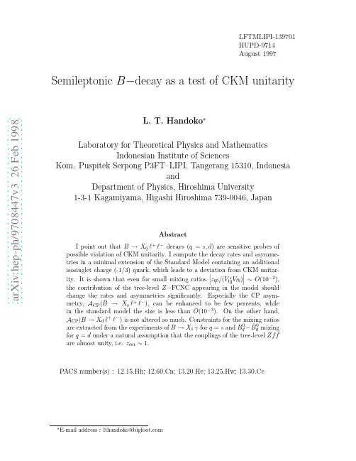
Semileptonic B decay as a test of CKM unitarity
U u ij 0 0 U d αβ
uj dβ
.
weak
(5)
Indeed, using the unitarityty violation in the present interest can be expressed as follows,
(7)
where q µ denotes four-momentum of the dilepton and s = q 2 . Notations with hat on the top means it is normalized with the b−quark mass. In the tree-level approximation, new interactions in Eq. (2) contributes to O9 and O10 . Therefore, involving the continuum and resonances parts into calculation gives
Abstract I point out that B → Xq ℓ+ ℓ− decays (q = s, d) are sensitive probes of possible violation of CKM unitarity. I compute the decay rates and asymmetries in a minimal extension of the Standard Model containing an additional isosinglet charge (-1/3) quark, which leads to a deviation from CKM unitar∗ V ) ∼ O (10−2 ), ity. It is shown that even for small mixing ratios zqb /(Vtq tb the contribution of the tree-level Z −FCNC appearing in the model should change the rates and asymmetries significantly. Especially the CP asymmetry, ACP (B → Xs ℓ+ ℓ− ), can be enhanced to be few percents, while in the standard model the size is less than O(10−3 ). On the other hand, ACP (B → Xd ℓ+ ℓ− ) is not altered so much. Constraints for the mixing ratios 0 −B ¯ 0 mixing are extracted from the experiments of B → Xs γ for q = s and Bd d ¯ for q = d under a natural assumption that the couplings of the tree-level Zf f are almost unity, i.e. zαα ∼ 1.
Twist-3 distribution amplitudes of scalar mesons from QCD sum rules
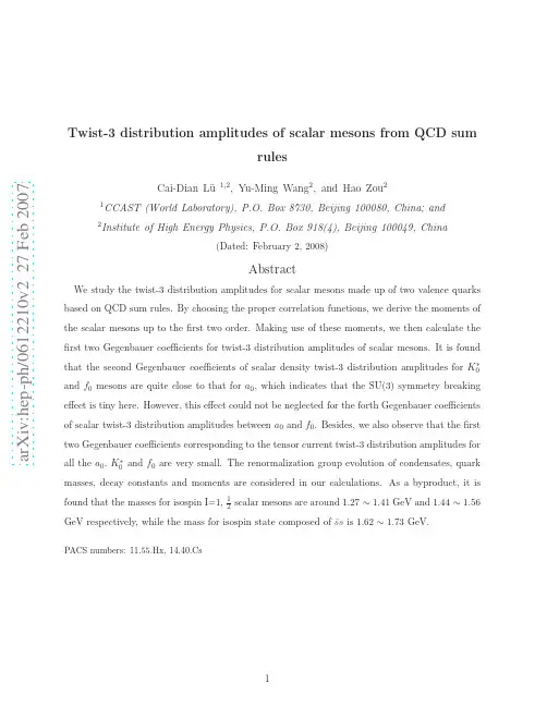
that the second Gegenbauer coefficients of scalar density twist-3 distribution amplitudes for K0∗ and f0 mesons are quite close to that for a0, which indicates that the SU(3) symmetry breaking effect is tiny here. However, this effect could not be neglected for the forth Gegenbauer coefficients
found
that
the
masses
for
isospin
I=1,
1 2
scalar
mesons
are
around
1.27
∼
1.41
GeV
and
1.44
∼
1.56
GeV respectively, while the mass for isospin state composed of s¯s is 1.62 ∼ 1.73 GeV.
2
moments for the above three scalar mesons in section III. The last section is devoted to our conclusions.
II. FORMULATION
In the valence quark model, there are two twist-3 light-cone distribution amplitudes for scalar mesons which are defined as [6]
On the B_{c} leptonic decay constant
Sameer M. Ikhdair∗
∗ Department
of Electrical and Electronic Engineerinsity, Nicosia, North Cyprus, Mersin-10, Turkey PACS NUMBER(S): 12.39.Pn, 12.39.Jh, 13.25.Jx, 14.40.-n
arXiv:hep-ph/0504107v1 14 Apr 2005
(February 2, 2008)
Typeset using REVTEX
∗ Electronic
address (internet): sameer@.tr
1
Abstract
We give a review and present a comprehensive calculations for the leptonic constant fBc of the low-lying pseudoscalar and vector states of Bc -meson in the framework of static and QCD-motivated nonrelativistic potential models taking into account the one-loop and two-loop QCD corrections in the short distance coefficient that governs the leptonic constant of Bc quarkonium system. Further, we use the scaling relation to predict the leptonic constant of the nS-states of the bc system. Our results are compared with other models to gauge the reliability of the predictions and point out differences.
Decay Constants $f_{D_s^}$ and $f_{D_s}$ from ${bar{B}}^0to D^+ l^- {bar{nu}}$ and ${bar{B}
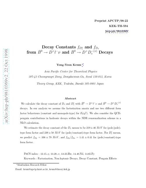
form factor.
PACS index : 12.15.-y, 13.20.-v, 13.25.Hw, 14.40.Nd, 14.65.Fy Keywards : Factorization, Non-leptonic Decays, Decay Constant, Penguin Effects
∗ experimentally from leptonic B and Ds decays. For instance, determine fB , fBs fDs and fDs
+ the decay rate for Ds is given by [1]
+ Γ(Ds
m2 G2 2 2 l 1 − m M → ℓ ν ) = F fD D s 2 8π s ℓ MD s
1/2
(4)
.
(5)
In the zero lepton-mass limit, 0 ≤ q 2 ≤ (mB − mD )2 .
2
For the q 2 dependence of the form factors, Wirbel et al. [8] assumed a simple pole formula for both F1 (q 2 ) and F0 (q 2 ) (we designate this scenario ’pole/pole’): q2 F1 (q ) = F1 (0) /(1 − 2 ), mF1
∗ amount to about 11 % for B → DDs and 5 % for B → DDs , which have been mentioned in
Heavy-light decay constants with three dynamical flavors
light quark masses, the chiral extrapolation was
a major source of systematic error. Here, chang-
ing from linear to quadratic chiral fits of decay constants changes the results by <∼2%.
quette following Refs. [3,11], and then define the 1-loop coefficient ζA by ZAtad = 1 + αPs ζA.
(2) Fix the scale from mρ on each set, with valence quarks extrapolated to physical values.
∞/∞
8.40 0.09 417 200
0.031/0.031 7.18 0.09 162 40
0.0124/0.031 7.11 0.09 25 –
tors for 5 light and 5 heavy masses. This gives
good control over both chiral and heavy quark
We present preliminary results for the heavy-light leptonic decay constants in the presence of three light dynamical flavors. We generate dynamical configurations with improved staggered and gauge actions and analyze them for heavy-light physics with tadpole improved clover valence quarks. When the scale is set by mρ, we find an increase of ≈ 23% in fB with three dynamical flavors over the quenched case. Discretization errors appear to be small (<∼3%) in the quenched case but have not yet been measured in the dynamical case.
Charmless Three-body Decays of B Mesons
Abstract
An exploratory study of charmless 3-body decays of B mesons is presented using a simple model based on the framework of the factorization approach. The nonresonant contributions arising from B → P1 P2 transitions are evaluated using heavy meson chiral perturbation theory (HMChPT). The momentum dependence of nonresonant amplitudes is assumed to be in the exponential form e−αNR pB ·(pi +pj ) so that the HMChPT results are recovered in the soft meson limit pi , pj → 0. In addition, we have identified another large source of the nonresonant signal in the matrix elements 0 of scalar densities, e.g. KK |s ¯s|0 , which can be constrained from the decay B → KS KS KS or B − → K − KS KS . The intermediate vector meson contributions to 3-body decays are identified through the vector current, while the scalar meson resonances are mainly associated with the scalar density. Their effects are described in terms of the Breit-Wigner formalism. Our main results are: (i) All KKK modes are dominated by the nonresonant background. The predicted branching ratios of K + K − KS (L) , K + K − K − and K − KS KS modes are consistent with the data within errors. (ii) Although the penguin-dominated B 0 → K + K − KS decay is subject to a potentially significant tree pollution, its effective sin 2β is very similar to that of the KS KS KS mode. However, direct CP asymmetry of the former, being of order −4%, is more prominent than the latter. (iii) For 0 B → Kππ decays, we found sizable nonresonant contributions in K − π + π − and K π + π − modes, in agreement with the Belle measurements but larger than the BaBar result. (iv) Time-dependent CP asymmetries in KS π 0 π 0 , a purely CP -even state, and KS π + π − , an admixture of CP -even and CP -odd components, are studied. (v) The π + π − π 0 mode is found to have a rate larger than π + π − π − even though the former involves a π 0 in the final state. They are both dominated by resonant ρ contributions. (vi) We have computed the resonant contributions to 3-body decays and determined the rates for the quasi-two-body decays B → V P and B → SP . The predicted ρπ, f0 (980)K and f0 (980)π rates are in agreement with the data, while the calculated φK, K ∗ π, ρK ∗ (1430)π are in general too small compared to experiment. (vii) Sizable direct CP asymmetry and K0 is found in K + K − K − and K + K − π − modes.
Dielectric_constant
Properties of microwave dielectricsIn microwave technique, a large variety of materials are used, includingdielectrics. The measurement of the dielectric properties of microwave materials isnot only helpful in understanding the structural information and studying themicrowave characteristics but also designing microwave devices. The aim of thisexperiment is to understand the property of resonant cavities, and to learn theprinciple and method for measuring the complex dielectric constant of materials.1.PrincipleAccording to the theory of electromagnetic field, a dielectric in alternatingelectric field will be rotational polarized, and it relaxes during the polarization. So itsdielectric constant is a complex number, which can be expressed as follows:"'εεεj r -=where ε’ and ε” are the real part and imagine part of the complex dielectric constant.Due to relaxation of the dielectric in alternating electric field, the electricdisplacement vector in the dielectric has a phase hysteresis of an angel δ in respectiveto that outside the dielectric. The phase angle δ can be calculated from the followingequation:.'"εεδ=tg tgδ is called the dissipation factor or tangent-of-dissipation-angle, because the energydissipation in dielectrics is proportional to tgδ.Selecting a TE 10n rectangle resonant cavity with n an old number, generally takento be 3, and make a small hole at the center (x=a /2, z=l /2), where the electric field ismaximal, and magnetic field is minimal. The dielectric to be measured is processed tobe a long and thin rod, and inserted into thecavity through the small hole.As the dielectric rod is very small, thedistribution of the electromagnetic field in thewhole cavity is kept almost unchanged exceptnear the dielectric rod. Therefore the dielectricrod can be regarded as a micro disturbance tothe field distribution of the cavity. Accordingto the theory of micro disturbance of resonant cavity, one obtains [1]:ss V V f f f 000211'-+=εss V V Q Q 001141"⎪⎪⎭⎫ ⎝⎛-=εwhere V 0 and V s are the volumeof the cavity and that of thedielectric rod, respectively. f oand Q 0 are the resonantfrequency and quality factor ofthe cavity without the dielectric,and f s and Q s are that with thedielectric. The quality factor fora resonant cavity can becalculatedfromfollowing equation:hf f Q ∆=0where Δf h is the half-power frequency width of the resonant curve (Fig.1). Usingreflecting cavity as the sample cavity, then the complex dielectric constant canbeFig.1 The sample cavityFig.2 The resonant curve of a reflection cavitycalculated by measuring the resonant frequency f0 and half-power frequency width Δf h.2. Apparatus and InstrumentationThe experimental apparatus for the measurement of the complex dielectric constant is shown in Fig.3. The klystron working at sawtooth-wave-modulation mode,Fig.3 The experimental setup for dielectric constant measurementoutput a frequency-modulated microwave. The isolator is a single direction device. Microwave power is only transmitted in the direction of the arrow, and waves reflected back towards the klystron are attenuated. The function of the attenuator is to adjust the microwave power. The frequency meter is a cavity, which absorbs microwave in a narrow band. If the band absorbed by the meter, is within the frequency range generated by the klystron, a dip will appear in the oscilloscope displayer of microwave power vs. frequency. The circulator is a kind of power divider. It divides the input power into two parts. One part is transmitted in the sample cavity, and the other in the isolator. The microwave power through the isolator is detected by a crystal detector, and the voltage pulse proportional to the power is then observed in the oscilloscope.3. Contents of the experiment3.1 Observations of the vibration modulus of the klystron with oscilloscope(1)Make the sample cavity non-resonant, through adjusting the frequency ofmicrowave from the klystron by mechanical tuning;(2)Adjust the reflector voltage, and observe the vibration modulus of the klystron onthe oscilloscope.3.2 Observations of the resonant curves of the reflecting cavity(1)Make the klystron to work at the best vibration modulus by adjusting the reflectorvoltage;(2)Make the sample cavity to resonate, by changing the microwave frequencythrough mechanical tuning;(3)Observe the resonant curve.3.3 Measurements of the dependences of frequency on time(1)Measure the f ~t curve;(2)Calculate the frequency scale coefficient K at the vicinity of f 0, which isdefined from the equation:.tf K δδ=3.4 Measurements of the complex dielectric constants εr(1)Measure the resonant frequency f 0 and half-power frequency width Δf h0before the insertion of the sample;(2)Measure the resonant frequency f s and half-power frequency width Δf hs afterthe insertion of the sample;(3)Measure the sample volume V s and cavity volume V 0 in mm 3;(4)Calculate the complex dielectric constant.4. Problems(1) What are the characteristic parameters of a resonant cavity?(2) Which parameter of the resonant cavity determines mainly the real part of the complex dielectric constant?References1. 林木欣,能予莹,高长连,朱文钧,刘战存,冯显灿,等,近代物理实验教程,科学出版社,北京,20002.赫崇骏,韩永宁,袁乃昌,何建国,微波电路,国防科技大学出版社,长沙,1999Vocabularycrystal detector 晶体检波器circulator 环行器dissipation factor损耗因子electric displacement vector 电位移矢量energy dissipation能量损耗klystron 速调管mechanical tuning 机械调谐microwave 微波microwave dielectric 微波介质microammeter微安计non-resonant失谐half-power frequency width 半功率频宽half-power frequency 半功率频率hysterisis 滞后oscilloscope 示波器power divider 功率分配器quality factor 品质因素resonant cavity 谐振腔resonant frequency 谐振频率reflecting cavity 反射式腔reflector voltage 反射极电压resonant curve 谐振曲线sawtooth wave锯齿波sample cavity 样品腔tangent of dissipation angle损耗角正切vibration modulus 振荡模。
Principles of Plasma Discharges and Materials Processing9
CHAPTER8MOLECULAR COLLISIONS8.1INTRODUCTIONBasic concepts of gas-phase collisions were introduced in Chapter3,where we described only those processes needed to model the simplest noble gas discharges: electron–atom ionization,excitation,and elastic scattering;and ion–atom elastic scattering and resonant charge transfer.In this chapter we introduce other collisional processes that are central to the description of chemically reactive discharges.These include the dissociation of molecules,the generation and destruction of negative ions,and gas-phase chemical reactions.Whereas the cross sections have been measured reasonably well for the noble gases,with measurements in reasonable agreement with theory,this is not the case for collisions in molecular gases.Hundreds of potentially significant collisional reactions must be examined in simple diatomic gas discharges such as oxygen.For feedstocks such as CF4/O2,SiH4/O2,etc.,the complexity can be overwhelming.Furthermore,even when the significant processes have been identified,most of the cross sections have been neither measured nor calculated. Hence,one must often rely on estimates based on semiempirical or semiclassical methods,or on measurements made on molecules analogous to those of interest. As might be expected,data are most readily available for simple diatomic and polyatomic gases.Principles of Plasma Discharges and Materials Processing,by M.A.Lieberman and A.J.Lichtenberg. ISBN0-471-72001-1Copyright#2005John Wiley&Sons,Inc.235236MOLECULAR COLLISIONS8.2MOLECULAR STRUCTUREThe energy levels for the electronic states of a single atom were described in Chapter3.The energy levels of molecules are more complicated for two reasons. First,molecules have additional vibrational and rotational degrees of freedom due to the motions of their nuclei,with corresponding quantized energies E v and E J. Second,the energy E e of each electronic state depends on the instantaneous con-figuration of the nuclei.For a diatomic molecule,E e depends on a single coordinate R,the spacing between the two nuclei.Since the nuclear motions are slow compared to the electronic motions,the electronic state can be determined for anyfixed spacing.We can therefore represent each quantized electronic level for a frozen set of nuclear positions as a graph of E e versus R,as shown in Figure8.1.For a mole-cule to be stable,the ground(minimum energy)electronic state must have a minimum at some value R1corresponding to the mean intermolecular separation (curve1).In this case,energy must be supplied in order to separate the atoms (R!1).An excited electronic state can either have a minimum( R2for curve2) or not(curve3).Note that R2and R1do not generally coincide.As for atoms, excited states may be short lived(unstable to electric dipole radiation)or may be metastable.Various electronic levels may tend to the same energy in the unbound (R!1)limit. Array FIGURE8.1.Potential energy curves for the electronic states of a diatomic molecule.For diatomic molecules,the electronic states are specifiedfirst by the component (in units of hÀ)L of the total orbital angular momentum along the internuclear axis, with the symbols S,P,D,and F corresponding to L¼0,+1,+2,and+3,in analogy with atomic nomenclature.All but the S states are doubly degenerate in L.For S states,þandÀsuperscripts are often used to denote whether the wave function is symmetric or antisymmetric with respect to reflection at any plane through the internuclear axis.The total electron spin angular momentum S (in units of hÀ)is also specified,with the multiplicity2Sþ1written as a prefixed superscript,as for atomic states.Finally,for homonuclear molecules(H2,N2,O2, etc.)the subscripts g or u are written to denote whether the wave function is sym-metric or antisymmetric with respect to interchange of the nuclei.In this notation, the ground states of H2and N2are both singlets,1Sþg,and that of O2is a triplet,3SÀg .For polyatomic molecules,the electronic energy levels depend on more thanone nuclear coordinate,so Figure8.1must be generalized.Furthermore,since there is generally no axis of symmetry,the states cannot be characterized by the quantum number L,and other naming conventions are used.Such states are often specified empirically through characterization of measured optical emission spectra.Typical spacings of low-lying electronic energy levels range from a few to tens of volts,as for atoms.Vibrational and Rotational MotionsUnfreezing the nuclear vibrational and rotational motions leads to additional quan-tized structure on smaller energy scales,as illustrated in Figure8.2.The simplest (harmonic oscillator)model for the vibration of diatomic molecules leads to equally spaced quantized,nondegenerate energy levelse E v¼hÀv vib vþ1 2(8:2:1)where v¼0,1,2,...is the vibrational quantum number and v vib is the linearized vibration frequency.Fitting a quadratic functione E v¼12k vib(RÀ R)2(8:2:2)near the minimum of a stable energy level curve such as those shown in Figure8.1, we can estimatev vib%k vibm Rmol1=2(8:2:3)where k vib is the“spring constant”and m Rmol is the reduced mass of the AB molecule.The spacing hÀv vib between vibrational energy levels for a low-lying8.2MOLECULAR STRUCTURE237stable electronic state is typically a few tenths of a volt.Hence for molecules in equi-librium at room temperature (0.026V),only the v ¼0level is significantly popula-ted.However,collisional processes can excite strongly nonequilibrium vibrational energy levels.We indicate by the short horizontal line segments in Figure 8.1a few of the vibrational energy levels for the stable electronic states.The length of each segment gives the range of classically allowed vibrational motions.Note that even the ground state (v ¼0)has a finite width D R 1as shown,because from(8.2.1),the v ¼0state has a nonzero vibrational energy 1h Àv vib .The actual separ-ation D R about Rfor the ground state has a Gaussian distribution,and tends toward a distribution peaked at the classical turning points for the vibrational motion as v !1.The vibrational motion becomes anharmonic and the level spa-cings tend to zero as the unbound vibrational energy is approached (E v !D E 1).FIGURE 8.2.Vibrational and rotational levels of two electronic states A and B of a molecule;the three double arrows indicate examples of transitions in the pure rotation spectrum,the rotation–vibration spectrum,and the electronic spectrum (after Herzberg,1971).238MOLECULAR COLLISIONSFor E v.D E1,the vibrational states form a continuum,corresponding to unbound classical motion of the nuclei(breakup of the molecule).For a polyatomic molecule there are many degrees of freedom for vibrational motion,leading to a very compli-cated structure for the vibrational levels.The simplest(dumbbell)model for the rotation of diatomic molecules leads to the nonuniform quantized energy levelse E J¼hÀ22I molJ(Jþ1)(8:2:4)where I mol¼m Rmol R2is the moment of inertia and J¼0,1,2,...is the rotational quantum number.The levels are degenerate,with2Jþ1states for the J th level. The spacing between rotational levels increases with J(see Figure8.2).The spacing between the lowest(J¼0to J¼1)levels typically corresponds to an energy of0.001–0.01V;hence,many low-lying levels are populated in thermal equilibrium at room temperature.Optical EmissionAn excited molecular state can decay to a lower energy state by emission of a photon or by breakup of the molecule.As shown in Figure8.2,the radiation can be emitted by a transition between electronic levels,between vibrational levels of the same electronic state,or between rotational levels of the same electronic and vibrational state;the radiation typically lies within the optical,infrared,or microwave frequency range,respectively.Electric dipole radiation is the strongest mechanism for photon emission,having typical transition times of t rad 10À9s,as obtained in (3.4.13).The selection rules for electric dipole radiation areDL¼0,+1(8:2:5a)D S¼0(8:2:5b) In addition,for transitions between S states the only allowed transitions areSþÀ!Sþand SÀÀ!SÀ(8:2:6) and for homonuclear molecules,the only allowed transitions aregÀ!u and uÀ!g(8:2:7) Hence homonuclear diatomic molecules do not have a pure vibrational or rotational spectrum.Radiative transitions between electronic levels having many different vibrational and rotational initial andfinal states give rise to a structure of emission and absorption bands within which a set of closely spaced frequencies appear.These give rise to characteristic molecular emission and absorption bands when observed8.2MOLECULAR STRUCTURE239using low-resolution optical spectrometers.As for atoms,metastable molecular states having no electric dipole transitions to lower levels also exist.These have life-times much exceeding10À6s;they can give rise to weak optical band structures due to magnetic dipole or electric quadrupole radiation.Electric dipole radiation between vibrational levels of the same electronic state is permitted for molecules having permanent dipole moments.In the harmonic oscillator approximation,the selection rule is D v¼+1;weaker transitions D v¼+2,+3,...are permitted for anharmonic vibrational motion.The preceding description of molecular structure applies to molecules having arbi-trary electronic charge.This includes neutral molecules AB,positive molecular ions ABþ,AB2þ,etc.and negative molecular ions ABÀ.The potential energy curves for the various electronic states,regardless of molecular charge,are commonly plotted on the same diagram.Figures8.3and8.4give these for some important electronic statesof HÀ2,H2,and Hþ2,and of OÀ2,O2,and Oþ2,respectively.Examples of both attractive(having a potential energy minimum)and repulsive(having no minimum)states can be seen.The vibrational levels are labeled with the quantum number v for the attrac-tive levels.The ground states of both Hþ2and Oþ2are attractive;hence these molecular ions are stable against autodissociation(ABþ!AþBþor AþþB).Similarly,the ground states of H2and O2are attractive and lie below those of Hþ2and Oþ2;hence they are stable against autodissociation and autoionization(AB!ABþþe).For some molecules,for example,diatomic argon,the ABþion is stable but the AB neutral is not stable.For all molecules,the AB ground state lies below the ABþground state and is stable against autoionization.Excited states can be attractive or repulsive.A few of the attractive states may be metastable;some examples are the 3P u state of H2and the1D g,1Sþgand3D u states of O2.Negative IonsRecall from Section7.2that many neutral atoms have a positive electron affinity E aff;that is,the reactionAþeÀ!AÀis exothermic with energy E aff(in volts).If E aff is negative,then AÀis unstable to autodetachment,AÀ!Aþe.A similar phenomenon is found for negative molecular ions.A stable ABÀion exists if its ground(lowest energy)state has a potential minimum that lies below the ground state of AB.This is generally true only for strongly electronegative gases having large electron affinities,such as O2 (E aff%1:463V for O atoms)and the halogens(E aff.3V for the atoms).For example,Figure8.4shows that the2P g ground state of OÀ2is stable,with E aff% 0:43V for O2.For weakly electronegative or for electropositive gases,the minimum of the ground state of ABÀgenerally lies above the ground state of AB,and ABÀis unstable to autodetachment.An example is hydrogen,which is weakly electronegative(E aff%0:754V for H atoms).Figure8.3shows that the2Sþu ground state of HÀ2is unstable,although the HÀion itself is stable.In an elec-tropositive gas such as N2(E aff.0),both NÀ2and NÀare unstable. 240MOLECULAR COLLISIONS8.3ELECTRON COLLISIONS WITH MOLECULESThe interaction time for the collision of a typical (1–10V)electron with a molecule is short,t c 2a 0=v e 10À16–10À15s,compared to the typical time for a molecule to vibrate,t vib 10À14–10À13s.Hence for electron collisional excitation of a mole-cule to an excited electronic state,the new vibrational (and rotational)state canbeFIGURE 8.3.Potential energy curves for H À2,H 2,and H þ2.(From Jeffery I.Steinfeld,Molecules and Radiation:An Introduction to Modern Molecular Spectroscopy ,2d ed.#MIT Press,1985.)8.3ELECTRON COLLISIONS WITH MOLECULES 241FIGURE 8.4.Potential energy curves for O À2,O 2,and O þ2.(From Jeffery I.Steinfeld,Molecules and Radiation:An Introduction to Modern Molecular Spectroscopy ,2d ed.#MIT Press,1985.)242MOLECULAR COLLISIONS8.3ELECTRON COLLISIONS WITH MOLECULES243 determined by freezing the nuclear motions during the collision.This is known as the Franck–Condon principle and is illustrated in Figure8.1by the vertical line a,showing the collisional excitation atfixed R to a high quantum number bound vibrational state and by the vertical line b,showing excitation atfixed R to a vibra-tionally unbound state,in which breakup of the molecule is energetically permitted. Since the typical transition time for electric dipole radiation(t rad 10À9–10À8s)is long compared to the dissociation( vibrational)time t diss,excitation to an excited state will generally lead to dissociation when it is energetically permitted.Finally, we note that the time between collisions t c)t rad in typical low-pressure processing discharges.Summarizing the ordering of timescales for electron–molecule collisions,we havet at t c(t vib t diss(t rad(t cDissociationElectron impact dissociation,eþABÀ!AþBþeof feedstock gases plays a central role in the chemistry of low-pressure reactive discharges.The variety of possible dissociation processes is illustrated in Figure8.5.In collisions a or a0,the v¼0ground state of AB is excited to a repulsive state of AB.The required threshold energy E thr is E a for collision a and E a0for Array FIGURE8.5.Illustrating the variety of dissociation processes for electron collisions with molecules.collision a0,and it leads to an energy after dissociation lying between E aÀE diss and E a0ÀE diss that is shared among the dissociation products(here,A and B). Typically,E aÀE diss few volts;consequently,hot neutral fragments are typically generated by dissociation processes.If these hot fragments hit the substrate surface, they can profoundly affect the process chemistry.In collision b,the ground state AB is excited to an attractive state of AB at an energy E b that exceeds the binding energy E diss of the AB molecule,resulting in dissociation of AB with frag-ment energy E bÀE diss.In collision b0,the excitation energy E b0¼E diss,and the fragments have low energies;hence this process creates fragments having energies ranging from essentially thermal energies up to E bÀE diss few volts.In collision c,the AB atom is excited to the bound excited state ABÃ(labeled5),which sub-sequently radiates to the unbound AB state(labeled3),which then dissociates.The threshold energy required is large,and the fragments are hot.Collision c can also lead to dissociation of an excited state by a radiationless transfer from state5to state4near the point where the two states cross:ABÃðboundÞÀ!ABÃðunboundÞÀ!AþBÃThe fragments can be both hot and in excited states.We discuss such radiationless electronic transitions in the next section.This phenomenon is known as predisso-ciation.Finally,a collision(not labeled in thefigure)to state4can lead to dis-sociation of ABÃ,again resulting in hot excited fragments.The process of electron impact excitation of a molecule is similar to that of an atom,and,consequently,the cross sections have a similar form.A simple classical estimate of the dissociation cross section for a level having excitation energy U1can be found by requiring that an incident electron having energy W transfer an energy W L lying between U1and U2to a valence electron.Here,U2is the energy of the next higher level.Then integrating the differential cross section d s[given in(3.4.20)and repeated here],d s¼pe24021Wd W LW2L(3:4:20)over W L,we obtains diss¼0W,U1pe24pe021W1U1À1WU1,W,U2pe24021W1U1À1U2W.U28>>>>>><>>>>>>:(8:3:1)244MOLECULAR COLLISIONSLetting U2ÀU1(U1and introducing voltage units W¼e E,U1¼e E1and U2¼e E2,we haves diss¼0E,E1s0EÀE11E1,E,E2s0E2ÀE1EE.E28>>>><>>>>:(8:3:2)wheres0¼pe4pe0E12(8:3:3)We see that the dissociation cross section rises linearly from the threshold energy E thr%E1to a maximum value s0(E2ÀE1)=E thr at E2and then falls off as1=E. Actually,E1and E2can depend on the nuclear separation R.In this case,(8.3.2) should be averaged over the range of R s corresponding to the ground-state vibrational energy,leading to a broadened dependence of the average cross section on energy E.The maximum cross section is typically of order10À15cm2. Typical rate constants for a single dissociation process with E thr&T e have an Arrhenius formK diss/K diss0expÀE thr T e(8:3:4)where K diss0 10À7cm3=s.However,in some cases E thr.T e.For excitation to an attractive state,an appropriate average over the fraction of the ground-state vibration that leads to dissociation must be taken.Dissociative IonizationIn addition to normal ionization,eþABÀ!ABþþ2eelectron–molecule collisions can lead to dissociative ionizationeþABÀ!AþBþþ2eThese processes,common for polyatomic molecules,are illustrated in Figure8.6.In collision a having threshold energy E iz,the molecular ion ABþis formed.Collisionsb andc occur at higher threshold energies E diz and result in dissociative ionization,8.3ELECTRON COLLISIONS WITH MOLECULES245leading to the formation of fast,positively charged ions and neutrals.These cross sections have a similar form to the Thompson ionization cross section for atoms.Dissociative RecombinationThe electron collision,e þAB þÀ!A þB Ãillustrated as d and d 0in Figure 8.6,destroys an electron–ion pair and leads to the production of fast excited neutral fragments.Since the electron is captured,it is not available to carry away a part of the reaction energy.Consequently,the collision cross section has a resonant character,falling to very low values for E ,E d and E .E d 0.However,a large number of excited states A Ãand B Ãhaving increasing principal quantum numbers n and energies can be among the reaction products.Consequently,the rate constants can be large,of order 10À7–10À6cm 3=s.Dissocia-tive recombination to the ground states of A and B cannot occur because the potential energy curve for AB þis always greater than the potential energycurveFIGURE 8.6.Illustration of dissociative ionization and dissociative recombination for electron collisions with molecules.246MOLECULAR COLLISIONSfor the repulsive state of AB.Two-body recombination for atomic ions or for mol-ecular ions that do not subsequently dissociate can only occur with emission of a photon:eþAþÀ!Aþh n:As shown in Section9.2,the rate constants are typically three tofive orders of magnitude lower than for dissociative recombination.Example of HydrogenThe example of H2illustrates some of the inelastic electron collision phenomena we have discussed.In order of increasing electron impact energy,at a threshold energy of 8:8V,there is excitation to the repulsive3Sþu state followed by dissociation into two fast H fragments carrying 2:2V/atom.At11.5V,the1Sþu bound state is excited,with subsequent electric dipole radiation in the ultraviolet region to the1Sþg ground state.At11.8V,there is excitation to the3Sþg bound state,followedby electric dipole radiation to the3Sþu repulsive state,followed by dissociation with 2:2V/atom.At12.6V,the1P u bound state is excited,with UV emission tothe ground state.At15.4V,the2Sþg ground state of Hþ2is excited,leading to the pro-duction of Hþ2ions.At28V,excitation of the repulsive2Sþu state of Hþ2leads to thedissociative ionization of H2,with 5V each for the H and Hþfragments.Dissociative Electron AttachmentThe processes,eþABÀ!AþBÀproduce negative ion fragments as well as neutrals.They are important in discharges containing atoms having positive electron affinities,not only because of the pro-duction of negative ions,but because the threshold energy for production of negative ion fragments is usually lower than for pure dissociation processes.A variety of pro-cesses are possible,as shown in Figure8.7.Since the impacting electron is captured and is not available to carry excess collision energy away,dissociative attachment is a resonant process that is important only within a narrow energy range.The maximum cross sections are generally much smaller than the hard-sphere cross section of the molecule.Attachment generally proceeds by collisional excitation from the ground AB state to a repulsive ABÀstate,which subsequently either auto-detaches or dissociates.The attachment cross section is determined by the balance between these processes.For most molecules,the dissociation energy E diss of AB is greater than the electron affinity E affB of B,leading to the potential energy curves shown in Figure8.7a.In this case,the cross section is large only for impact energies lying between a minimum value E thr,for collision a,and a maximum value E0thr for8.3ELECTRON COLLISIONS WITH MOLECULES247FIGURE 8.7.Illustration of a variety of electron attachment processes for electron collisions with molecules:(a )capture into a repulsive state;(b )capture into an attractive state;(c )capture of slow electrons into a repulsive state;(d )polar dissociation.248MOLECULAR COLLISIONScollision a 0.The fragments are hot,having energies lying between minimum and maximum values E min ¼E thr þE affB ÀE diss and E max ¼E 0thr þE af fB ÀE diss .Since the AB Àstate lies above the AB state for R ,R x ,autodetachment can occur as the mol-ecules begin to separate:AB À!AB þe.Hence the cross section for production of negative ions can be much smaller than that for excitation of the AB Àrepulsive state.As a crude estimate,for the same energy,the autodetachment rate is ffiffiffiffiffiffiffiffiffiffiffiffiffiM R =m p 100times the dissociation rate of the repulsive AB Àmolecule,where M R is the reduced mass.Hence only one out of 100excitations lead to dissociative attachment.Excitation to the AB Àbound state can also lead to dissociative attachment,as shown in Figure 8.7b .Here the cross section is significant only for E thr ,E ,E 0thr ,but the fragments can have low energies,with a minimum energy of zero and a maximum energy of E 0thr þE affB ÀE diss .Collision b,e þAB À!AB ÀÃdoes not lead to production of AB Àions because energy and momentum are not gen-erally conserved when two bodies collide elastically to form one body (see Problem3.12).Hence the excited AB ÀÃion separates,AB ÀÃÀ!e þABunless vibrational radiation or collision with a third body carries off the excess energy.These processes are both slow in low-pressure discharges (see Section 9.2).At high pressures (say,atmospheric),three-body attachment to form AB Àcan be very important.For a few molecules,such as some halogens,the electron affinity of the atom exceeds the dissociation energy of the neutral molecule,leading to the potential energy curves shown in Figure 8.7c .In this case the range of electron impact ener-gies E for excitation of the AB Àrepulsive state includes E ¼0.Consequently,there is no threshold energy,and very slow electrons can produce dissociative attachment,resulting in hot neutral and negative ion fragments.The range of R s over which auto-detachment can occur is small;hence the maximum cross sections for dissociative attachment can be as high as 10À16cm 2.A simple classical estimate of electron capture can be made using the differential scattering cross section for energy loss (3.4.20),in a manner similar to that done for dissociation.For electron capture to an energy level E 1that is unstable to autode-tachment,and with the additional constraint for capture that the incident electron energy lie within E 1and E 2¼E 1þD E ,where D E is a small energy difference characteristic of the dissociative attachment timescale,we obtain,in place of (8.3.2),s att¼0E ,E 1s 0E ÀE 1E 1E 1,E ,E 20E .E 28>><>>:(8:3:5)8.3ELECTRON COLLISIONS WITH MOLECULES 249wheres 0%p m M R 1=2e 4pe 0E 1 2(8:3:6)The factor of (m =M R )1=2roughly gives the fraction of excited states that do not auto-detach.We see that the dissociative attachment cross section rises linearly at E 1to a maximum value s 0D E =E 1and then falls abruptly to zero.As for dissociation,E 1can depend strongly on the nuclear separation R ,and (8.3.5)must be averaged over the range of E 1s corresponding to the ground state vibrational motion;e.g.,from E thr to E 0thr in Figure 8.7a .Because generally D E (E 0thr ÀE thr ,we can write (8.3.5)in the forms att %p m M R 1=2e 4pe 0 2(D E )22E 1d (E ÀE 1)(8:3:7)where d is the Dirac delta ing (8.3.7),the average over the vibrational motion can be performed,leading to a cross section that is strongly peaked lying between E thr and E 0thr .We leave the details of the calculation to a problem.Polar DissociationThe process,e þAB À!A þþB Àþeproduces negative ions without electron capture.As shown in Figure 8.7d ,the process proceeds by excitation of a polar state A þand B Àof AB Ãthat has a separ-ated atom limit of A þand B À.Hence at large R ,this state lies above the A þB ground state by the difference between the ionization potential of A and the electron affinity of B.The polar state is weakly bound at large R by the Coulomb attraction force,but is repulsive at small R .The maximum cross section and the dependence of the cross section on electron impact energy are similar to that of pure dissociation.The threshold energy E thr for polar dissociation is generally large.The measured cross section for negative ion production by electron impact in O 2is shown in Figure 8.8.The sharp peak at 6.5V is due to dissociative attachment.The variation of the cross section with energy is typical of a resonant capture process.The maximum cross section of 10À18cm 2is quite low because autode-tachment from the repulsive O À2state is strong,inhibiting dissociative attachment.The second gradual maximum near 35V is due to polar dissociation;the variation of the cross section with energy is typical of a nonresonant process.250MOLECULAR COLLISIONS。
- 1、下载文档前请自行甄别文档内容的完整性,平台不提供额外的编辑、内容补充、找答案等附加服务。
- 2、"仅部分预览"的文档,不可在线预览部分如存在完整性等问题,可反馈申请退款(可完整预览的文档不适用该条件!)。
- 3、如文档侵犯您的权益,请联系客服反馈,我们会尽快为您处理(人工客服工作时间:9:00-18:30)。
p)
(4)
=
3 gH gH′ 4 π2
I+(p2, p′2, q2)(p + p′)µ + I−(p2, p′2, q2)qµ
= f+(q2)(p + p′)µ + f−(q2)qµ .
Here, q = p − p′, Si(k) = 1/(mi− k) is the propagator of the quark i with mass mi.
DSF-99-35
Decay Constants and Semileptonic Form Factors of
Pseudoscalar Mesons1
M.A. Ivanova and P. Santorellib
a Bogoliubov Laboratory of Theoretical Physics, Joint Institute for Nuclear Research, 141980 Dubna, Russia
2 Our model
Our starting point is the effective Lagrangian describing the coupling between hadrons and quarks. The
Lint(x) = gH H(x) dx1 dx2ΦH (x; x1, x2)q¯(x1)ΓH λH q(x2)
Now, to give an example of the hadronic part of invariant amplitudes, we will evaluate the form fpears in the semileptonic decays of a pseudoscalar meson into another one, H → H′ℓν. The
The coupling constant gH is given by the derivative of the meson mass operator ΠH by the compositeness condition [8]:
ZH
=
1
−
3gH2 4π2
Π′H (m2H )
=
0.
(2)
It is worth noticing that, due to the absence of confinement, the sum of constituent quark masses
arXiv:hep-ph/9910434v1 21 Oct 1999
1 Introduction
Semileptonic decays of pseudoscalar mesons allow to evaluate the elements of the Cabibbo–Kobayashi– Maskawa (CKM) matrix, which are fundamental parameters of the Standard Model. The decay K → πeν provides the most accurate determination of Vus, the semileptonic decays of D and B mesons, D → K(K∗)lν, B → D(D∗)lν and B → π(ρ)lν, can be used to determine |Vcs|, |Vcb| and |Vub|, respectively. This program can be performed if the non-perturbative QCD effects, which are parameterized by the form factors, are known. Up to now, these form factors cannot be evaluated from first principles, thus models, more or less connected with QCD, are usually considered for this purpose. Here we discuss a relativistic quark model [1], previously used to study the baryon form factors [2].
invariant amplitude can be written as:
A(H(p) → H′(p′) e ν) = GF√Vq1q2 2
ℓ¯γµ(1 − γ5) ν
MHµ H′ (p, p′),
(3)
where GF is the Fermi constant, and, in our model, MHµ H′ (p, p′)
−
k2]
.
(5)
They can be evaluated using the standard Feynman α-representation and the integral Cauchy represen-
This model is based on an effective Lagrangian describing the coupling of mesons with their constituent quarks. The physical processes are described by the one-loop quark diagrams and meson-quark vertices related to the Bethe-Salpeter amplitudes. In principle, the vertex functions and quark propagators should be given by the Bethe-Salpeter and Dyson-Schwinger equations, respectively. This kind of analysis is provided by the Dyson-Schwinger Equation (DSE) studies [3] and an unified description of light and heavy meson observables was carried out in [4, 5]. Here, instead, we use free propagators for constituent quarks and consider a Gaussian vertex function as Bethe-Salpeter confining function. The adjustable parameters, the widths of Bethe-Salpeter amplitudes in momentum space, and the constituent quark masses, are determined from the best fit of available experimental data and some lattice simulations. Our results are in good agreement with experimental data and other approaches. We also reproduce the spin-flavor symmetry relations and scaling for leptonic decay constants and semileptonic form factors in the heavy-quark limit [6].
should be larger than the mass of the corresponding meson otherwise, imaginary parts in physical quan-
tities appear. This allows us to consider low-lying pseudoscalar mesons only.
b Dipartimento di Scienze Fisiche, Universit`a “Federico II” di Napoli, Napoli, Italy
and INFN Sezione di Napoli
Abstract
A relativistic constituent quark model is adopted to give an unified description of the leptonic and semileptonic decays of pseudoscalar mesons (π, K, D, Ds, B, Bs). The calculated leptonic decay constants and form factors are found to be in good agreement with available experimental data and the results of other approaches. Eventually, the model is found to reproduce the scaling behaviours of spin-flavor symmetry in the heavy-quark limit.
Vq1q2 is the corresponding is given by:
Cabibbo–Kobayashi–Maskawa
matrix
element,
MHµ H′ (p, p′)
=
3 gH gH′ 4 π2
d4k 4π2i
φH
(−k2
)φH′
(−k
2)tr
γ5S3( k)γ5S2( k+