(整理)Abaqus截面输出相关.
ABAQUS输出实体单元某一截面的弯矩_New

ABAQUS输出实体单元某一截面的弯矩_New
ABAQUS输出实体单元某一截面的弯矩
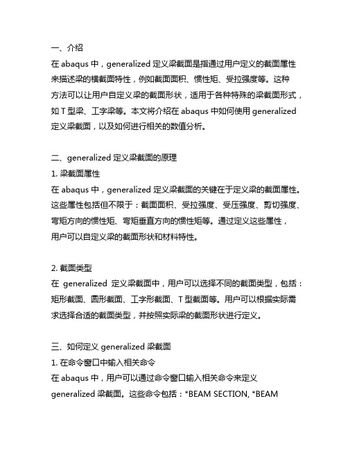
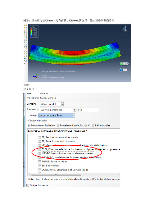
例子:梁长度为1500mm,均布荷载150N/mm,简支梁,输出梁中间截面弯矩
步骤:
定义输出
网格划分好之后,把需要输出弯矩的那个截面上所有的单元(element,就是一个个小方格)定义成一个SET方便以后选择:
Tools---set---Creat
再定义一个set,这个set包括这个截面上所有节点
定义完之后,然后最后算完之后:
选择截面一侧的elements (事先定义好的set)
为了方便查看有没有选错,可以把上面的HIGHLIGHT勾上,图中就会高亮显示了,方便看有没有选错。
然后就会出现:
其中双箭头的是弯矩,单箭头是剪力(经手算,这个结果很正确!!!!)
然后上面那个是这个面的主弯矩(个方向弯矩合力),看每个方向的弯矩,可以这样:
然后就有各个方向的弯矩了
双箭头的就是弯矩,单箭头是各个方向剪力
然后找到最大的那个双箭头(弯矩)的数值,就是要求的了。
abaqus中generalized定义梁截面
一、介绍在abaqus中,generalized定义梁截面是指通过用户定义的截面属性来描述梁的横截面特性,例如截面面积、惯性矩、受拉强度等。
这种方法可以让用户自定义梁的截面形状,适用于各种特殊的梁截面形式,如T型梁、工字梁等。
本文将介绍在abaqus中如何使用generalized 定义梁截面,以及如何进行相关的数值分析。
二、generalized定义梁截面的原理1. 梁截面属性在abaqus中,generalized定义梁截面的关键在于定义梁的截面属性。
这些属性包括但不限于:截面面积、受拉强度、受压强度、剪切强度、弯矩方向的惯性矩、弯矩垂直方向的惯性矩等。
通过定义这些属性,用户可以自定义梁的截面形状和材料特性。
2. 截面类型在generalized定义梁截面中,用户可以选择不同的截面类型,包括:矩形截面、圆形截面、工字形截面、T型截面等。
用户可以根据实际需求选择合适的截面类型,并按照实际梁的截面形状进行定义。
三、如何定义generalized梁截面1. 在命令窗口中输入相关命令在abaqus中,用户可以通过命令窗口输入相关命令来定义generalized梁截面。
这些命令包括:*BEAM SECTION, *BEAMGENERAL SECTION等。
用户可以根据具体的梁截面形式选择合适的命令,并按照命令提示依次输入截面属性参数、材料参数等信息。
2. 使用abaqus CAE进行图形化定义除了通过命令窗口输入命令外,用户还可以使用abaqus CAE进行图形化界面的定义。
在abaqus CAE中,用户可以通过菜单栏中的梁截面定义工具进行相关操作。
通过图形化界面,用户可以方便地定义梁截面属性、截面类型等信息。
四、使用generalized梁截面进行数值分析1. 定义梁截面在进行数值分析前,用户需要先定义具体的梁截面属性。
通过上述介绍的方法,用户可以在abaqus中定义generalized梁截面,并将其与具体的梁单元相对应。
ABAQUS输出实体单元某一截面的弯矩
例子:梁长度为1500mm,均布荷载150N/mm,简支梁,输出梁中间截面弯矩
步骤:
定义输出
网格划分好之后,把需要输出弯矩的那个截面上所有的单元(element,就是一个个小方格)定义成一个SET方便以后选择:
Tools---set---Creat
再定义一个set,这个set包括这个截面上所有节点
定义完之后,然后最后算完之后:
选择截面一侧的elements (事先定义好的set)
为了方便查看有没有选错,可以把上面的HIGHLIGHT勾上,图中就会高亮显示了,方便看有没有选错。
然后就会出现:
其中双箭头的是弯矩,单箭头是剪力(经手算,这个结果很正确!!!!)
然后上面那个是这个面的主弯矩(个方向弯矩合力),看每个方向的弯矩,可以这样:
然后就有各个方向的弯矩了
双箭头的就是弯矩,单箭头是各个方向剪力
然后找到最大的那个双箭头(弯矩)的数值,就是要求的了。
ABAQUS计算矩形截面梁详解版
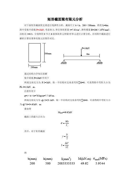
矩形截面梁有限元分析对下面矩形截面简支梁进行线弹性分析,截面尺寸b ×h :200×500mm ,跨度L=6m ,跨中受集中荷载F=10kN ,考虑体力,单位体积重量γ=7.85t/m ³,弹性模量E=206×103N/mm 2,泊松比ν=0.3,分别利用8节点6面体块单元和梁/杆单元进行计算分析,并对跨中截面进行解析计算结果和有限元结果作对比。
通过结构力学知识求解 集中荷载F=10kN 作用下两端支座反力为F/2=5kN ,取一半结构对支座求弯矩∑M=0,可求得跨中弯矩大小为FL/4=15kN .m 。
自重作用下q=γ×b ×h=785kg/m=7.7 kN/m 。
两端支座反力为qL/2=23.1kN ,取一半结构对支座求弯矩∑M=0,可求得跨中弯矩大小为qL 2/8=34.65kN .m 。
叠加得M max =49.62kN截面上的最大正应力zMyI σ=其中,对于矩形截面2h y =312bh I =得b(mm)h(mm)I(mm 4)M(kN.m)σmax (MPa)200500208333333349.62 5.9544200mm500mm3单位:建议采用国际单位制采用m、kg、N、s国际单位制时,重力加速度9.8m/s2,质量为kg,密度为7850 kg/m3,E=206×109Pa,泊松比ν=0.3,ABAQUS操作打开ABAQUS界面开始→所有程序→ABAQUS6.10-1→ABAQUS CAE,依次出现创建Part创建Part,重新命名liang23,选择三维(3D)可变形体(Deformable)实体(Solid)单元,建模方式选择拉伸(Extrusion),截面的大致尺寸(Approximate site)便于建模,默认即可。
continue继续点击,以坐标的格式创建模型。
依次在中输入(0,0)回车,(-3,0)回车,(-3,-0.5)回车,(0,-0.5)回车,(0,0)回车,点击下图中的或点击一次鼠标中键,继续点击下图中的或点击一次鼠标中键,(注:点击一次鼠标中键等价于)出现如下对话框Depth表示拉伸(Extrusion)距离,取值为0.1,继续,出现下图(此模型为1/4半梁,之所以不一次建好,是为了后续工作中跨中施加一个集中力)点击保存一下(注:ABAQUS不自动保存)文件名(File)取(liang23)继续回到Property(特性)二、进入Module(模块)列表中选择Property(特性)功能模块,出现如下点击,创建材料,出现Name随便命名比如默认的(Material-1),点击,选择下拉菜单Density(密度)取为7850,(注:统一成国际单位7.85t/m3=7850 kg/m3)继续点击(力学特性)选择下拉菜单Elasticity(弹性)→Elastic(弹性)出现在(杨氏模量,即弹性模量)写入206e9,(注:E=206×103N/mm2=206×109Pa),在(泊松比)写入0.3,(注:ν=0.3,)继续创建截面属性,点击,出现(可重命名,也可默认)继续出现继续。
Abaqus切削仿真常见问题及其解决个人总结
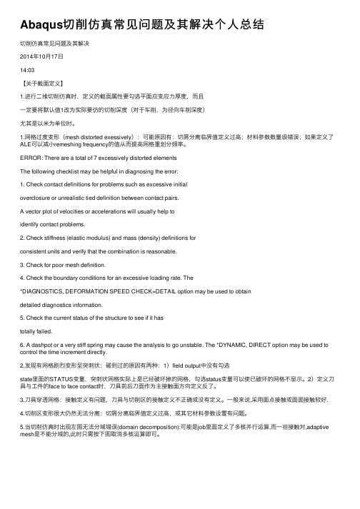
Abaqus切削仿真常见问题及其解决个⼈总结切削仿真常见问题及其解决2014年10⽉17⽇14:03【关于截⾯定义】1.进⾏⼆维切削仿真时,定义的截⾯属性要勾选平⾯应变应⼒厚度,⽽且⼀定要将默认值1改为实际要仿的切削深度(对于车削,为径向车削深度)尤其是以⽶为单位时。
1.⽹格过度变形(mesh distorted exessively):可能原因有:切屑分离临界值定义过⾼;材料参数数量级错误;如果定义了ALE可以减⼩remeshing frequency的值从⽽提⾼⽹格重划分频率。
ERROR: There are a total of 7 excessively distorted elementsThe following checklist may be helpful in diagnosing the error:1. Check contact definitions for problems such as excessive initialoverclosure or unrealistic tied definition between contact pairs.A vector plot of velocities or accelerations will usually help toidentify contact problems.2. Check stiffness (elastic modulus) and mass (density) definitions forconsistent units and verify that the combination is reasonable.3. Check for poor mesh definition.4. Check the boundary conditions for an excessive loading rate. The*DIAGNOSTICS, DEFORMATION SPEED CHECK=DETAIL option may be used to obtaindetailed diagnostics information.5. Check the current status of the structure to see if it hastotally failed.6. A dashpot or a very stiff spring may cause the analysis to go unstable. The *DYNAMIC, DIRECT option may be used to control the time increment directly.2.发现有⽹格剧烈变形呈突刺状:碰到过的原因有两种:1)field output中没有勾选state⾥⾯的STATUS变量,突刺状⽹格实际上是已经破坏掉的⽹格,勾选status变量可以使已破坏的⽹格不显⽰。
abaqus输出选项类型设定
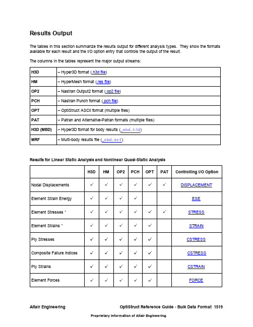
Altair Engineering OptiStruct Reference Guide - Bulk Data Format 1519Results OutputThe tables in this section summarize the results output for different analysis types. They show the formats available for each result and the I/O option entry that controls the output of the result. The columns in the tables represent the major output streams:H3D – Hyper3D format (.h3d file )HM – HyperMesh format (.res file )OP2– Nastran Output2 format (.op2 file)PCH– Nastran Punch format (.pch file)OPT– OptiStruct ASCII format (multiple files)PAT – Patran and Alternative-Patran formats (multiple files)H3D (MBD)– Hyper3D format for body results (_mbd.h3d)MRF– Multi-body results file (_mbd.mrf )Results for Linear Static Analysis and Nonlinear Quasi-Static AnalysisH3DHMOP2PCHOPTPATControlling I/O Option Nodal Displacements DISPLACEMENTElement Strain Energy ESE Element Stresses *STRESS Element Strains *STRAIN Ply StressesCSTRESS Composite Failure Indices CSTRESS Ply Strains CSTRAIN Element ForcesFORCEGrid Point Stresses GPSTRESSSPC Forces SPCFORCEMPC Forces MPCFORCEGrid Point Forces GPFORCEApplied Loads OLOADResults for Linear Steady-state Heat Transfer AnalysisH3D OP2PCH Controlling I/O OptionNodal Temperatures THERMALElement Fluxes and Gradients FLUXResults for Normal Modes AnalysisH3D HM OP2PCH OPT PAT Controlling I/O OptionEigenvectors DISPLACEMENTElement Kinetic Energy EKEElement Strain Energy ESEGrid Point Stress GPSTRESSElement Stresses *STRESSMPC Forces MPCFORCEAltair Engineering OptiStruct Reference Guide - Bulk Data Format 1521Nodal Pressures (Fluid)PRESSUREResults for Complex Eigenvalue AnalysisH3DOP2PCHControlling I/O Option EigenvectorsDISPLACEMENTResults for Linear Buckling AnalysisH3DHMOP2PCHOPTControlling I/O OptionEigenvectorsDISPLACEMENTResults for Frequency Response AnalysisH3D HMOP2PCH OPTControlling I/O Option Nodal DisplacementsDISPLACEMENT Modal Participation Displacements SDISPLACEMENTElement Energy Loss Per Cycle EDE Element Kinetic Energy EKE Element Strain Energy ESE Nodal VelocitiesVELOCITY Modal Participation Velocities SVELOCITY Nodal AccelerationsACCELERATIONModal Participation Accelerations SACCELERATIONElement Stresses *STRESSElement Strains *STRAINElement Forces FORCESPC Forces SPCFORCEMPC Forces MPCFORCEGrid Point Forces GPFORCEPower Flow Field POWERFLOWResults for Coupled Frequency Response Analysis of Fluid-structural Models (Acoustic Analysis)H3D OP2PCH Controlling I/O OptionNodal Displacements DISPLACEMENTModal Participation Displacements SDISPLACEMENTNodal Velocities VELOCITYModal Participation Velocities SVELOCITYNodal Accelerations ACCELERATIONModal Participation Accelerations SACCELERATIONNodal Pressures (Fluid)PRESSUREElement Stresses *STRESSAltair Engineering OptiStruct Reference Guide - Bulk Data Format 1523Element Strains *STRAIN Element ForcesFORCESPC Forces SPCFORCEMPC ForcesMPCFORCEGrid Point ForcesGPFORCEPower Flow FieldPOWERFLOWResults for Transient AnalysisH3DHMOP2PCHControlling I/O Option Nodal DisplacementsDISPLACEMENT Modal Participation Displacements SDISPLACEMENTNodal VelocitiesVELOCITY Modal Participation Velocities SVELOCITY Nodal AccelerationsACCELERATION Modal Participation Accelerations SACCELERATIONElement Stresses *STRESS Element Strains *STRAIN Element Forces FORCE MPC ForcesMPCFORCEResults for Random Response AnalysisOP2PCH Controlling I/O OptionDisplacement PSD X YPEAK, X YPLOT, X YPUNCHVelocity PSD X YPEAK, X YPLOT, X YPUNCHAcceleration PSD X YPEAK, X YPLOT, X YPUNCHPSD Element Stress STRESS, X YPEAK, X YPLOT, X YPUNCHPSD Element Strain STRAIN, X YPEAK, X YPLOT, X YPUNCHRMS Element Stress STRESS, X YPEAK, X YPLOT, X YPUNCHRMS Element Strain STRAIN, X YPEAK, X YPLOT, X YPUNCH Results for Multi-body Dynamics AnalysisH3D HM OP2H3D(MBD)MRF Controlling I/OOptionNodal Displacements DISPLACEMENTNodal Velocities VELOCITYNodal Accelerations ACCELERATIONElement Stresses *STRESSElement Strains *STRAINBody time historyAltair Engineering OptiStruct Reference Guide - Bulk Data Format 1525System time history Marker time historyREQUESTResults for Fatigue AnalysisH3DControlling I/O OptionElement Life LIFE Element DamageDAMAGEOptimization ResultsH3DHMOP2PCHOPTPATControlling I/O OptionElement Density DENSITY Element Thickness THICKNESS Ply Thickness THICKNESS % Thickness THICKNESS ShapeSHAPE*The element stress and strain results written to the various output streams are not always the same.Please refer to the following pages for more details on the stress results available in the different output streams:Strain Results Written in HyperView .h3d Format Strain Results Written in Nastran .op2 and .pch Formats Strain Results Written in HyperMesh .res Format Stress Results Written in HyperView .h3d Format Stress Results Written in Nastran .op2 and .pch Format Stress Results Written in HyperMesh .res FormatStrain Results Written in HyperView .h3d Format 1-D ElementsALL, DIRECT and TENSOR optionsCELAS StrainCROD Axial StrainCBAR Longitudinal Strain SACCBAR Longitudinal Strain SADCBAR Longitudinal Strain SAECBAR Longitudinal Strain SAFCBAR Longitudinal Strain SAMINCBAR Longitudinal Strain SAMAXCBAR Longitudinal Strain SBCCBAR Longitudinal Strain SBDCBAR Longitudinal Strain SBECBAR Longitudinal Strain SBFCBAR Longitudinal Strain SBMINCBAR Longitudinal Strain SBMAXCWELD Axial StrainCWELD Maximum Strain ACWELD Minimum Strain ACWELD Maximum Strain BCWELD Minimum Strain BCWELD Maximum Shear StrainVON and PRINC optionsVon Mises Strain2-D ElementsALL and TENSOR optionsResults are calculated by HyperView.DIRECT optionVon Mises StrainMaximum Principal StrainVon Mises Strain (Z1)Von Mises Strain (Z2)Von Mises Strain (mid)P1 (major) Strain (Z1)P1 (major) Strain (Z2)P1 (major) Strain (mid)P3 (minor) Strain (Z1)P3 (minor) Strain (Z2)P3 (minor) Strain (mid)Normal X Strain (Z1)Normal X Strain (Z2)Normal X Strain (mid)Normal Y Strain (Z1)Normal Y Strain (Z2)Normal Y Strain (mid)Shear XY Strain (Z1)Shear XY Strain (Z2)Shear XY Strain (mid)Principal Strain Angle (Z1)Principal Strain Angle (Z2)Principal Strain Angle (mid)VON optionVon Mises StrainPRINC optionVon Mises StrainMaximum Principal Strain3-D elementsALL and TENSOR optionsResults are calculated by HyperView.DIRECT optionVon Mises StrainSigned Von Mises StrainP1 (major) Strain (solid)P2 (mid) Strain (solid)P3 (minor) Strain (solid)Normal X Strain (solid)Normal Y Strain (solid)Normal Z Strain (solid)Shear XY Strain (solid)Shear YZ Strain (solid)Shear XZ Strain (solid)VON optionVon Mises StrainPRINC optionVon Mises StrainMaximum Principal StrainComments1.In the TENSOR mode, we pass tensor components to HyperView which then calculates derived resultson-the-fly.2.For frequency response loadcases, only the TENSOR mode is available.Altair Engineering OptiStruct Reference Guide - Bulk Data Format1527Strain Results Written in Nastran .op2 and .pch Formats Static, Eigenvalue, Transient and Multi-body Loadcases1-D elementsNone.2-D elementsFibre Distance (Z1)Normal XX Strain (Z1)Normal YY Strain (Z1)Shear XY Strain (Z1)Principal Strain Angle (Z1)Major Principal Strain (Z1)Minor Principal Strain (Z1)Von Mises Strain (Z1)Fibre Distance (Z2)Normal XX Strain (Z2)Normal YY Strain (Z2)Shear XY Strain (Z2)Principal Strain Angle (Z2)Major Principal Strain (Z2)Minor Principal Strain (Z2)Von Mises Strain (Z2)3-D elementsNormal XX StrainShear XY StrainMajor Principal StrainMajor Principal X CosineMid Principal X CosineMinor Principal X CosineMean StrainVon Mises StrainNormal YY StrainShear YZ StrainMid Principal StrainMajor Principal Y CosineMid Principal Y CosineMinor Principal Y CosineNormal ZZ StrainShear XZ StrainMinor principal StrainMajor Principal Y CosineMid Principal Y CosineMinor Principal Y CosineFrequency Response Loadcases1-D elementsNone.2-D elementsFibre Distance (Z1)Normal XX Strain (real) (Z1)Normal XX Strain (imag) (Z1)Normal YY Strain (real) (Z1)Normal YY Strain (imag) (Z1)Shear XY Strain (real) (Z1)Shear XY Strain (imag) (Z1)Fibre Distance (Z2)Normal XX Strain (real) (Z2)Normal XX Strain (imag) (Z2)Normal YY Strain (real) (Z2)Normal YY Strain (imag) (Z2)Shear XY Strain (real) (Z2)Shear XY Strain (imag) (Z2)3-D elementsNormal XX Strain (real)Normal YY Strain (real)Normal ZZ Strain (real)Shear XY Strain (real)Shear YZ Strain (real)Shear XZ Strain (real)Normal XX Strain (imag)Normal YY Strain (imag)Normal ZZ Strain (imag)Shear XY Strain (imag)Shear YZ Strain (imag)Shear XZ Strain (imag)Comments1.The order above reflects the contents of the OP2 file, but post-processors such as HyperView maydisplay results in a different manner.Altair Engineering OptiStruct Reference Guide - Bulk Data Format1529Strain Results Written in HyperMesh .res Format Static, Eigenvalue, Transient and Multi-body LoadcasesALL, DIRECT and TENSOR optionsVon Mises StrainMaximum Principal StrainVon Mises Strain (Z1)Von Mises Strain (Z2)Von Mises Strain (mid)P1 (major) Strain (Z1)P1 (major) Strain (Z2)P1 (major) Strain (mid)P1 (major) Strain (max)P3 (minor) Strain (Z1)P3 (minor) Strain (Z2)P3 (minor) Strain (mid)P3 (minor) Strain (min)Normal X Strain (Z1)Normal X Strain (Z2)Normal X Strain (mid)Normal Y Strain (Z1)Normal Y Strain (Z2)Normal Y Strain (mid)Shear XY Strain (Z1)Shear XY Strain (Z2)Shear XY Strain (mid)Principal Strain Angle (Z1)Principal Strain Angle (Z2)Principal Strain Angle (mid)Signed Von Mises Strain (solid)P1 (major) Strain (solid)P2 ( mid ) Strain (solid)P3 (minor) Strain (solid)Normal X Strain (solid)Normal Y Strain (solid)Normal Z Strain (solid)Shear XY Strain (solid)Shear YZ Strain (solid)Shear XZ Strain (solid)VON optionVon Mises StrainPRINC optionVon Mises StrainMaximum Principal StrainFrequency Response LoadcasesNormal X Strain (Z1) (comp)Normal X Strain (Z2) (comp)Normal Y Strain (Z1) (comp)Normal Y Strain (Z2) (comp)Shear XY Strain (Z1) (comp)Shear XY Strain (Z2) (comp)Normal X Strain (solid) (comp)Normal Y Strain (solid) (comp)Normal Z Strain (solid) (comp)Shear XY Strain (solid) (comp)Shear YZ Strain (solid) (comp)Shear XZ Strain (solid) (comp)Comments1."Von Mises Strain" and "Maximum Principal Strain" apply to 1-D, 2-D, and 3-D elements simultaneously.Other results apply to 2-D or 3-D elements exclusively. There are no specific results for 1-D elements.2.For frequency response loadcases, (comp) may be replaced by (real) (imag) (magn) and/or (phas),depending on the complex format request.3."Maximum Principal Strain" is the maximum absolute principal strain:max(abs(P1(Z1)),abs(P1(Z2)),abs(P3(Z1)),abs(P3(Z2))) for shells.max(abs(P1),abs(P2),abs(P3)) for solids.4."P1 (major) Strain (max)" is the maximum major principal strain:max(P1(Z1),P1(Z2)).5."P3 (minor) Strain (min)" is the minimum minor principal strain:min(P3(Z1),P3(Z2)).6."Signed Von Mises Strain" is the Von Mises strain with traction/compression sign:sign(P1+P2+P3) * VonMises.Altair Engineering OptiStruct Reference Guide - Bulk Data Format1531Stress Results Written in HyperView .h3d Format 1-D ElementsALL, DIRECT and TENSOR optionsCELAS StressCROD Axial StressCBAR Longitudinal Stress SACCBAR Longitudinal Stress SADCBAR Longitudinal Stress SAECBAR Longitudinal Stress SAFCBAR Longitudinal Stress SAMINCBAR Longitudinal Stress SAMAXCBAR Longitudinal Stress SBCCBAR Longitudinal Stress SBDCBAR Longitudinal Stress SBECBAR Longitudinal Stress SBFCBAR Longitudinal Stress SBMINCBAR Longitudinal Stress SBMAXCWELD Axial StressCWELD Maximum Stress ACWELD Minimum Stress ACWELD Maximum Stress BCWELD Minimum Stress BCWELD Maximum Shear StressCWELD Bearing StressVON and PRINC optionsVon Mises Stress2-D ElementsALL and TENSOR optionsResults are calculated by HyperView.DIRECT optionVon Mises StressMaximum Principal StressVon Mises Stress (Z1)Von Mises Stress (Z2)Von Mises Stress (mid)P1 (major) Stress (Z1)P1 (major) Stress (Z2)P1 (major) Stress (mid)P3 (minor) Stress (Z1)P3 (minor) Stress (Z2)P3 (minor) Stress (mid)Normal X Stress (Z1)Normal X Stress (Z2)Normal X Stress (mid)Normal Y Stress (Z1)Normal Y Stress (Z2)Normal Y Stress (mid)Shear XY Stress (Z1)Shear XY Stress (Z2)Shear XY Stress (mid)Principal Stress Angle (Z1)Principal Stress Angle (Z2)Principal Stress Angle (mid)VON optionVon Mises StressPRINC optionVon Mises StressMaximum Principal Stress3-D ElementsALL and TENSOR optionsResults are calculated by HyperView.DIRECT optionVon Mises StressSigned Von Mises StressP1 (major) Stress (solid)P2 (mid) Stress (solid)P3 (minor) Stress (solid)Normal X Stress (solid)Normal Y Stress (solid)Normal Z Stress (solid)Shear XY Stress (solid)Shear YZ Stress (solid)Shear XZ Stress (solid)VON optionVon Mises StressPRINC optionVon Mises StressMaximum Principal StressAltair Engineering OptiStruct Reference Guide - Bulk Data Format1533Comments1.In the TENSOR mode, we pass tensor components to HyperView which then calculates derived resultson-the-fly.2.For frequency response loadcases, only the TENSOR mode is available.Stress Results Written in Nastran .op2 and .pch FormatsStatic, Eigenvalue, Transient and Multi-body Loadcases1-D elementsNone.2-D elementsFibre Distance (Z1)Normal XX Stress (Z1)Normal YY Stress (Z1)Shear XY Stress (Z1)Principal Stress Angle (Z1)Major Principal Stress (Z1)Minor Principal Stress (Z1)Von Mises Stress (Z1)Fibre Distance (Z2)Normal XX Stress (Z2)Normal YY Stress (Z2)Shear XY Stress (Z2)Principal Stress Angle (Z2)Major Principal Stress (Z2)Minor Principal Stress (Z2)Von Mises Stress (Z2)3-D elementsNormal XX StressShear XY StressMajor Principal StressMajor Principal X CosineMid Principal X CosineMinor Principal X CosineMean StressVon Mises StressNormal YY StressShear YZ StressMid Principal StressMajor Principal Y CosineMid Principal Y CosineMinor Principal Y CosineNormal ZZ StressShear XZ StressMinor principal StressMajor Principal Y CosineMid Principal Y CosineMinor Principal Y CosineAltair Engineering OptiStruct Reference Guide - Bulk Data Format1535Frequency Response Loadcases1-D elementsNone.2-D elementsFibre Distance (Z1)Normal XX Stress (real) (Z1)Normal XX Stress (imag) (Z1)Normal YY Stress (real) (Z1)Normal YY Stress (imag) (Z1)Shear XY Stress (real) (Z1)Shear XY Stress (imag) (Z1)Fibre Distance (Z2)Normal XX Stress (real) (Z2)Normal XX Stress (imag) (Z2)Normal YY Stress (real) (Z2)Normal YY Stress (imag) (Z2)Shear XY Stress (real) (Z2)Shear XY Stress (imag) (Z2)3-D elementsNormal XX Stress (real)Normal YY Stress (real)Normal ZZ Stress (real)Shear XY Stress (real)Shear YZ Stress (real)Shear XZ Stress (real)Normal XX Stress (imag)Normal YY Stress (imag)Normal ZZ Stress (imag)Shear XY Stress (imag)Shear YZ Stress (imag)Shear XZ Stress (imag)Comments1.The order above reflects the contents of the OP2 file, but post-processors such as HyperView maydisplay results in a different manner.2.For 2-D elements, results are printed at the center of the element, followed by results at each grid whencorner stresses are requested.3.For 3-D elements, results are printed at the center of the element, followed by results at each grid whencorner stresses are requested. In the OP2 format, regardless of the corner stress request, results are printed at each grid by duplicating results at the center.Stress Results Written in HyperMesh .res FormatStatic, Eigenvalue, Transient and Multi-body LoadcasesALL, DIRECT and TENSOR optionsVon Mises StressMaximum Principal StressVon Mises Stress (Z1)Von Mises Stress (Z2)Von Mises Stress (mid)P1 (major) Stress (Z1)P1 (major) Stress (Z2)P1 (major) Stress (mid)P1 (major) Stress (max)P3 (minor) Stress (Z1)P3 (minor) Stress (Z2)P3 (minor) Stress (mid)P3 (minor) Stress (min)Normal X Stress (Z1)Normal X Stress (Z2)Normal X Stress (mid)Normal Y Stress (Z1)Normal Y Stress (Z2)Normal Y Stress (mid)Shear XY Stress (Z1)Shear XY Stress (Z2)Shear XY Stress (mid)Principal Stress Angle (Z1)Principal Stress Angle (Z2)Principal Stress Angle (mid)Signed Von Mises Stress (solid)P1 (major) Stress (solid)P2 ( mid ) Stress (solid)P3 (minor) Stress (solid)Normal X Stress (solid)Normal Y Stress (solid)Normal Z Stress (solid)Shear XY Stress (solid)Shear YZ Stress (solid)Shear XZ Stress (solid)VON optionVon Mises StressPRINC optionVon Mises StressMaximum Principal StressAltair Engineering OptiStruct Reference Guide - Bulk Data Format1537Frequency response loadcasesNormal X Stress (Z1) (comp)Normal X Stress (Z2) (comp)Normal Y Stress (Z1) (comp)Normal Y Stress (Z2) (comp)Shear XY Stress (Z1) (comp)Shear XY Stress (Z2) (comp)Normal X Stress (solid) (comp)Normal Y Stress (solid) (comp)Normal Z Stress (solid) (comp)Shear XY Stress (solid) (comp)Shear YZ Stress (solid) (comp)Shear XZ Stress (solid) (comp)Comments1."Von Mises Stress" and "Maximum Principal Stress" apply to 1-D, 2-D, and 3-D elementssimultaneously. Other results apply to 2-D or 3-D elements exclusively. There are no specific results for 1-D elements.2.For frequency response loadcases, (comp) may be replaced by (real) (imag) (magn) and/or (phas),depending on the complex format request.3."Maximum Principal Stress" is the maximum absolute principal stress :max(abs(P1(Z1)),abs(P1(Z2)),abs(P3(Z1)),abs(P3(Z2))) for shells.max(abs(P1),abs(P2),abs(P3)) for solids.4."P1 (major) Stress (max)" is the maximum major principal stress :max(P1(Z1),P1(Z2)).5."P3 (minor) Stress (min)" is the minimum minor principal stress :min(P3(Z1),P3(Z2)).6."Signed Von Mises Stress" is the Von Mises stress with traction/compression sign:sign(P1+P2+P3) * VonMises.。
abaqus定义i型梁截面

abaqus定义i型梁截面
在Abaqus中定义I型梁截面可以通过以下步骤实现:
1. 创建截面,首先,在Abaqus中打开您的模型,然后转到
“模型”菜单并选择“创建”>“截面”>“梁截面”。
2. 选择类型,在弹出的对话框中,选择“梁截面”类型,并点
击“继续”。
3. 输入截面参数,在“梁截面”对话框中,选择“T型”或
“I型”作为您要定义的梁截面类型。
然后,根据您的设计要求输
入相关的截面尺寸,如上翼宽度、下翼宽度、翼厚度、腹板厚度等。
4. 添加材料属性,在定义完截面尺寸后,您需要为该截面指定
材料属性。
在“梁截面”对话框中,选择“材料”选项卡,然后为
该截面指定材料的弹性模量、泊松比等材料属性。
5. 完成定义,完成上述步骤后,点击“确定”以完成I型梁截
面的定义。
通过以上步骤,您就可以在Abaqus中成功定义I型梁截面。
在实际操作中,根据具体的工程需求和材料特性,您可能需要进一步调整截面参数和材料属性,以确保模型的准确性和可靠性。
希望这些步骤能帮助您成功定义I型梁截面。
ABAQUS实体单元内力输出
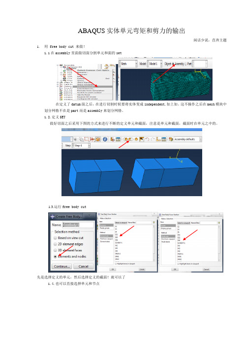
ABAQUS实体单元弯矩和剪力的输出闲话少说,直奔主题1.用 free body cut 来做!1.1在assembly里面做切面分割单元和面的set在定义了datum面之后,在进行切割时候要将实体变成independent,如上如。
这不操作之后在mesh模块中划分网格不在是part而是assembly来划分网格。
1.2.定义SET做好切面之后采用下图的方式来进行不断的定义单元和截面,注意是单元和截面,截面时在单元之中的。
1.3.运行free body cut先是选择定义的单元,然后选择定义的截面!就可以了1.4.也可以直接选择单元和节点首先选择的是节点所依附的单元然后是选择节点点击 ok输出的是有弯矩和没有弯矩时候的分量结果。
可以多定义截个这样的free body cut 然后输出注意:该种方法可以看任何单元的节点的内力值,不一定是一个截面上的!2.采用view cut来做(简单)3.Free body cut和view cut共同来做上述的图加上截面的选取进行定义截面注意:view cut的剪力正确,弯矩有偏差。
Free body cut相反。
但是划分的单元越小,距离真实值就越近!free body cut 中的 view cut来进行输出弯矩,轴力和剪力1. 打开 free body cut 创建方式为based on view cut2.找到了一个view cut ———allow for multiple cuts———copy3.结果显示如下:4.report———free body cut5,打开文件(上面的名字是可以修改的在view cut session 中)6.如果在显示中要打开moment,可以free body cut manager设置(素材和资料部分来自网络,供参考。
可复制、编制,期待您的好评与关注)。
- 1、下载文档前请自行甄别文档内容的完整性,平台不提供额外的编辑、内容补充、找答案等附加服务。
- 2、"仅部分预览"的文档,不可在线预览部分如存在完整性等问题,可反馈申请退款(可完整预览的文档不适用该条件!)。
- 3、如文档侵犯您的权益,请联系客服反馈,我们会尽快为您处理(人工客服工作时间:9:00-18:30)。
Defining the surface sectionSection output requests are available only for sections defined using element-based surfaces (see“Element-based surface definition,” Section 2.3.2). Consequently, the sections must be defined using faces of continuum elements although other types of elements (beams, membranes, shells, springs, dashpots, etc.) can be attached to the section.Calculation of accumulated quantities on the section (such as the total force) involves nodal quantities associated with elements on one side of the section only. Therefore, the surface definition should use elements only from one side of the section (the “base elements,” as defined in “Prescribed assembly loads,” Section 32.5.1), thus precisely identifying the side from which accumulated quantities are computed.Since the section usually cuts through the mesh in a typical section output request, automatic generation of the surface cannot be used. Specifying the element faces gives exact control over which element faces formthe surface, which is essential when defining a cross-section through a solid body.You must specify the name of the surface for which output is being requested.Surfaces that are defined in a restart analysis can be used only for section output requests. The newly defined surface cannot be used for any other purpose (such as a contact pair or pre-tension section definition).Use either of the following options: Input FileUsage:*SECTION PRINT, NAME=section_name,SURFACE=surface_name*SECTION FILE, NAME=section_name,SURFACE=surface_nameSelecting the coordinate system in which output is desiredYou can specify the choice of coordinate system in which the section output is desired. By default, thecomponents of vector quantities associated with the section are obtained with respect to the global system of coordinates. Alternatively, you can specify that output is desired in a local system as defined below. Input FileUse either of the following options: Usage:*SECTION PRINT, NAME=section_name,SURFACE=surface_name,AXES=GLOBAL or LOCAL*SECTION FILE, NAME=section_name,SURFACE=surface_name,AXES=GLOBAL or LOCALDefining a coordinate system local to the surface sectionYou can allow Abaqus/Standard to define the local system, or you can specify it directly.Default local systemThe default local system is particularly useful when the section is flat or almost flat. Though it can also be used in the case when the defined surface is curved, the default local system may be irrelevant for such problems.The default system is defined by a straight line in two-dimensional and axisymmetric cases or by a plane in three-dimensional cases, fitted (in a least square sense) through the nodes belonging to the section. The anchor point (origin) of the local system is the centroid of the projection of the surface on the fitted line or plane. The local directions are given by the normal (1-direction) and the tangent direction (the 2-direction in two-dimensional and axisymmetric cases) or the tangent directions (the 2- and 3-directions in three-dimensional cases) to the fitted line or plane. When several straight lines or planes can be fit equally well between the nodes defining the section (for example, a closed circular or spherical surface), the original local directions will be parallel to the global axes.The positive local 1-direction is selected such that it will form an acute angle with the average normal direction to the section, computed by averaging the positive normals to the element faces defining the section. If the average normal direction is zero (a closed surface), the 1-direction will form an acute angle with the global x-axis. If in two-dimensional or axisymmetric cases the 1-direction is within 0.1° of being normal to the global x-axis, it will form an acute angle with the global y-axis. In three-dimensional cases if the 1-direction is within 0.1° of being normal to the global X–Y plane, it will form an acute angle with the global z-axis.In two-dimensional and axisymmetric cases the local 2-direction is obtained by rotating the local1-direction counterclockwise by 90° about the anchor point. For three-dimensional situations the tangent directions of the surface are defined using the Abaqus conventions for local directions on surfaces in space (see “Conventions,” Section 1.2.2).Input File U se either of the following options to useUsage: the default local coordinate system:*SECTION PRINT, NAME=section_name,SURFACE=surface_name, AXES=LOCAL*SECTION FILE, NAME=section_name,SURFACE=surface_name, AXES=LOCALUser-specified local systemA user-specified local system is defined by specifying the origin and the directions of the axes. You can specify the origin (anchor point) by giving a node number or by specifying the coordinates of the anchor point.In two-dimensional and axisymmetric cases the local 2-direction is defined by specifying either a predefined node number or the coordinates of a point (point a) on the local 2-direction. The local1-direction is then obtained by rotating the local 2-axis clockwise by 90° about the anchor point (see Figure 4.1.2–1). If node numbers are used to definethe anchor point or the local directions, they must be connected to the mesh.Figure 4.1.2–1 User-defined local coordinate system.In three-dimensional cases either two predefined nodes or the coordinates of two points can be used to specify the local directions. A rectangular Cartesian coordinate system is then defined by its origin (the anchor point) and these two points. The first point (point a) must lie on the local 2-direction, and the second (point b) must be in the local 2–3 plane on the side of the local 3-direction. Although it is not necessary, it is intuitive to select the second pointsuch that it is on or near the local 3-direction (see Figure 4.1.2–1).If you do not specify the anchor point of the local system, it is taken to be the centroid of the projection of the surface on the fitted line or plane. If you do not specify the directions of the axes, the local system will be anchored at the specified anchor point and its axes will be parallel to the default axes of the projected surface. If neither the anchor point nor the directions are defined, the default local system will be used.In large-deformation analyses the surface section may rotate significantly during the deformation. By default, when output is requested in a local coordinate system, the system rotates with the average rigid body motion of the elements used to define the surface section (i.e., the local system and the output are updated during the analysis). The anchor point and local directions must then be specified relative to the undeformed configuration. You can choose to obtain vector output in the original local coordinate systeminstead. This choice is irrelevant in steps in which geometric nonlinearities are not considered.Input File Usage: Use either of the following options to specify the local coordinate systemdirectly:*SECTION PRINT , NAME=section_name ,SURFACE=surface_name ,AXES=LOCAL, UPDATE=YES or NOanchor point definitionaxes definition *SECTION FILE , NAME=section_name ,SURFACE=surface_name ,AXES=LOCAL, UPDATE=YES or NOanchor point definitionaxes definitionControlling the frequency of outputYou can control the frequency of section output by specifying the output frequency in increments. Unless a frequency of zero is specified to suppress output, the variables will always be output at the last increment of the step.Input FileUsage: Use either of the following options:*SECTION PRINT, NAME=section_name,SURFACE=surface_name, FREQUENCY=n*SECTION FILE, NAME=section_name,SURFACE=surface_name, FREQUENCY=nData file formatPrinted output is arranged in tables. The first line of the table contains the name of the requested output variable (see “Abaqus/Standard output variable identifiers,” Section 4.2.1), and the second line contains the corresponding value. If a section output request is defined without any specified outputvariables, all appropriate variables associated with the current analysis type are outputs.If several section output requests to the data file are encountered in one particular step, separate tables will be created for each request. Each table has a header denoting the name of the section and the name of the surface used. In addition, if the output is requested in a local coordinate system, the global coordinates of the anchor point(会给出local coordinates 的原点在global coordinate 中的坐标) and the cosine directions of the local axes are output.Results file formatSeveral section output records (record numbers1580–1591 in “Results file output format,” Section 5.1.2) are output for each section output request to the results file. The actual collection of records to be written to the results file depends on the number of valid output requests. If a section output requestis defined without any specified output variables, all records relevant to the current analysis type are stored in the results file.Vector output in the sectionVector output associated with section output requests consists of the total force (SOF), the total moment (SOM), and the center of forces (SOCF这是表示一个点). Output variable SOF is computed as a vector sum of the stress-based (internal) nodal forces of the nodes in the surface.Output variable SOM is computed with respect to the origin of the coordinate system considered.Thus, if the output is requested in the global coordinate system, the total moment is computed about the global origin; if the output is requested in a local coordinate system, the moment is computed about the current anchor point of the local system. The coordinates of the current anchor point may change during the analysis if the localcoordinate system is updated. Output variables SOF and SOM are both reported in the coordinate system considered.The center of forces SOCF is computed as the closest point to the centroid of the section through which the total force SOF acts. SOCF is always reported in the global coordinate system. If the total force vector is equal to zero, the centroid of the section is reported as the center of forces SOCF.The total moment vector, SOM, will not necessarily equal the cross product of the center of force vector, SOCF, and total force vector, SOF. Forces acting on two different points of the section may have components acting in opposite directions, such that these force components generate a net moment but not a net force; therefore,the total moment may not arise entirely from the resultant force.Scalar output in the sectionScalar output associated with a section output request consists of the area of the defined section (SOAREA), the total heat flux (SOH) in heat transfer analysis, the total current (SOE) in electrical analysis, the total mass flow (SOD) in mass diffusion analysis, and the total pore fluid volume flux (SOP) in couple pore fluid diffusion-stress analysis. These output variables are computed as the algebraic sum of the scalar internal nodal fluxes (work-conjugate to the associated primary solution variables) of the nodes in the surface. For example, in heat transfer analysis the total heat flux (SOH) is the sum of the NFLUX values at the nodes on the surfaces.Limitations when using section output requests Section output requests are subject to the following limitations:Section output requests are available only for sections defined by an element-based surface. Thus, they can be used only for sections along faces ofcontinuum elements.∙When defining the section, elements on only one side of the section must be used. Abaqus/Standard identifies all elements attached to the surface on this side and computes the section outputvariables as in a free-body diagram.∙ form a closed surface, or be on the exterior of the body. Figure 4.1.2–2 presents some typical cases of valid surfaces. If the section cuts only partially through the mesh, a valid free-body diagram cannot be isolated (see Figure 4.1.2–3) and incorrect answers may be computed.Abaqus/Standard will attempt to identify theinvalid cases and will issue error or warning messages.Figure 4.1.2–2 Valid section definitions.Figure 4.1.2–3 Invalid section definitions.∙Elements attached to the section can be on either side of the surface but must not cross the defined section. Figure 4.1.2–3 presents a few invalid cases. In most cases Abaqus/Standard willsuccessfully identify elements that cross the surface, and warning messages will be issued. The elements will then not be considered in thecalculation of the section variables.∙For section output purposes, Abaqus/Standard will ignore the elements attached to the section for which it cannot establish whether they belong to one side or the other of the section (e.g., SPRING1 elements).∙Section output requests cannot be specified withina substructure.∙Section output requests cannot be specified in random response analyses.∙The total force and the total moment in the section are computed based only on the stresses (internal forces) in the identified elements. Thus,inaccurate results may be obtained if distributed body loads are present in these elements since their effect on the total force in the section is not included. Common examples are the inertial loading in dynamic analyses, gravity loads,distributed body forces, and centrifugal loads. In these cases the total force in the section may depend on the choice of elements used to define the section as illustrated in Figure 4.1.2–4(a).Assuming that gravity loading is the only active load, the element stresses will be different in the two elements. Hence, if the same section is defined first using element 1 and then using element 2, different answers for the total force will be obtained. In a similar way the effects of anydistributed body fluxes (heat, electrical, etc.) prescribed in the identified elements are not included.Figure 4.1.2–4 Total force in the section.Depending on which side of the surface is used to define the section, different answers will be obtained in analyses similar to the caseillustrated in Figure 4.1.2–4(b). Assuming a static analysis with the concentrated loads shown in the figure being the only active loads, a zero total force is reported if the section is defined using element 1 and a nonzero force equal to the sum of the concentrated loads is obtained if the section is defined using element 2.。