Landmarking and Feature Localization in Spine X-rays
基于深度学习的遥感影像耕地地块边界提取应用
马海荣.基于深度学习的遥感影像耕地地块边界提取应用[J ].中南农业科技,2023,44(12):129-133.农业信息实时、精准地获取是实现农业现代化发展的基础和关键,耕地信息是最重要的基础农业信息,地块又是组成耕地和农户生产经营的最小单位,对地块边界提取是精准农业实践的基础和前提,是实现耕地监测、作物种植监测、产量预测、农业风险评估等应用的重要基础数据[1-3]。
中国土地资源总量多,但人均耕地数量少,高质量的耕地少,可开发的后备资源少,耕地的数量和质量与中国粮食安全息息相关[4-6]。
随着社会经济的发展和城镇化进程的加剧,耕地面积在逐渐减少,从地块级别进行耕地监测有利于加强耕地保护和保证中国粮食安全。
因此,准确、快速地进行大范围内耕地地块信息提取具有重要意义。
遥感技术具有覆盖范围广、空间分辨率高、获取手段方便等特点,已成为获取耕地面积、作物分布、作物生长状况等农业信息的有效途径[7]。
但是耕地地块作为农业生产的基本单元,特别是在中国以小农为生产主体的生产方式下,大多面积小、分布零散、情况复杂、作物种植类型多样,使得在遥感影像上不同地块的光谱、纹理等遥感特征类内差异大,类间差别不明显,难以实现耕地地块边界准确高效地提取。
最开始基于遥感技术的耕地信息提取采用人机交互目视解译的方法实现,该方法也是应用最为广泛的方法,这种作业方式的耕地提取结果精准度依赖于解译者专业水平,并且人力物力成本高,可重复性差。
后来出现的基于像素纹理分析[8]、面向对象[9]、浅层机器学习[10,11](如随机森林、支持向量机、神经网络等)等方法采用浅层特征提取结构,需要人工进行参数选择和特征选取,无法自主提取分类特征,不能准确提取各种类型耕地,影响了提取结果的精度和准确性。
被广泛应用的深度学习方法可以通过训练大量样本数据,自主学习提取主要特征,无需人工参与且对复杂多变的情况具有更好的鲁棒性,在计算机视觉等领域取得了很好的效果,并被应用于耕地地块信息提取[12]。
基于改进水平集和区域生长的轮廓提取方法
Ap l a in Re e r h o mp tr p i t s a c fCo u e s c o
V0 _ 9 No 7 l2 . J1 0 2 u .2 1
基 于 改进 水 平 集 和 区域 生长 的轮 廓 提 取 方 法 木
S h a nvrt,C eg u6 0 4 , hn ) c i u nU i sy hn d 10 1 C ia ei
Ab t a t T i p p rp o o e e e e s t a e n t re r y d f rn e e e r h t eh ma r i ip e mp l l e s r c : h s a e r p s d a n w l v l e s d o ag t a i e e c st r s a c u n b an h p o a a i b g f o h sc s q e c s I ov d t e b u d r ty n tt e b c g o n S e t me g a in n ta i o a t o s I r e O a od t e e u n e . ts l e h o n ay sa i g a h a k r u d’ xr e r de ti r d t n lme h d . n o d rt v i h i b i d e si e i n g o i g, u r a d t e p o e s d i g Ssa d r e it n a et r s od T e t e ev d t eh p ln n s n r g o r w n i p t o w r h r c s e t f ma e’ t n ad d vai st h e h l . h n i r c ie i ・ o h h p c mp s Sc n o r By t e r t a n lssa d e p r n e i c t n,t i to a e v o - r e at r m a g t o a u ’ o tu . h o e i la ay i n x e i c me t rf a i v i o h smeh d c n r mo e n n t g tp rsfo tr e a
地理英语词汇
中文
地理因子 地理过程 地理分布 地理界线 地理综合 地理考察 综合考察 区域分析 区域分异 生存空间 生存承载能力 环境决定论 灾变论 地球 地球表面
英文
geographical factors geographical process geographical distribution geographical boundary geographical synthesis geographical survey integrated survey regional analysis regional differentiation living space life-carrying capacity environmental determinism catastrophe theory earth earth surface
中文
山 山脉 岭 峰 山麓 半岛 岛屿 群岛 海峡 地峡 海拔(高度) 相对高度 山嘴 盆地 山间盆地
英文
mountain mountain range, mountain chain range, ridge peak, mount piedmont peninsula island archipelago strait isthmus altitude, height above sea level relative height mountain spur basin intermountain basin
地球表层 地理系统 地理圈 景观圈 岩石圈 水圈 大气圈 土壤圈 生物圈 地圈 智能圈 技术圈 北半球 南半球 地球体
中文
英文
epigeosphere geosystem geographical sphere landscape sphere lithosphere hydrosphere atmosphere pedosphere biosphere geosphere noonsphere technosphere northern hemisphere southern hemisphere geoid
slam算法工程师招聘笔试题与参考答案(某世界500强集团)2024年
2024年招聘slam算法工程师笔试题与参考答案(某世界500强集团)(答案在后面)一、单项选择题(本大题有10小题,每小题2分,共20分)1、以下哪个不属于SLAM(Simultaneous Localization and Mapping)算法的基本问题?A、定位B、建图C、导航D、路径规划2、在视觉SLAM中,常用的特征点检测算法不包括以下哪一项?A、SIFT(Scale-Invariant Feature Transform)B、SURF(Speeded Up Robust Features)C、ORB(Oriented FAST and Rotated BRIEF)D、BOW(Bag-of-Words)3、SLAM(同步定位与映射)系统中的“闭环检测”功能主要目的是什么?A. 提高地图的精度B. 减少计算量C. 优化路径规划D. 增强系统稳定性4、在视觉SLAM中,以下哪种方法通常用于提取特征点?A. SIFT(尺度不变特征变换)B. SURF(加速稳健特征)C. ORB(Oriented FAST and Rotated BRIEF)D. 以上都是5、SLAM(Simultaneous Localization and Mapping)算法的核心目标是什么?A. 实现无人驾驶车辆在未知环境中的自主导航B. 构建三维空间地图并实时更新C. 实现机器人路径规划D. 以上都是6、以下哪种传感器不适合用于SLAM系统?A. 激光雷达B. 摄像头C. 声呐D. 超声波传感器7、以下关于SLAM(同步定位与映射)系统的描述中,哪个是错误的?A. SLAM系统通常需要在未知环境中进行定位与建图。
B. SLAM系统通常需要使用传感器来获取环境信息。
C. SLAM系统可以实时生成地图并更新位置信息。
D. SLAM系统不需要进行初始化定位。
8、以下关于视觉SLAM(视觉同步定位与映射)系统的描述中,哪个是正确的?A. 视觉SLAM系统只依赖于视觉传感器进行定位与建图。
跨领域迁移学习在自然语言生成任务中的应用研究

跨领域迁移学习在自然语言生成任务中的应用研究自然语言生成(Natural Language Generation, NLG)是人工智能领域的一个重要研究方向,它涉及将结构化数据转化为自然语言文本的过程。
随着大数据和深度学习技术的迅速发展,NLG在多个领域中得到了广泛应用,如机器翻译、文本摘要、对话系统等。
然而,在不同领域中进行NLG任务时,往往面临着数据稀缺和模型泛化能力不足等挑战。
为了解决这些问题,跨领域迁移学习被引入到NLG任务中,并取得了显著的研究进展。
一、跨领域迁移学习概述跨领域迁移学习是指将一个或多个源领域中学到的知识应用到目标领域中的过程。
在NLG任务中,源领域可以是一个或多个相关但不完全相同的任务,在这些任务上训练得到模型可以被应用于目标领域。
跨领域迁移学习可以通过共享模型参数、共享特征表示或共享训练数据等方式实现。
二、跨领域迁移学习的应用场景1. 机器翻译机器翻译是将一种自然语言文本转化为另一种自然语言文本的过程。
在跨领域迁移学习中,可以利用在一个或多个源领域上训练得到的翻译模型,将其应用于目标领域。
例如,在医学领域中,由于医学文本数据较少,可以利用通用领域的机器翻译模型进行迁移学习,以提高医学文本的翻译质量。
2. 文本摘要文本摘要是将一篇较长的文本转化为简洁、凝练的摘要的过程。
在跨领域迁移学习中,可以利用在一个或多个源领域上训练得到的摘要模型,将其应用于目标领域。
例如,在新闻报道中,由于每个新闻报道都有不同的主题和风格特点,在一个主题上训练得到的摘要模型可以通过跨领域迁移学习应用到其他主题上。
3. 对话系统对话系统是指与用户进行自然语言交互的系统。
在跨领域迁移学习中,可以利用在一个或多个源领域上训练得到的对话模型,将其应用于目标领域。
例如,在客服领域中,可以利用在其他行业的对话系统上训练得到的模型进行迁移学习,以提高客服对话系统的性能。
三、跨领域迁移学习方法1. 参数共享参数共享是指在源领域和目标领域之间共享模型参数的方法。
物体级语义视觉SLAM研究综述

第40卷第12期2023年12月控制理论与应用Control Theory&ApplicationsV ol.40No.12Dec.2023物体级语义视觉SLAM研究综述田瑞,张云洲†,杨凌昊,曹振中(东北大学信息科学与工程学院,辽宁沈阳110819)摘要:视觉同时定位与地图构建(Visual simultaneous localization and mapping,VSLAM)是自主移动机器人、自动驾驶、增强现实(AR)等领域的关键技术.随着深度学习的发展,准确高效的图像语义信息在VSLAM领域得到了广泛的应用.与传统SLAM相比,语义VSLAM利用语义信息提升了定位精度和鲁棒性,并通过物体级重建提高了环境感知能力,成为当前VSLAM领域的研究热点.本文对近年来优秀的物体级语义SLAM工作进行了阐述归纳和对比梳理,总结了该领域的4个关键问题,包括物体表达形式、物体初始化方法、融合语义信息的数据关联算法和融合物体级语义信息的后端优化方法.同时,对代表性方法进行了优缺点分析.最后,在现有技术成果和研究基础上,对物体级语义VSLAM面临的挑战和未来研究方向进行了展望和分析.当前物体级语义SLAM仍面临着物体关联不准确、物体优化框架不完善等问题.如何有效使用和维护语义地图以应用于决策规划等任务,以及融合多源信息以丰富视觉感知是未来的研究热点.关键词:视觉SLAM;数据关联;语义分割;物体级地图引用格式:田瑞,张云洲,杨凌昊,等.物体级语义视觉SLAM研究综述.控制理论与应用,2023,40(12):2160–2171DOI:10.7641/CTA.2023.30338Survey of object-oriented semantic visual SLAMTIAN Rui,ZHANG Yun-zhou†,YANG Ling-hao,CAO Zhen-zhong(College of Information Science and Technology,Shenyang Liaoning110819,China) Abstract:Visual simultaneous localization and mapping(VSLAM)is a key technology for autonomous robots,au-tonomous navigation,and AR applications.With the development of deep learning,accurate and efficient semantic infor-mation has been widely used in pared with traditional SLAM,semantic SLAM leverages semantic informa-tion to improve the accuracy and robustness of localization,and enhances environmental perception ability by object-level reconstruction,which has became the trend in VSLAM research.In this survey,we provide an overview of semantic SLAM techniques with state-of-the-art object SLAM systems.Four key issues of semantic SLAM are summarized,including ob-ject representation,object initialization methods,data association methods,and back-end optimization methods integrating semantic objects.The advantages and disadvantages of the comparison methods are provided.Finally,we propose the future work and challenges of object-level SLAM technology.Currently,semantic SLAM still faces problems such as inaccurate object association and an unified optimization framework has not yet been proposed.How to effectively use and maintain semantic maps for the application of decision and planning tasks,as well as integrate multi-source information to enrich visual perception,will be future research hotspots.Key words:visual SLAM;data association;semantic information;Semantic mappingCitation:TIAN Rui,ZHANG Yunzhou,YANG Linghao,et.al.Survey of Object-oriented Semantic visual SLAM. Control Theory&Applications,2023,40(12):2160–21711引言视觉同时定位与建图(visual simultaneous locali-zation and mapping,VSLAM)技术通过相机实现自主定位与地图构建,相较于激光雷达,相机具有低成本、低功耗、强感知等特点,且二维图像的语义信息更容易通过深度学习技术获取.结合语义信息对环境中的物体进行建模,并利用物体的语义不变性约束提升VSLAM的定位精度和鲁棒性成为当前研究的热点.本文着重对物体级语义VSLAM的发展和关键技术进行讨论:首先,阐述了物体级语义信息在SLAM中的收稿日期:2023−05−19;录用日期:2023−11−21.†通信作者.E-mail:*********************;Tel.:+86139****1976.本文责任编委:胡德文.国家自然科学基金项目(61973066,61471110)资助.Supported by the National Natural Science Foundation of China(61973066,61471110).第12期田瑞等:物体级语义视觉SLAM 研究综述2161重要作用;其次,归纳了物体级语义SLAM 技术的4个关键的问题(模型表达、物体初始化、数据关联、后端优化);最后,对语义SLAM 面临的挑战和未来发展方向进行了展望.本文结构框图如图1所示.图1本文结构框图Fig.1Structure of the survey2物体级语义VSLAM 系统架构物体级语义VSLAM 一般采用多线程的算法架构,分为前端和后端.前端主要由跟踪线程和检测线程构成:跟踪线程负责图像特征提取,并通过帧间特征匹配和局部BA(bundle adjustment)优化求解相机位姿;检测线程使用深度网络对输入图像进行语义信息提取,并将其送入到跟踪线程中.图像语义信息是基于当前帧的检测结果,因此,使用物体数据关联对不同帧的检测信息进行处理,并进行物体初始化.后端优化线程负责相机和物体位姿优化,以及对物体建模的参数进行调整.最终,系统构建了物体级的语义地图,实现环境的语义感知.语义信息的获取形式可以分为:目标检测[1–3]、语义分割[4–8]、实例分割[9–10].不同的语义信息获取方式会影响算法的实时性,通常,语义分割网络耗时更长,且语义分割得到的像素级分割结果存在信息冗余和误检,目标检测网络效率更高,但在复杂场景下容易出现漏检和误检的现象.后端优化方式可以分为独立优化和联合优化策略,例如,OA-SLAM(object assisted SLAM)[11]使用独立的线程来优化二次曲面参数,QuadricSLAM [12]则将物体和相机放在局部BA 的统一框架下优化.近年来,融合目标检测和实例分割的物体级SL-AM 成为研究的热点,该类方法通过多视图几何约束,利用物体检测框重建物体模型.重建模型可以分为二次曲面[13–20]、立方框[21]等.实例分割可以获得更准确的物体实例掩码,通常用于辅助物体特征提取和数据关联,实现更准确的目标跟踪[22].常见的物体级VSLAM 结构如图2所示.3物体级语义VSLAM 优势和应用传统的VSLAM 一般通过点、线、面等几何元素构建地图,例如,稀疏点云地图[23]、稠密点云地图[24]、网格地图[25–26]、TSDF(truncated signed distance field)地图[27]等.这些地图为自身定位和环境感知提供基础,使得VSLAM 技术得以广泛应用.随着应用场景的增加,人们发现传统VSLAM 方法在定位精度和算法鲁棒性上具有局限性,主要有如下原因:1)动态干扰,当前VSLAM 算法大多基于环境静态假设,特征匹配和优化容易受到外点干扰,导致跟踪精度变差或者丢失.2)光照变换,传统的视觉特征在光照变化或者暗光条件下,特征匹配和图像光度误差匹配失败,导致无法实现位姿估计,算法鲁棒性降低.3)高层次的语义感知需求,传统的VSLAM 在表征物体上具有局限性,不具有语义信息,无法满足人机交互等复杂任务的需求.深度学习技术的引入为VSLAM 定位和环境感知带了新的解决方法.基于深度学习的特征提取技术为VSLAM 在复杂光照条件下提供更稳定的匹配效2162控制理论与应用第40卷果[28–30],实例分割或目标检测为物体的运动属性判断提供可能,减少了VSLAM 在复杂环境中受动态干扰的影响[31–32].通过构建的物体级地图和模型表达,丰富了系统的环境感知能力[11,14–19].图2物体级语义VSLAM 结构图Fig.2Architecture of object VSLAM3.1利用物体信息提升定位精度当前,室内外场景下的VSLAM 算法已经得到了长足的发展,一些SLAM 算法能够准确地构建环境地图,并在一定程度上克服噪声、动态干扰和光照变化的影响.例如,ORB-SLAM [33]、RGBD-SLAM [34]、LS-D-SLAM [35]等.然而,在实际应用部署中,算法仍面临着场景动态干扰的影响.早期的解决方案中[23],使用运动一致性和基于外点剔除的RANSAC(random sample consensus)策略对由噪声干扰导致的错误特征匹配进行筛选,或者在优化中引入鲁棒核函数来降低动态特征的优化权重,例如,ORB-SLAM2[23]使用特征均匀提取和鲁棒核函数来降低错误匹配干扰.近年来,一些工作将物体检测结果的语义属性引入VSLAM 中,对场景中物体的动静态进行判断,并剔除动态物体的干扰[36–40].Detect-SLAM [41]通过目标检测剔除动态点,并通过特征匹配和扩展区域进行运动概率传播,在提升定位精度的同时提升了目标检测的稳定性.DS-SLAM [39]使用实例分割结果和运动一致性判断物体的运动属性,并将动态特征进行剔除以提升定位精度.Dyna-SLAM [40]将落在运动物体掩码内的特征作为外点剔除,从而提升其在动态场景下的定位鲁棒性.类似的,Kaveti 和Singh [42]提出了Light Field SLAM,通过合成孔径成像技术重建被遮挡的静态场景,不同于Bescos 等人[43]的算法,其进一步利用了重建背景的特征进行位姿跟踪以实现更好的定位性能.针对基于深度学习的动态物体检测通常存在漏检和错检问题,Ballester 等人[44]提出了DOT-SLAM,结合实例分割和多视图几何来生成动态物体掩码,并通过最小化光度误差进行跟踪.这种方法不仅提高了定位精度,还提高了语义分割的精度.上述工作的重点是通过剔除动态信息来提升自身定位的鲁棒和准确性,但忽略了对场景中移动物体状态的感知.作为VSLAM 对动态场景理解的扩展,结合运动跟踪的VSLAM 成为当前研究的热点.Wang 等人[45]首先提出了带有运动物体跟踪的SLAM,将自身位姿估计和动态物体位姿估计分解为两个独立的状态估计问题.Kundu 等人[46]结合SfM(structure from motion)和运动物体跟踪来解决运动场景下的SLAM 问题,该方法将系统输出统一到包含静态结构和运动物体轨迹的三维动态地图中.Huang 等人[47]提出了Cluster-VO,能够进行多个物体的运动估计.该方法提出了一种多层概率关联机制来高效地跟踪物体特征,利用异构条件随机场(conditional random filed,CRF)聚类方法进行物体关联,最后在滑动窗口内优化物体的运动轨迹.Bescos 等人[43]将运动物体与自身状态估计问题紧耦合到统一框架中,对跟踪点集使用主成分分析(principal component analysis,PCA)聚类和立方框建模,并使用动态路标点对自身位姿进行约束.第12期田瑞等:物体级语义视觉SLAM研究综述2163考虑到场景的先验约束,Twist SLAM[48]使用机械关节约束来限制物体在特定场景位姿估计的自由度,结合3D目标检测获得先验物体估计,使用语义信息来构建物体点簇地图,并利用静态簇(道路和房屋)来估计相机位姿.动态簇则通过速度的变化进行跟踪和约束.VDO-SLAM[49]使用聚类点的形式对物体进行状态估计,使用实例分割和稠密场景流,提高了动态物体观测的数量和关联质量,该方法将动态和静态结构集成到统一的估计框架中,实现了对相机位姿和物体位姿的联合估计.3.2利用物体信息提升定位鲁棒性传统的视觉定位大多采用手工描述了,如OR-B[50],SIFT[51]等特征,并使用基于视觉词袋(bag of words,BOW)进行定位,当图像视角变化或者光照发生明显改变时,该方案的视觉定位会失效.物体语义信息能有效克服大视角变换以及光照变换等情况,为VSLAM提供更鲁棒的定位.实时的物体级单目SLAM算法SLAM++[52]利用了一个大型物体数据库,使用单词袋来识别对象,实现鲁棒定位.Zins等[11]提出的OA-SLAM利用重建的物体级语义地图进行相机重定位.该方案结合了特征描述子和场景物体的重投影观测,利用物体的相对位置关系约束,在视角变化剧烈的场景下实现定位,提升了视觉定位的鲁棒性.Liu等[53]提出基于物体级描述符的定位方法.文献[54]提出基于深度网络的物体描述符定位方法.CubeSLAM[55]利用物体立方框和当前帧的目标检测约束,提升系统在无纹理场景下的定位鲁棒性. QuadricSLAM[12]提出基于二次曲面的物体观测约束,首次使用3D椭球作为路标,同时使用一个联合优化框架,将相机位姿和二次曲面联合优化.文献[56]利用单目视觉构建的物体级路标和物体先验大小约束,减少了单目定位的尺度漂移,提升了单目视觉的定位精度和鲁棒性.类似的方案如文献[57–58],采用物体先验尺度约束单目定位漂移.EAO-SLAM[21]则使用物体立方框约束构建观测误差,减少了定位漂移.可以看出,融合物体语义信息已经成为了提高视觉定位精度和鲁棒性的有效途径之一.语义信息已经广泛应用于SLAM系统的初始化、后端优化、重定位和闭环检测等阶段.因此,有效地处理和利用语义信息是提高定位精度的关键.3.3利用物体信息提升系统环境感知能力VSLAM构建的地图可以分为:稀疏点云地图[23]、稠密地图[27]、半稠密地图[24]、结构地图[59–60]、平面地图[61–65]、物体级地图[13–19,52]等.点云地图中仅具有点云结构信息,通常用于为SLAM提供定位约束.半稠密和稠密地图可以更精细地表达环境.结构地图和平面地图通过抽象的场景点线面的结构,为场景提供轻量级的地图表达.然而,上述的地图表达形式缺少对环境的高层次语义感知能力.近年来,随着自动驾驶、人机交互等领域的兴起,环境的语义感知越来越受到研究者的重视.语义信息的融入为SLAM的地图提供更为丰富的感知信息.早期的物体SLAM,例如,SLAM++[52]利用物体CAD模型构建语义地图,通过目标检测和识别,将先验物体数据库的物体加载在地图中.文献[37]将语义标签信息融合到稠密点云地图中,构建了稠密语义地图.CubeSLAM[55]和EAO-SLAM[21]通过立方框构建物体级地图.文献[13–19]构建了物体的二次曲面地图,同时估计了物体的大小、旋转和位置.相比于二次曲面和立方体的包络,超二次曲面可以通过调节二次模型参数适应不同形状的物体,丰富环境物体的表达.文献[66]使用超二次曲面构建室内场景的物体级地图.一些工作将抽象的语义标识加入到地图表达中,A VP-SL-AM[67]通过检测道路的车道线,交通标识等信息构建了轻量级的语义地图,用于实现准确的室外场景定位.另外,一些研究者将运动物体的感知信息加入到SLAM中,提出了SLAM-MOT[22,47,68],在构建场景稀疏点云地图的同时,表达物体的运动轨迹,构建包含运动信息的物体地图.例如,VDO-SLAM[49]提出利用语义信息构建环境结构,跟踪刚性物体的运动并估计其三维运动轨迹,其地图表示如图3所示.图3VDO-SLAM系统可视化地图[49],包含运动物体跟踪和三维轨迹Fig.3Visualization of Object tracking and trajectory estima tion of VDO-SLAM[49]可以看出,融合语义信息后,VSLAM的地图表达形式更加丰富.构建的物体级地图包含场景的高层次2164控制理论与应用第40卷语义信息,而且通过动态跟踪和联合位姿估计,可以获得动态物体的速度和运动轨迹估计,使得VSLAM 可以实时估计环境物体的运动轨迹,具有更丰富的环境感知能力.4物体语义的表达形式和初始化方法物体表达形式是物体级语义SLAM 进行环境感知的重要环节,传统的SLAM 算法使用几何特征,例如点、线、面等元素构建环境地图.这些几何特征能为SLAM 提供定位约束,并在一定程度上表征场景的感知信息,但缺少语义信息.SIFT [51],SURF [50]和ORB [50]是最常用的特征.利用稀疏点表达环境的视觉SLAM 方法[23,33]已经在三维场景重建领域取得了巨大的成功.然而,这类地图由三维空间中稀疏分布的点集构成,缺乏对物体位姿和边界的准确描述.因此,稀疏点云地图不能应用于复杂的任务,如路径规划、避障等.近年来,得益于深度学习检测技术的发展,SLAM 的地图构建已经由传统的几何表征转为语义描述,特别是物体级的描述.在物体表达上,可以分为:先验模型、几何模型、深度学习表征等.这些物体表达提升了SLAM 的语义感知能力,不同物体的表达如图4所示[12,52,55,69–71].图4物体语义的表达形式Fig.4Object representation method of object VSLAM4.1先验模型表达先验模型表达使用预先建立的先验数据库,通过检测–匹配的方式加载物体.如图4(a)所示,先验模型表达的代表为SLAM++[52].文献[72]提出使用检测立方框与先验CAD 模型进行ICP 匹配,通过物体路标约束,实现缺乏纹理的地下停车场定位.文献[73]使用预先集成或预定义的模型来进行对象跟踪,该工作的目标是建立一个具有物体标识的环境地图,并使用预集成的对象模型辅助定位,其结合了两种不同的深度网络输出结果来联合物体检测和对象的姿态估计.4.2几何模型表达几何模型通过参数化的二次曲面或者立方框实现,如图4(b)–4(c)所示.Nicholson 等人[12]提出了Quadric-SLAM,首次将二次曲面作为路标引入到SLAM 中,详细推导了如何利用多帧不同视角的目标检测观测数据构建约束,求解物体的二次曲面参数.并提出二次曲面投影观测模型,使得二次曲面参与位姿优化成为可能.后续的大多数基于二次曲面的SLAM 方案都是基于这个思路的延续[74].Hosseinzadeh 等人[75]提出了Structure Aware SLAM,在二次曲面路标的基础上加入了平面约束,使得二次曲面的建模精度进一步提高.Ok 等人[14]使用室外物体前向运动假设,提出了一种利用目标检测框、图像纹理以及语义尺度先验估计二次曲面参数的方法,降低了二次曲面初始化的难度,然而,该方法只能对车辆进行建模.Liao 等人[76]引入对称性假设,提出了物体感知S-LAM,利用物体对称性补全物体点云,进而根据物体点云拟合二次曲面.Chen 等人[77]针对物体前向平移运动假设,提出了一种基于物体凸包和目标检测的二次曲面初始化方法,为二次曲面初始化提供了新的思路.为了解决二次曲面初始化对噪声敏感的问题,Ti-第12期田瑞等:物体级语义视觉SLAM研究综述2165an等人[19]提出了一种参数分离的二次曲面初始化方法,将旋转和平移估计解耦估计,提升了初始化对检测框噪声的鲁棒性.利用物体对称性可以实现快速二次曲面初始化,Liao等人[78]提出的SO-SLAM是一种新颖的单目物体级语义SLAM,该方法使用三种具有代表性的空间约束,包括比例比例约束、对称纹理约束和平面支撑约束实现单帧视角下的二次曲面初始化.立方框表达的代表作是CubeSLAM[55],将物体模型参数化为三维立方框.EAO-SLAM[21]使用立方框和椭球对室内物体进行空间描述.然而,相比于立方框,二次曲面具有完备的数学模型表达和射影几何描述,更易于通过二次曲面重投影约束融合到SLAM的后端优化框架中,因此受到研究者的青睐.另外,一些物体模型表达方案采用物体聚类点描述,Cluster-SLAM[69]及后续的ClusterVO[47]均使用物体聚类点簇进行物体位姿估计和表达,如图4(d)所示.4.3深度学习表征粗略的几何模型往往不能表示物体的精确体积,而稠密点云需要大量的内存占用来存储地图.最近一些工作使用基于深度学习的特征进行模型表达,结合学习表征的物体级路标实现室外定位[79].DSP-SLAM[70]使用DeepSDF(signed distance fun-ction)网络[80]提取物体特征,并通过网络参数和表面重建损失函数进行物体表面恢复,构建场景的物体地图,如图4(e)所示.SceneCode[81]和Node-SLAM[71]则使用了深度网络中间层特征来表征物体.利用这些深度提取的特征和表面渲染误差函数,可以恢复物体的几何形状,如图4(f)所示.以上可知,物体的初始化表征方法决定了物体SLAM的地图表达形式,深度学习需要高算力的计算设备,且系统的实时性无法保证,几何模型可以准确描述物体的大小、旋转和位置,能完整表达物体的占据信息,且地图占用小,已经成为当前研究的热点.5物体级语义信息的数据关联方法基于深度学习的语义提取方法大多关注于单帧检测,而VSLAM在定位和建图环节均需要考虑时间和空间上的数据关联.针对物体级语义SLAM,解决不同帧之间的语义观测关联问题,确定同一语义对象在连续帧的关联性,是后续实现多帧优化的前提条件.当前数据关联方法可以分为两类:基于概率关联的方法和基于分配算法的关联方法.5.1基于概率关联方法该方法将属于物体的观测约束建模为概率分布模型,根据模型分布关系来确定帧间物体关联.Beipeng Mu等人[82]使用实例分割掩码的中心深度表征物体观测,并利用Dirichlet分布对观测进行建模,通过DP m-eans算法和最大似然估计(maximum likelihood estim-ation,MLE)迭代结果确定物体的数据关联.Bowm-an等人[83]使用期望最大化(expectation-maximization, EM)算法对物体路标进行软关联,并将物体路标作为约束因子与几何观测进行融合.文献[84]使用概率数据关联的方式解决动态环境下的物体关联.Iqbal和Gans等人[85]分析了不同物体点云深度分布之间的区别,使用层次密度聚类算法和非参数检验方法对物体进行关联.5.2基于分配算法的关联方法基于分配算法的关联方法能利用多帧观测解决帧间漏检等问题,为系统提供稳定的物体关联结果.文献[86]使用物体词袋方法构建成本矩阵,通过分配算法实现关联.OA-SLAM[11]使用目标检测结果和物体路标重投影的交并比(intersection over union,IoU)构建成本矩阵,并使用KM(kuhn-munkres,KM)算法进行分配.然而,由于有限的观测视角以及观测帧数,上述方法对于动态场景下的物体数据关联表现并不理想.为了解决上述问题,一些工作采用检测跟踪算法(track-by-detection)实现物体数据关联.Bewley等人[87]使用卡尔曼滤波器对检测框进行状态预测和更新,通过计算预测和检测结果的2D IoU 来度量匹配相似度,并使用匈牙利算法求解指派问题.针对单源相似度的局限性,Deep SORT(deep simple online and realtime tracking)[88]融入了外观信息,使用重识别网络提取的特征,增强了匹配性能,同时,其在匹配策略上增加了级联匹配模块,根据轨迹相似性进行关联,降低了遮挡目标ID切换的频率.Hosseinzadeh 等人[89]采用检测框内特征点投影匹配数量作为度量,该方法能够在一定程度上克服跟踪时的遮挡问题.可以看到,当前数据关联方法主要通过融合多源特征构建成本矩阵,并通过分配算法求解实现.然而,数据关联结果依赖于语义提取模块精度,当检测精度降低时会对关联结果产生影响,进而影系统的定位精度和鲁棒性.稳定可靠的数据关联方法是提升系统表现的有效途径之一.6融合物体级语义信息的后端优化方法在物体完成初始化后,需要利用后续观测信息对地图中的重建物体进行优化,根据物体是否参与相机位姿优化,后端优化策略可以分为独立优化策略和联合优化策略.根据是否需要跟踪场景中的动态物体,联合优化策略的因子图也有不同的形式.后端优化策略示意图如图5所示.2166控制理论与应用第40卷图5融合物体信息的语义VSLAM后端优化方法Fig.5Back-end of object VSLAM with object observations6.1独立优化策略如图5(a)所示,独立优化策略下,物体的位姿和模型参数单独进行优化,物体模型利用跟踪线程中提供的相机初始位姿进行优化.OA-SLAM[11]使用连续帧的目标检测结果对椭球参数单独优化,并在后端优化中使用优化后的物体路标对相机位姿进行优化.CubeSLAM[55]使用采样得分初始化立方框,并独立估计相机位姿和立方框参数,从而确保相机位姿估计的准确性.独立优化关注于物体重建,在进行物体位姿优化调整时无法对相机定位结果进行修正,当相机定位失败时,系统无法实现准确的自身定位和语义地图构建,没有充分利用语义信息辅助定位.6.2联合优化策略1)联合因子图,该方案将物体参数和位姿估计放在统一因子图中进行优化,并根据是否需要对动态物体进行位姿估计分别采用不同的因子图.静态场景的联合优化因子图如图5(b)所示,该方法通常适用于静态场景或采用动态特征剔除策略的SLAM算法.QuadricSLAM[12]将二次曲面参数和相机位姿优化优化放在联合优化中,构建了室内场景的语义地图.Tian等[19]提出的方法将初始化椭球和关键帧位姿放在统一优化因子图中进行优化,提升了室外场景下的定位精度和二次曲面建图准确性.动态场景的因子图如图5(c)所示,引入了动态物体位姿估计和模型参数优化的误差因子.VDO-SL-AM[49]使用物体语义信息和基于场景光流的特征关联,实现刚性物体位姿估计,将动态和静态结构放在统一的后端优化框架中.后续研究如[14–15,17,20]也将物体位姿优化放在局部建图线程中以实现联合优化.近年来,融合二次曲面路标观测的VSLAM成为了研究的热点[12,19,75,78].2)滑动窗口优化策略.相比于静态场景,动态场景下的物体观测容易受到漏检、遮挡等因素的干扰,基于关键帧的关联方案不能为动态物体提供准确的数据关联信息.为了克服这些问题,一些基于滑窗的优化方式被提出[43,47–48].滑动窗口由固定帧数的观测队列组成,当新的帧观测加入队列时,位于时序最早的帧观测被移出,同时,其维护的状态也通过滑窗边缘化的方式进行求解,如图6所示.图6滑动窗口优化结构示意图Fig.6Sliding window based optimization method滑动窗口优化将物体位姿和相机位姿放在统一优化框架中,由于运动物体的特点,使用滑窗优化可以有效利用连续帧的特征信息.DynaSLAM2[43]将场景静态结构,相机位姿以及动态物体运动轨迹维护在一个紧耦合的局部BA进行优化,通过目标检测的二维检测框构建物体位姿约束,使用舒尔补加速稀疏矩阵边缘化求解,解决滑窗优化的计算效率问题.Cluster-VO[47]使用点聚类的方式,将物体点和背景点放在滑窗内进行优化.该方法使用时间和空间双通道的关键帧管理策略保证计算效率,同时对遮挡的运动物体进行预测和跟踪.可以看出,滑窗的方式具有快速响应、参数优化更准确的特点,适用于动态物体的跟踪和位姿估计.基于因子图的联合优化可以有效利用关键帧信息,对室内场景的物体优化更准确.7未来发展和展望利用语义信息,SLAM可以适应动态和复杂环境下的定位,并通过物体级语义地图提升系统的环境感知能力.其技术可以应用于无人驾驶、机器人导航、智慧城市等领域.未来,融合语义信息的高层次信息可以为增强现实(AR)和虚拟现实(VR)提供更丰富的。
LandMarK解释思路与技术2
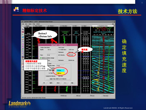
Button3 >Edit Data >Thickness Edit
由于采集方法不
同,两者间会存 在一定系统差异。 调整好填充速度
① ②
固定顶 部
后,只需微调即
可匹配好。大幅 度拉伸会造成层 速度畸变,是不
③
按下Apply后, 1916.95的位置将向 上微调至1893.8m
拉 伸 调 节
④
合理的。
Landmark ©2002. All Rights Reserved.
3
地震地质统层技术
Es3 Es4
技术方法
地质
Ek11
Ek12
Ek13
地震
Ek1顶构造图
层位精细标定、明确地质标志层地震响应特征的基础上,同时发挥测井精度高、地震覆盖 面广的优势,综合应用于地质统层,避免传统的地质、地震“背对背”的研究现状,保证 地质分层在地质标志层、沉积旋回、地震波阻特征上的一致性。 Landmark ©2002. All Rights Reserved.
Voxbody detect Shape cut
Values in range8/16-127 Voxbody as mask,convert to share Mem (Voxbody in share Mem)*1000=Fmax
Landmark ©2002. All Rights Reserved.
5
断层自动解释技术
技术方法
ESP
+
SeisWorks
+
EarthCube
Landmark ©2002. All Rights Reserved.
6
Faults Enhancement Workflow Summery
区域特征动态加权的IHS小波遥感图像融合
D0I l.9 9jsn1 0 -4 82 1.80 5 : 03 6 /i .0 03 2 .0 20 .6 .s
1 概 述
2 D gtl e h oo y P r , ce c d e h o o yP r f n h n Di r t f h n h n S e z e 0 7 C i a . i i c n lg ak S in ea c n lg a ko Na s a s i e z e , h n h n 5 5 , hn ) aT n T tc o S 1 8
wa e e e v ltr mot e sng i g uso t o t y mi i h i g o e i na li e t e I o b n st e a a t g so t e I r n f r a d e s n i ma e f i n me d wi d na c weg t fr g o lmu t— a h h n f ur . tc m i e dv a e f h HS ta s m h n o n wa e e r ns o o a h e e a b te u i n r s l,wh c o s f o n w u lc o o p n n s a t r ma c i g a d b i h ne s c v lt ta f r t c i v e t r f so e u t m i h c me r m e f l ol r c m o e t fe t h n n rg t s omp n n — o e tof mu ts e ta ma e a e HS ta s o ma i n.E pe i n a e u t n c t a h r po e t o s a p r n d n t g e e v to lip cr l i g f r I n f r to t r x rme t l r s ls i dia e t tt e p o s d me h d ha p a e t a va a e i r s r a i n of h n s e ta o a i n a d s a i l e a l n a e n a t e t o s p c l nf r t n p t t i e h nc me t h n o rme d . r i m o ad s t h h
- 1、下载文档前请自行甄别文档内容的完整性,平台不提供额外的编辑、内容补充、找答案等附加服务。
- 2、"仅部分预览"的文档,不可在线预览部分如存在完整性等问题,可反馈申请退款(可完整预览的文档不适用该条件!)。
- 3、如文档侵犯您的权益,请联系客服反馈,我们会尽快为您处理(人工客服工作时间:9:00-18:30)。
Landmarking and Feature Localization in Spine X-raysL. Rodney Long, National Library of Medicine, 8600 Rockville Pike, Bethesda, MD 20894/staff/long.phpGeorge R. Thoma, National Library of Medicine, 8600 Rockville Pike, Bethesda, MD 20894/staff/thoma.phpAbstractThe general problem of developing algorithms for the automated or computer-assisted indexing of images by structural contents is a significant research challenge. This is particularly so in the case of biomedical images, where the structures of interest are commonly irregular, overlapping, and partially occluded. Examples are the images created by digitizing film x-rays of the human cervical and lumbar spines. We have begun work toward the indexing of 17,000 such spine images for features of interest in the osteoarthritis and vertebral morphometry research communities. This work requires the segmentation of the images into vertebral structures with sufficient accuracy to distinguish pathology on the basis of shape, labeling of the segmented structures by proper anatomical name, and classification of the segmented, labeled structures into groups corresponding to high level semantic features of interest, using training data provided by biomedical experts. In this paper, we provide a technical characterization of the cervical spine images and the biomedical features of interest, describe the evolving technical approach for the segmentation and indexing problem, and provide results of algorithms to acquire basic landmark data and localization of spine regions in the images.KeywordsSegmentation, digitized x-ray, biomedical, classification, cervical spine, lumbar spine, ASM, image indexing, NLM, NIH, NIAMS, NHANES1.ProblemAt the Lister Hill National Center for Biomedical Communications, a research and development division of the National Library of Medicine, we are developing a prototype multimedia database system to provide access to text and related x-ray images over the World Wide Web. This WebMIRS (Web-based Medical Information Retrieval System)1-2will allow access to databases containing text and images and will allow database query by standard Structured Query Language (SQL), by image content, or by a combination of the two. The WebMIRS results screen is illustrated in Figure 1. This beta-level system is capable of retrieving text and reduced resolution cervical spine and lumbar spine x-ray images. However, except for image display, the current WebMIRS is very similar to many other databases that are text-only: no image content information, such as quantitative measures of vertebrae, or classifications of the vertebrae for pathology, are currently available in the database; further, all queries are made with GUI-assisted, standard SQL. No query by image example is currently possible. Toward building these more advanced capabilities, we are addressing fundamental problems in the required image processing and pattern classification.1.1Current WebMIRS operationIn the current WebMIRS system, the user manipulates GUI tools to create a query such as, “Search for all records for people over the age of 60 who reported chronic back pain. Return the age, race, sex, and age at pain onset for these people.” In response, the system returns a display of values for these four fields for all matching records, plus a display of the associated x-ray images.1.2Future WebMIRS operationA future WebMIRS system is envisioned to have additional capabilities to support queries such as the following:Example 1: “Search for all records for people over the age of 60 who reported chronic back pain. Return the age, race, sex, age at pain onset, and ratio of anterior/posterior vertebral heights for the L4 vertebra.”Example 2: “Search for all records for people over the age of 60 who reported chronic back pain and who have an L4vertebra with shape resembling this one. Return the age, race, sex, age at pain onset, and ratio of anterior/posterior vertebral heights for the L4 vertebra.”The requirements for a system capable of queries as exemplified by example 1 differ from those exemplified by example 2. In example 1, the query is conventional; the image content data is simply text in relational tables. (However, the costs in time and money of acquiring this data by the manual labor of medical experts are prohibitive. The implication is that only by means of an automated or sufficiently cost-effective computer-assisted system will the image content data be successfully acquired. Hence, even to populate our RDBMS tables with this type of data, research into algorithms to segment and identify anatomy and derive measurements meaningful to the end user are needed.)In example 2, the query itself is non-conventional. The system is required to accept as input not just SQL, but an example image, in addition. The database tables contain feature descriptors for each image in the database. The feature descriptors for an image consist of data derived from that image that characterize the image contents in a manner that allows for retrieval based on visual features meaningful to the user. In this case, the program has an additional requirement for a record to match the input query: the feature descriptors for the record being compared must satisfy a similarity requirement relative to the input example image. For an example 2 system to become operational, basic problems in indexing image contents, and deriving feature descriptors, must be solved in order to populate the RDBMS tables, plus the system must be enabled to accept a fundamentally different type of query; in addition, the system must incorporate a concept of similarity measurement for judging the degree to which an image in the database resembles an input example image.Our eventual goal is to have a system that will support not only example 1 but also example 2 queries. Toward this goal we are pursuing research into image processing techniques that will support the hierarchical segmentation of the images, first into anatomically-related regions at a level of gross detail, then a fine level segmentation of the spine area into individual vertebrae. This segmentation stage will be followed by a stage of identification of theanatomy within the spine by specific vertebra number, i.e., for the cervical spine, an individual vertebra will be identified as one of C1 through C7. Finally, the features of interest within the segmented, labeled spine anatomy will be classified. For example, the disc spacing for each pair of vertebrae will be classified as “normal” or “abnormal”: a result might be, “C5-6 disc spacing is abnormal”.The challenges in building biomedical image databases are many and complex, and it is beyond the scope of this paper to address them completely. A comprehensive overview has been authored by Tagare3.2.Goals, approach, and related workOur goals are to index the images by specific features of interest identified by biomedical subject matter experts. Primarily, these are, for the cervical spines, anterior osteophytes, disc space narrowing, and subluxation; for the lumbar spines, these are anterior osteophytes and disc space narrowing. These features are of interest to the osteoarthritis community and were identified in two workshops4 conducted at the National Institutes of Health (NIH) and sponsored by the National Institute of Arthrtitis and Musculoskeletal and Skin Diseases (NIAMS). Additional features include basic dimensionality and inter-vertebral geometry measures such as anterior, posterior, and mid-body heights for each vertebra, and intervertebral spacing measures. These measures are used within the vertebral morphometry research community5-9 and/or are closely related to the features of interest to the osteoarthritis community.In our approach we conceive the problem as (1) a hierarchical analysis and segmentation of the images, beginning at gross level (“blob” level) features defined by grayscale and connectivity characteristics, and proceeding through deformable template segmentation of vertebrae using statistical anatomical models; (2) classification and labeling of the segmented anatomy by structural name; and (3) classification (“indexing”) of the segmented, labeled anatomy according to pathology or high-level semantic feature of interest.To our knowledge, no comprehensive solution to this automated or semi-automated indexing problem has been achieved for a large collection of digitized spine x-rays, although progress on sub-problems has been reported in thetechnical literature by several researchers, either for digitized film of the spine or closely related image modalities for the spine or the hand. An early approach to localizing the spinal canal, intervertebral discs, and other lower spine features in magnetic resonance images (MRI) was reported by Chwialkowski10, who achieved good results in modeling the spinal canal curvature as a second-order polynomial. Later, a fundamental and comprehensive treatment of the whole field of Active Shape Modeling (ASM), which has given technical direction to a number of research efforts, including our own, was provided by Cootes11. A semi-automated implementation of the ASM approach has been achieved for the vertebral segmentation of lumbar spine dual x-ray absorptiometry (DEXA) images12; in this implementation, the user must manually identify two “anchor points” for placing a template on the target image; the template then deforms according to the ASM algorithm, maintaining invariant location of the anchor points, which are placed at the top and bottom of a column of vertebrae. Gardner13 also developed a semi-automated system, based on active contour (snake) modeling of the vertebrae, which, in particular, operated on digitized lumbar spine x-ray film. In this system, points on the vertebral boundaries are specified by the user, with assistance from the system in point placement. The selected boundary points then become constraints on the active contour that is automatically fit to the vertebra boundary. This process is carried out vertebra by vertebra. The same author has pointed out14 the potential problems in taking dimensional measurements from vertebrae on x-rays, due to the projective nature of the imaging modality, which results in overlapping edges and concealed boundaries. A comprehensive treatment of x-ray segmentation as applied to hand radiographs has been given by Efford15, and additional technical papers are provided in the references16-18.Previous direct work on the segmentation for this particular x-ray collection has occurred, though it is at an early stage. We have previously reported19-20 promising segmentation work for small test sets of these images, using manually-acquired vertebral boundary data sampled from 15-20 images and deformed to fit image data by an implementation of the ASM algorithm. Work done independently by Sari-Sarraf21 using similar techniques and tools also appeared to give successful results to a first-order level in a significant number of cases. It should be noted that both in our work and the work of Sari-Sarraf a number of problems were observed, and technical issues that require resolution were raised. Among the most outstanding of these are the need for a good method for initializing ASM to segment the vertebrae (although Zamora22, and we, in this paper, have done work toward that goal), the need to investigate the effects of modeling the image grayscale distribution in the neighborhood ofvertebrae boundary points with a mixed Gaussian probability distribution function, and the need to understand nonconvergence of the algorithm for certain images even when the template initial conditions are set near known truth.The final indexing and classification step for our images requires taking the segmented images along with expert training data, and labeling the anatomy by structural name, as well as dividing the labeled structures into classes of normal or abnormal for the conditions of interest. It also generates all of the geometry measures desired from the data. Work toward this step that applies radius of curvature criteria to segmented vertebrae boundaries has been reported by Stanley23, who investigated features and classification algorithms for the computer-assisted indexing of cervical spine x-rays for normality/abnormality with respect to anterior osteophytes. Stanley’s work concentrates on the feature selection/classification problem; the vertebra boundary determination is done by fitting a B spline to a set of manually-selected boundary points (chosen with the aid of Kirsch edge detection and a small number of points placed by medical expert). He measured radius of curvature along the anterior part of the vertebra boundary, and examined a total of 31 features, including radius of curvature and its first and second derivatives calculated at the boundary point of minimum radius of curvature, and at boundary points in the neighborhood of this minimum radius of curvature point; additional gradient-based features were used, including maximum, minimum, mean, and standard deviation of gradient at each of the boundary points on the vertebra anterior. Stanley reported classification results using a back propagation neural network, K-means classification, a quadratic discriminant classifier, and Learning Vector Quantization 3. Of the four classifiers, the neural network produced best results with 71% correctly classified vertebra on a test set of 35 vertebrae (trained on 83 vertebrae).3.Characterization of the imagescharacteristics3.1 GlobalThe 17,000 images in our collection consist of approximately 10,000 cervical spine, and approximately 7,000 lumbar spine images. These lateral view images were collected as part of the second National Health and NutritionExamination Survey 24-25 (NHANES II) in film form, and were digitized at 146 dpi, 12 bits per pixel, with a Lumisys laser scanner. The resulting image dimensions are 1463x1755 for the cervical spine images, and 2048x2487 for the lumbar spine images. No formal study of the bit level significance in these images was conducted, but informal analysis of the lower bit planes in these images, plus estimations of bit level significance in similar images in the published literature 26-28 strongly suggest that the information content in the images beyond the most significant 8 bits is likely to be extremely small. In this paper, we report on work with 8-bit images of the cervical spine, only. These images are 1462x1755x8 (the modification in image width from 1463 to 1462 was done strictly for convenience of software in dealing with an even number of pixels in a line). A summary of the overall characteristics of a sample of these images is given in Table 1. By displaying a sample of the cervical spine images, it is straightforward to arrive at the hypothesis that, at a gross level, the images appear to contain two bright regions, corresponding approximately to the skull and shoulder, and at least one consistently dark background region, corresponding to the region back of the skull. This observation became the basis for an analysis of basic landmarks in these images that is presented later in this paper.3.2Spine regionFor a small subset (550) of the images we have acquired coordinate data for key points on and around the vertebrae. This data was collected under supervision of a board certified radiologist with expertise in bone x-rays. Up to 9 data points were collected per vertebra, as illustrated in Figure 2, with points 1-6 corresponding to the standard 6 points commonly collected in the field of vertebral morphometry, point 7 corresponding to the anterior midpoint of the vertebra, and points 8 and 9 corresponding to the maximum protrusion of osteophytes on the anterior top and bottom, respectively, of the vertebral body. (An osteophyte is a “bony outgrowth or protuberance”29.) These data points were collected for all of the vertebrae with sufficiently visible boundaries. Typically, for the cervical spine images, these included the vertebrae boundaries from the bottom of C2 through C6, though in a few cases C7 and T1 were also visible. For the lumbar spine boundaries, the collected data typically spanned L1-L5, although in a few cases parts of the boundaries for the thoracic T12 and sacral S1 were collected. Additionally, a few special points were collected: for the cervical spine, these included a point marking the approximate center of gravity of the C1 vertebra. The nomenclature for the vertebrae naming and the overall spine anatomy are illustrated in Figure 3.This expert-identified data is very useful for model building for the spine, for use as reference data for evaluating performance of algorithms to localize spine structures 21-22, and for setting parameters within algorithms that analyze the spine. For 46 of the cervical spine images, we computed the statistics of basic distance measures both within the vertebrae and for intervertebral quantities. Figure 2 illustrates the geometry for the distance measurements taken for the intervertebral and within-vertebra quantities, respectively. Table 2a gives the statistics for the intervertebral quantities: for C1/C2 these numbers characterize the distance from the C1 approximate center of gravity to the C2 bottom midpoint; for each of the other entries the table values correspond to the distances between neighboring pairs of points in adjacent vertebrae. These distances might be considered in some sense as first-order approximations to the intervertebral spacing; however, note that the term “disc spacing” is a high level semantic description applied by biomedical experts, and that we are not attempting in this paper to equate that description to these measurements. Table 2b gives the statistics for the within-vertebra quantities. Note that deriving dimensional data from these coordinates requires choosing among different computational options, based on the likely use of the computed result. For example, vertebral “height” may be computed as the distance between points 3 and 6 on a vertebra, but this essentially treats the vertebra as a rectangle, with the corresponding error in what we may conceive as the “true” height of the vertebra. A more sophisticated approach would be to fit straight lines to the top and bottom of the vertebra, and to measure height as the distance between these lines along a perpendicular passing through point 3. (In the system described by Gardner13, the user marks the points 1 and 3, then the system automatically places point 4 so that it lies on a perpendicular to the line determined by points 1 and 3.) Note also that the last two columns contain distances related to the extent of the protrusion of anterior osteophytes. These values correspond to simple distance measurements between points 3 and 8, and between points 6 and 9, for top and bottom osteophytes, respectively, and may not be “good” characterizations of the extent of the osteophyte protruberance. For example, this extent might be better measured as distance along a perpendicular dropped from point 8 (point 9) to a straight line fit to the three points (points 3, 7, and 6) that lie on the front of the vertebra.The vertebrae grayscale characteristics are complex. It is easy to find examples in the images of vertebrae with interior regions having grayscale values similar to those in regions that are neighboring, but external to, the vertebral body. This is illustrated in Figures4a and 4b. In the surface plot shown in Figure 4b, the prominent body near thecenter of the image is C4, with parts of C3 and C5 shown at its top and bottom, respectively. The C4 grayscale distribution for the interior region near the center of the vertebral body closely resembles the distribution in the region neighboring, but external to, C4, that lies within the C3/C4 disc space. A sample of grayscale in the two regions yielded: µ = 197.4, σ = 2.2, for the interior region; and µ = 198.1, σ = 1.6, for the external region, within the C3/C4 disc space. Hence, segmentation methods for the vertebrae that rely heavily on grayscale value as a discriminator of vertebra/non-vertebra regions tend not to be robust.3.3Biomedical features of interest: anterior osteophytes, an exampleOne of the important biomedical features desirable for indexing the cervical spine images is presence/absence of anterior osteophytes. Figures 5-7 illustrate this feature as a localized shape characteristic not susceptible to analysis by global indexing methods such as global histogram or global shape analysis available in existing image database systems 30-31. Figure 5 shows four cervical spine images with, first, no osteophytes, then the presence of progressively more severe osteophytes. The grading of osteophyte presence and severity in these images was done by consensus of three rheumatologists with expertise in interpreting spine x-rays for features related to osteoarthritis in a project sponsored by the National Institute of Arthritis and Musculoskeletal and Skin Diseases. This project resulted in the creation of a digital atlas of the cervical and lumbar spines32. Figure 5 illustrates the fact that, at the global image level, the available visual information is not of much use in detecting osteophytes. Figure 6 shows subimages cropped from the Figure5 x-rays where the local shape characteristics of the vertebrae are more apparent. In Figure 5 the progression from a (normal) smooth rounded corner to an irregular, strongly distorted corner may be seen on the lower anterior corner of the central vertebra in each subimage. In Figures 7a-d the grayscale in these subimages has been plotted as a surface plot viewed from an elevation of 90 degrees (directly above); the vertebral boundaries have been traced by hand to clearly indicate the osteophyte shapes and extents.4.Multiresolution analysis overviewAt full spatial resolution, the cervical spine images exhibit a variability of image characteristics that significantly complicates analysis and segmentation of the contents. The most successful approaches that we have used requirestatistical or integrative techniques, or similar techniques that analyze the image contents by grouping pixels as regions, lines or curves, rather than individual points. An alternative approach is to begin the image analysis at a lower spatial resolution version of the image, produced by blurring and subsampling the original. Multiresolution (or “multiscale”) approaches are widely employed in boundary detection problems within the image processing community. Examples are the work of Cootes11 in ASM segmentation, and of Liang33 and Mignotte34, both for the detection of artery boundaries in ultrasound images.As the resolution of the cervical spine image decreases, the visual distinctions among the individual vertebrae are lost, as well as the spinous process anatomy at the back of the vertebrae, and all distinctive anatomical features within the skull area (teeth, sinus area, orbits of the eyes, etc.). At a very low resolution the predominant visual features of the cervical spine images are the bright spots in the image corresponding to the approximate skull and shoulder regions, and the distinctively dark region corresponding to the background behind the skull. As shown below, it is possible to segment these regions in a very low resolution version of the image, and to map from the centers of gravity of these regions to points in the full resolution image that correspond to landmarks in the near skull, shoulder and background regions in a reliable manner. These landmarks can then (presumably) be used to refine knowledge of the image anatomy in the full resolution image.5.Results and discussionAll algorithm work in this paper used 1462x1755x8 cervical spine images with grayscale values normalized to lie between 0 and 1, corresponding to the minimum (maximum) grayscale value in the original image.5.1Finding basic landmarks in the imagesThe landmark algorithm that we have developed takes as input one cervical spine image I and outputs three pairs of (x,y) coordinates labeled SK,SH, and BG, which correspond to the approximate locations of skull, shoulder, and back-of-skull background in the image I. The algorithm is heuristic in nature and relies on the observation thatskull, shoulder and back-of-skull background regions appear to be preserved as recognizable bright or dark “blobs”, even when the images are heavily smeared and subsampled. Steps in the algorithm are described below:(1)Compute B=G(I). Produce the blurred image B by filtering the input image I so that the pixels remainingafter subsequent subsampling represent the grayscale characteristics of regions, rather than individual pixels, in the original image. For the filtering, we experimented with Gaussian filters with a variety of parameters (filter size and sigma) by viewing the filtered images and noting whether the image had been largely reduced to the grayscale blob level, and chose a 100x100 filter with sigma of 100 to produce the severe blurring that we desired.(2)Compute SB=S(B). Produce the subsampled, blurred image SB by using a subsampling process S on theblurred image B to reduce it in spatial dimensions to a size easy to analyze. One of the areas that we wanted to explore was, whether significant information could be obtained from very low resolution versions of the images. With this motivation, we used a subsampling factor of 28, so that the SB matrix is only of size 6x7, (as compared to the original image size of 1462x1755). Figures 8a and 8b show an example of an original image I and the resulted subsampled blurred image SB. In Figure 8b the two bright regions corresponding to skull and shoulder, and the dark background region behind the skull, can be observed.(3)Identify regions of interest R s1, R s2, and R bg in the subsampled blurred SB image, and compute landmarkswithin each of these regions. The regions R s1 and R s2 correspond to the two brightest blobs in SB, which we expect to correspond to the skull and shoulder regions. At this step we do not determine specifically which of the R s1 and R s2 regions is skull and which is shoulder. The region R bg corresponds to the dark image background behind and, in some images, on top of the skull. The identification of R s1 is accomplished as follows: (a) find the brightest grayscale value g b1 in the image SB; (b) using g b1 as a seed, grow a region containing g b1 by iteratively examining the 8-neighbors of pixels already in the region, and adding to the region any of these 8-neighbors having a grayscale value within a tolerance of g b1; the resulting connected region is R s1. The region R s2 is similarly found by finding the second brightest grayscale value g b2 in SB that lies in a region disjoint from R s1 (i.e. no 8-neighbors of R s1 boundary pixels lie in this region). Just as for R s1, the g b2 pixel is used to seed a region-growing operation that results in an 8-connected region of pixels R s2 that have grayscale values within a tolerance. The tolerances used to define connectivity of R s1 and R s2 werefound experimentally: for R s1, the tolerance g b1-0.05*dr was used, and for R s2, the tolerance was g b2-0.05*dr, where dr is the dynamic range (max – min grayscale value) in the image SB. While determining useful tolerance values that hold across a range of images can be at best problematic in the full resolution images, we were able to determine, with relatively few trials of varying the tolerance values and viewing the resulting connected regions, that the above values result in connected regions that satisfactorily correspond to skull and shoulder. The background region R bg was determined by finding all pixels with grayscale value below a tolerance empirically determined by visual checks to produce satisfactory connected background regions across a range of images. (An absolute grayscale tolerance of 0.1 was used.) For each of the regions R s1, R s2, and R bg the corresponding centers of gravity L1, L2, and L bg were computed as landmarks.(4)Classify the landmarks L1 and L2 as corresponding to approximate skull or shoulder regions. Theselandmarks were classified using four different methods. All classification was done in the low-resolution images (though one method uses a resolution one step finer than the SB images). For each method the landmarks were labeled “SK” or “SH”, the labels were mapped to corresponding (x,y) coordinates on the full resolution image, and the resulting labeled images were viewed. The background landmarks were also labeled “BG” and similarly mapped to the full resolution images. We displayed the full resolution, labeled images and judged acceptability of the labeling. We considered a label “acceptable” if it clearly lay within the boundaries of the corresponding region on the full resolution image; in addition, we considered a skull or shoulder label acceptable if the resulting skull-shoulder line segment lay reasonably close in position and orientation to the spine, so that it appeared to be sufficiently accurate to position and orient a spine region template for initializing a search for the spine region. The last criterion is subjective: the real validation of the labeling algorithm comes in the application of the results to the problem of locating the spine region.Figures 9a-c show examples of the labeling. Figure 9c illustrates a case of the “SK” landmark being placed off the skull region, but we still judged its placement acceptable for getting an approximate spine position and orientation by using the line passing through “SH” and “SK” as a reference, along with the knowledge of the placement of the background landmark “BG”. Classifying the L1, L2 landmarks as skull or shoulder: four methods were applied, and the resulting classifications for L1, L2 were compared for correctness. The first method used to classify the L1 and L2 landmarks is based on the observation that, for many full resolution images, the brighter pixels occur in the shoulder region. The second and third methods are based on the。