Optimal path planning of

合集下载

英语演讲(关于无人机的)

• Path planning: Determining an optimal path for vehicle to go while meeting certain objectives and constraints, such as obstacles
UAV development
• Task Allocation : Determining the optimal distribution of tasks amongst a group of agents, with time and equipment constraints
What Is a UAV
• The typical launch and recovery method of an unmanned aircraft is by the function of an automatic system or an operator on the ground.Historically, UAVs were simple remotely piloted aircraft, but autonomous control is increasingly bV
• Its flight is controlled either autonomously by onboard computers or by the remote control of a pilot on the ground or in another vehicle.
types
Global Hawk - UAV
X-47A & X-47B UCAS – UAV
X-43B – UCAV
Prowler II - UAS
UAV development

工业机器人中英文翻译、外文文献翻译、外文翻译

工业机器人中英文翻译、外文文献翻译、外文翻译外文原文：RobotAfter more than 40 years of development, since its first appearance till now, the robot has already been widely applied in every industrial fields, and it has become the important standard of industry modernization.Robotics is the comprehensive technologies that combine with mechanics, electronics, informatics and automatic control theory. The level of the robotic technology has already been regarded as the standard of weighing a national modern electronic-mechanical manufacturing technology.Over the past two decades, the robot has been introduced into industry to perform many monotonous and often unsafe operations. Because robots can perform certain basic more quickly and accurately than humans, they are being increasingly used in various manufacturing industries.With the maturation and broad application of net technology, the remote control technology of robot based on net becomes more and more popular in modern society. It employs the net resources in modern society which are already three to implement the operatio of robot over distance. It also creates many of new fields, such as remote experiment, remote surgery, and remote amusement. What's more, in industry, it can have a beneficial impact upon the conversion of manufacturing means.The key words are reprogrammable and multipurpose because most single-purpose machines do not meet these two requirements. The term “reprogrammable” implies two things: The robot operates according to a written program, and this program can be rewritten to accommodate a variety of manufacturing tasks. The term “multipurpose” means that the robot can perform many different functions, depending on the program and tooling currently in use.Developed from actuating mechanism, industrial robot can imitation some actions and functions of human being, which can be used to moving all kinds of material components tools and so on, executing mission by execuatable program multifunctionmanipulator. It is extensive used in industry and agriculture production, astronavigation and military engineering.During the practical application of the industrial robot, the working efficiency and quality are important index of weighing the performance of the robot. It becomes key problems which need solving badly to raise the working efficiencies and reduce errors of industrial robot in operating actually. Time-optimal trajectory planning of robot is that optimize the path of robot according to performance guideline of minimum time of robot under all kinds of physical constraints, which can make the motion time of robot hand minimum between two points or along the special path. The purpose and practical meaning of this research lie enhance the work efficiency of robot.Due to its important role in theory and application, the motion planning of industrial robot has been given enough attention by researchers in the world. Many researchers have been investigated on the path planning for various objectives such as minimum time, minimum energy, and obstacle avoidance.The basic terminology of robotic systems is introduced in the following:A robot is a reprogrammable, multifunctional manipulator designed to move parts, materials, tools, or special devices through variable programmed motions for the performance of a variety of different task. This basic definition leads to other definitions, presented in the following paragraphs that give a complete picture of a robotic system.Preprogrammed locations are paths that the robot must follow to accomplish work. At some of these locations, the robot will stop and perform some operation, such as assembly of parts, spray painting, or welding. These preprogrammed locations are stored in the robot’s memory and are recalled later for continuous operation. Furthermore, these preprogrammed locations, as well as other programming feature, an industrial robot is very much like a computer, where data can be stored and later recalled and edited.The manipulator is the arm of the robot. It allows the robot to bend, reach, and twist. This movement is provided by the manipulator’s axes, also called the degrees of freedom of the robot. A robot can have from 3 to 16 axes. The term degrees of freedom will always relate to the number of axes found on a robot.The tooling and grippers are not part of the robotic system itself: rather, they areattachments that fit on the end of the robot’s arm. These attachments connected to the end of the robot’s arm allow the robot to lift parts, spot-weld, paint, arc-well, drill, deburr, and do a variety of tasks, depending on what is required of the robot.The robotic system can also control the work cell of the operating robot. The work cell of the robot is the total environment in which the robot must perform its task. Included within this cell may be the controller, the robot manipulator, a work table, safety features, or a conveyor. All the equipment that is required in order for the robot to do its job is included in the work cell. In addition, signals from outside devices can communicate with the robot in order to tell the robot when it should assemble parts, pick up parts, or unload parts to a conveyor.The robotic system has three basic components: the manipulator, the controller, and the power source.ManipulatorThe manipulator, which dose the physical work of the robotic system, consists of two sections: the mechanical section and the attached appendage. The manipulator also has a base to which the appendages are attached.The base of the manipulator is usually fixed to the floor of the work area. Sometimes, though, the base may be movable. In this case, the base is attached to either a rail or a track, allowing the manipulator to be moved from one location to anther.As mentioned previously, the appendage extends from the base of the robot. The appendage is the arm of the robot. It can be either a straight, movable arm or a jointed arm. The jointed arm is also known as an articulated arm.The appendages of the robot manipulator give the manipulator its various axes of motion. These axes are attached to a fixed base, which, in turn, is secured to a mounting. This mounting ensures that the manipulator will remain in one location.At the end of the arm, a wrist is connected. The wrist is made up of additional axes and a wrist flange. The wrist flange allows the robot user to connect different tooling to the wrist for different jobs.The manipulator’s axes allow it to perform work within a certain area. This area is called the work cell of the robot, and its size corresponds to the size of the manipulator. As the robot’s physical size increases, the size of the work cell must also increase.The movement of the manipulator is controlled by actuators, or drive system. The actuator, or drive system, allows the various axes to move within the work cell. The drive system can use electric, hydraulic, or pneumatic power. The energy developed by the drive system is converted to mechanical power by various mechanical drive systems. The drive systems are coupled through mechanical linkages. These linkages, in turn, drive the different axes of the robot. The mechanical linkages may be composed of chains, gears, and ball screws.ControllerThe controller in the robotic system is the heart of the operation. The controller stores preprogrammed information for later recall, controls peripheral devices, and communicates with computers within the plant for constant updates in production.The controller is used to control the robot manipulator’s movements as well as to control peripheral components within the work cell. The user can program the movements of the manipulator into the controller through the use of a hand-held teach pendant. This information is stored in the memory of the controller for later recall. The controller stores all program data for the robotic system. It can store several different programs, and any of these programs can be edited.The controller is also required to communicate with peripheral equipment within the work cell. For example, the controller has an input line that identifies when a machining operation is completed. When the machine cycle is completed, the input line turns on, telling the controller to position the manipulator so that it can pick up the finished part. Then, a new part is picked up by the manipulator and placed into the machine. Next, the controller signals the machine to start operation.The controller can be made from mechanically operated drums that step through a sequence of events. This type of controller operates with a very simple robotic system. The controllers found on the majority of robotic systems are more complex devices and represent state-of-the-art electronics. This is, they are microprocessor-operated. These microprocessors are either 8-bit, 16-bit, or 32-bit processors. This power allows the controller to the very flexible in its operation.The controller can send electric signals over communication lines that allow it to talk with the various axes of the manipulator. This two-way communication between therobot manipulator and the controller maintains a constant update of the location and the operation of the system. The controller also controls any tooling placed on the end of the robot’s wrist.The controller also has the job of communicating with the different plant computers. The communication link establishes the robot as part of a computer-assisted manufacturing (CAM) system.As the basic definition stated, the robot is a reprogrammable, multifunctional manipulator. Therefore, the controller must contain some type of memory storage. The microprocessor-based systems operate in conjunction with solid-state memory devices. These memory devices may be magnetic bubbles, random-access memory, floppy disks, or magnetic tape. Each memory storage device stores program information for later recall or for editing.Power supplyThe power supply is the unit that supplies power to the controller and the manipulator. Two types of power are delivered to the robotic system. One type of power is the AC power for operation of the controller. The other type of power is used for driving the various axes of the manipulator. For example, if the robot manipulator is controlled by hydraulic or pneumatic drives, control signals are sent to these devices, causing motion of the robot.For each robotic system, power is required to operate the manipulator. This power can be developed from either a hydraulic power source, a pneumatic power source, or an electric power source. These power sources are part of the total components of the robotic work cell.Classification of RobotsIndustrial robots vary widely in size, shape, number of axes, degrees of freedom, and design configuration. Each factor influences the dimensions of the robot’s working envelope or the volume of space within which it can move and perform its designated task. A broader classification of robots can been described as blew.Fixed and Variable-Sequence Robots. The fixed-sequence robot (also called a pick-and place robot) is programmed for a specific sequence of operations. Its movements are from point to point, and the cycle is repeated continuously. Thevariable-sequence robot can be programmed for a specific sequence of operations but can be reprogrammed to perform another sequence of operation.Playback Robot. An operator leads or walks the playback robot and its end effector through the desired path. The robot memorizes and records the path and sequence of motions and can repeat them continually without any further action or guidance by the operator.Numerically Controlled Robot. The numerically controlled robot is programmed and operated much like a numerically controlled machine. The robot is servo-controlled by digital data, and its sequence of movements can be changed with relative ease.Intelligent Robot. The intellingent robot is capable of performing some of the functions and tasks carried out by human beings. It is equipped with a variety of sensors with visual and tactile capabilities.Robot ApplicationsThe robot is a very special type of production tool; as a result, the applications in which robots are used are quite broad. These applications can be grouped into three categories: material processing, material handling and assembly.In material processing, robots use to process the raw material. For example, the robot tools could include a drill and the robot would be able to perform drilling operations on raw material.Material handling consists of the loading, unloading, and transferring of workpieces in manufacturing facilities. These operations can be performed reliably and repeatedly with robots, thereby improving quality and reducing scrap losses.Assembly is another large application area for using robotics. An automatic assembly system can incorporate automatic testing, robot automation and mechanical handling for reducing labor costs, increasing output and eliminating manual handling concerns.Hydraulic SystemThere are only three basic methods of transmitting power: electrical, mechanical, and fluid power. Most applications actually use a combination of the three methods to obtain the most efficient overall system. To properly determine which principle method to use, it is important to know the salient features of each type. For example, fluidsystems can transmit power more economically over greater distances than can mechanical type. However, fluid systems are restricted to shorter distances than are electrical systems.Hydraulic power transmission systems are concerned with the generation, modulation, and control of pressure and flow, and in general such systems include:1.Pumps which convert available power from the prime mover to hydraulicpower at the actuator.2.Valves which control the direction of pump-flow, the level of powerproduced, and the amount of fluid-flow to the actuators. The power level isdetermined by controlling both the flow and pressure level.3.Actuators which convert hydraulic power to usable mechanical power outputat the point required.4.The medium, which is a liquid, provides rigid transmission and control aswell as lubrication of components, sealing in valves, and cooling of thesystem.5.Connectors which link the various system components, provide powerconductors for the fluid under pressure, and fluid flow return totank(reservoir).6.Fluid storage and conditioning equipment which ensure sufficient quality andquantity as well as cooling of the fluid..Hydraulic systems are used in industrial applications such as stamping presses, steel mills, and general manufacturing, agricultural machines, mining industry, aviation, space technology, deep-sea exploration, transportation, marine technology, and offshore gas and petroleum exploration. In short, very few people get through a day of their lives without somehow benefiting from the technology of hydraulics.The secret of hydraulic system’s success and widespread use is its versatility and manageability. Fluid power is not hindered by the geometry of the machine as is the case in mechanical systems. Also, power can be transmitted in almost limitless quantities because fluid systems are not so limited by the physical limitations of materials as are the electrical systems. For example, the performance of an electromagnet is limited by the saturation limit of steel. On the other hand, the powerlimit of fluid systems is limited only by the strength capacity of the material.Industry is going to depend more and more on automation in order to increase productivity. This includes remote and direct control of production operations, manufacturing processes, and materials handling. Fluid power is the muscle of automation because of advantages in the following four major categories.1.Ease and accuracy of control. By the use of simple levers and push buttons,the operator of a fluid power system can readily start, stop, speed up or slowdown, and position forces which provide any desired horsepower withtolerances as precise as one ten-thousandth of an inch. Fig. shows a fluidpower system which allows an aircraft pilot to raise and lower his landinggear. When the pilot moves a small control valve in one direction, oil underpressure flows to one end of the cylinder to lower the landing gear. To retractthe landing gear, the pilot moves the valve lever in the opposite direction,allowing oil to flow into the other end of the cylinder.2.Multiplication of force. A fluid power system (without using cumbersomegears, pulleys, and levers) can multiply forces simply and efficiently from afraction of an ounce to several hundred tons of output.3.Constant force or torque. Only fluid power systems are capable of providingconstant force or torque regardless of speed changes. This is accomplishedwhether the work output moves a few inches per hour, several hundred inchesper minute, a few revolutions per hour, or thousands of revolutions perminute.4.Simplicity, safety, economy. In general, fluid power systems use fewermoving parts than comparable mechanical or electrical systems. Thus, theyare simpler to maintain and operate. This, in turn, maximizes safety,compactness, and reliability. For example, a new power steering controldesigned has made all other kinds of power systems obsolete on manyoff-highway vehicles. The steering unit consists of a manually operateddirectional control valve and meter in a single body. Because the steering unitis fully fluid-linked, mechanical linkages, universal joints, bearings, reductiongears, etc. are eliminated. This provides a simple, compact system. Inapplications. This is important where limitations of control space require asmall steering wheel and it becomes necessary to reduce operator fatigue.Additional benefits of fluid power systems include instantly reversible motion, automatic protection against overloads, and infinitely variable speed control. Fluid power systems also have the highest horsepower per weight ratio of any known power source. In spite of all these highly desirable features of fluid power, it is not a panacea for all power transmission problems. Hydraulic systems also have some drawbacks. Hydraulic oils are messy, and leakage is impossible to completely eliminate. Also, most hydraulic oils can cause fires if an oil leak occurs in an area of hot equipment.Pneumatic SystemPneumatic system use pressurized gases to transmit and control power. As the name implies, pneumatic systems typically use air (rather than some other gas ) as the fluid medium because air is a safe, low-cost, and readily available fluid. It is particularly safe in environments where an electrical spark could ignite leaks from system components.In pneumatic systems, compressors are used to compress and supply the necessary quantities of air. Compressors are typically of the piston, vane or screw type. Basically a compressor increases the pressure of a gas by reducing its volume as described by the perfect gas laws. Pneumatic systems normally use a large centralized air compressor which is considered to be an infinite air source similar to an electrical system where you merely plug into an electrical outlet for electricity. In this way, pressurized air can be piped from one source to various locations throughout an entire industrial plant. The compressed air is piped to each circuit through an air filter to remove contaminants which might harm the closely fitting parts of pneumatic components such as valve and cylinders. The air then flows through a pressure regulator which reduces the pressure to the desired level for the particular circuit application. Because air is not a good lubricant (contains about 20% oxygen), pneumatics systems required a lubricator to inject a very fine mist of oil into the air discharging from the pressure regulator. This prevents wear of the closely fitting moving parts of pneumatic components.Free air from the atmosphere contains varying amounts of moisture. This moisture can be harmful in that it can wash away lubricants and thus cause excessive wear andcorrosion. Hence, in some applications, air driers are needed to remove this undesirable moisture. Since pneumatic systems exhaust directly into the atmosphere , they are capable of generating excessive noise. Therefore, mufflers are mounted on exhaust ports of air valves and actuators to reduce noise and prevent operating personnel from possible injury resulting not only from exposure to noise but also from high-speed airborne particles.There are several reasons for considering the use of pneumatic systems instead of hydraulic systems. Liquids exhibit greater inertia than do gases. Therefore, in hydraulic systems the weight of oil is a potential problem when accelerating and decelerating and decelerating actuators and when suddenly opening and closing valves. Due to Newton’s law of motion ( force equals mass multiplied by acceleration ), the force required to accelerate oil is many times greater than that required to accelerate an equal volume of air. Liquids also exhibit greater viscosity than do gases. This results in larger frictional pressure and power losses. Also, since hydraulic systems use a fluid foreign to the atmosphere , they require special reservoirs and no-leak system designs. Pneumatic systems use air which is exhausted directly back into the surrounding environment. Generally speaking, pneumatic systems are less expensive than hydraulic systems.However, because of the compressibility of air, it is impossible to obtain precise controlled actuator velocities with pneumatic systems. Also, precise positioning control is not obtainable. While pneumatic pressures are quite low due to compressor design limitations ( less than 250 psi ), hydraulic pressures can be as high as 10,000 psi. Thus, hydraulics can be high-power systems, whereas pneumatics are confined to low-power applications. Industrial applications of pneumatic systems are growing at a rapid pace. Typical examples include stamping, drilling, hoist, punching, clamping, assembling, riveting, materials handling, and logic controlling operations.工业机器人机器人自问世以来到现在，经过了40多年的发展，已被广泛应用于各个工业领域，已成为工业现代化的重要标志。

建筑机器人路径规划算法的发展现状及研究展望

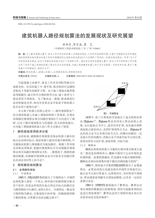
科技与创新｜Science and Technology & Innovation2024年第02期DOI：10.15913/ki.kjycx.2024.02.016建筑机器人路径规划算法的发展现状及研究展望唐维宏，李家盛，董艺（中建四局工程技术研究院，广东广州510665）摘要：为了解决混凝土整平、抹光工序中存在的机器人行驶路径混乱、工作时间难控制问题，从基于传感器对未知环境检测的局部路径规划算法和基于现有环境模型的全局路径规划算法2个方向调研了现有的一些路径规划算法。

列举了2个方向的具体规划算法，并对不同算法的优缺点进行了详细的分析。

最后结合现有的混凝土整平、抹光工序中的特殊工作环境分析了适用于施工现场的机器人算法及对未来的展望，为施工现场建筑机器人的工作方式提供一定的参考价值，提升了建筑施工中的智能化、高效化水平。

关键词：移动机器人；混凝土机器人；全局路径规划；局部路径规划中图分类号：TP242 文献标志码：A 文章编号：2095-6835（2024）02-0060-03目前混凝土的整平、抹光工序多采用桁驾驶式汽油抹光机。

在实际施工中，整平机、抹光机的行走路线多取决于驾驶员的操作习惯。

由于施工现场未提供规范驾驶路径，缺乏科学合理的指导方法，施工效率与工程品质得不到保证。

为了解决这一难题，推动建筑行业的智能化变革，国内外多家企业开始着手将机器人技术应用于建筑行业[1]。

本文基于机器人的核心技术——路径规划算法[2]，结合建筑机器人在施工现场的特殊工作场景，分别从局部路径规划算法和全局路径规划2个方向进行了调研，讨论了路径规划算法与传感器、语义的深度融合，并对施工现场建筑机器人的工作方式提出了展望。

1 路径规划常用技术分类总的来说，避障路径规划要求保证机器人能从初始点运动到目标点，保证机器人能实时避开障碍物，尽可能保证机器人规划路径为最短路径。

根据工作环境及具体适用场景，把路径规划算法分为局部路径规划算法和全局路径规划算法2类。

Optimal and efficient path planning for partially known environments

Optimal and Efﬁcient Path Planning for Partially-Known EnvironmentsAnthony StentzThe Robotics Institute; Carnegie Mellon University; Pittsburgh, PA 15213AbstractThe task of planning trajectories for a mobile robot has received considerable attention in the research literature. Most of the work assumes the robot has a complete and accurate model of its environment before it begins to move; less attention has been paid to the problem of partially known environments. This situation occurs for an exploratory robot or one that must move to a goal location without the benefit of a floorplan or terrain map. Existing approaches plan an initial path based on known information and then modify the plan locally or replan the entire path as the robot discovers obstacles with its sensors, sacriﬁcing optimality or computational efﬁciency respectively. This paper introduces a new algorithm, D*, capable of planning paths in unknown, partially known, and changing environments in an efficient, optimal, and complete manner.1.0IntroductionThe research literature has addressed extensively the motion planning problem for one or more robots moving through a ﬁeld of obstacles to a goal. Most of this work assumes that the environment is completely known before the robot begins its traverse (see Latombe [4] for a good survey). The optimal algorithms in this literature search a state space (e.g., visibility graph, grid cells) using the dis-tance transform [2] or heuristics [8] to ﬁnd the lowest cost path from the robot’s start state to the goal state. Cost can be deﬁned to be distance travelled, energy expended, time exposed to danger, etc.Unfortunately, the robot may have partial or no information about the environment before it begins its traverse but is equipped with a sensor that is capable of measuring the environment as it moves. One approach to path planning in this scenario is to generate a “global”path using the known information and then attempt to “locally” circumvent obstacles on the route detected by the sensors [1]. If the route is completely obstructed, a new global path is planned. Lumelsky [7] initially assumes the environment to be devoid of obstacles and moves the robot directly toward the goal. If an obstacle obstructs the path, the robot moves around the perimeter until the point on the obstacle nearest the goal is found. The robot then proceeds to move directly toward the goal again. Pirzadeh [9] adopts a strategy whereby the robot wanders about the environment until it discovers the goal. The robot repeatedly moves to the adjacent location with lowest cost and increments the cost of a location each time it visits it to penalize later traverses of the same space. Korf [3] uses initial map information to estimate the cost to the goal for each state and efﬁciently updates it with backtracking costs as the robot moves through the environment.While these approaches are complete, they are also suboptimal in the sense that they do not generate the lowest cost path given the sensor information as it is acquired and assuming all known, a priori information is correct. It is possible to generate optimal behavior by computing an optimal path from the known map information, moving the robot along the path until either it reaches the goal or its sensors detect a discrepancy between the map and the environment, updating the map, and then replanning a new optimal path from the robot’s current location to the goal. Although this brute-force, replanning approach is optimal, it can be grossly inefficient, particularly in expansive environments where the goal is far away and little map information exists. Zelinsky [15] increases efficiency by using a quad-tree [13] to represent free and obstacle space, thus reducing the number of states to search in the planning space. For natural terrain, however, the map can encode robot traversability at each location ranging over a continuum, thus rendering quad-trees inappropriate or suboptimal.This paper presents a new algorithm for generating optimal paths for a robot operating with a sensor and a map of the environment. The map can be complete, empty, or contain partial information about the environment. ForIn Proceedings IEEE International Conference on Robotics and Automation, May 1994.regions of the environment that are unknown, the map may contain approximate information, stochastic models for occupancy, or even a heuristic estimates. The algorithm is functionally equivalent to the brute-force,optimal replanner, but it is far more efﬁcient.The algorithm is formulated in terms of an optimal find-path problem within a directed graph, where the arcs are labelled with cost values that can range over a continuum. The robot’s sensor is able to measure arc costs in the vicinity of the robot, and the known and estimated arc values comprise the map. Thus, the algorithm can be used for any planning representation, including visibility graphs [5] and grid cell structures. The paper describes the algorithm, illustrates its operation, presents informal proofs of its soundness, optimality, and completeness, and then concludes with an empirical comparison of the algorithm to the optimal replanner.2.0The D* AlgorithmThe name of the algorithm, D*, was chosen because it resembles A* [8], except that it is dynamic in the sense that arc cost parameters can change during the problem-solving process. Provided that robot motion is properly coupled to the algorithm, D* generates optimal trajecto-ries. This section begins with the deﬁnitions and notation used in the algorithm, presents the D* algorithm, and closes with an illustration of its operation.2.1DeﬁnitionsThe objective of a path planner is to move the robot from some location in the world to a goal location, such that it avoids all obstacles and minimizes a positive cost metric (e.g., length of the traverse). The problem space can be formulated as a set of states denoting robot loca-tions connected by directional arcs , each of which has an associated cost. The robot starts at a particular state and moves across arcs (incurring the cost of traversal) to other states until it reaches the goal state, denoted by . Every state except has a backpointer to a next state denoted by . D* uses backpointers to represent paths to the goal. The cost of traversing an arc from state to state is a positive number given by the arc cost function . If does not have an arc to , then is undeﬁned. Two states and are neighbors in the space if or is deﬁned.Like A*, D* maintains an list of states. The list is used to propagate information about changes to the arc cost function and to calculate path costs to states in the space. Every state has an associated tag ,such that if has never been on the list, if is currently on the list, andG X G Y b X ()Y =Y X c X Y ,()Y X c X Y ,()X Y c X Y ,()c Y X ,()OPEN OPEN X t X ()t X ()NEW =X OPEN t X ()OPEN =XOPEN if is no longer on the list. For each state , D* maintains an estimate of the sum of the arc costs from to given by the path cost function . Given the proper conditions, this estimate is equivalent to the optimal (minimal) cost from state to , given by the implicit function . For each state on the list (i.e.,), the key function,, is defined to be equal to the minimum of before modification and all values assumed by since was placed on the list. The key function classiﬁes a state on the list into one of two types:a state if , and a state if . D* uses states on the listto propagate information about path cost increases (e.g.,due to an increased arc cost) and states to propagate information about path cost reductions (e.g.,due to a reduced arc cost or new path to the goal). The propagation takes place through the repeated removal of states from the list. Each time a state is removed from the list, it is expanded to pass cost changes to its neighbors. These neighbors are in turn placed on the list to continue the process.States on the list are sorted by their key function value. The parameter is defined to be for all such that . The parameter represents an important threshold in D*: path costs less than or equal to are optimal, and those greater than may not be optimal. The parameter is deﬁned to be equal to prior to most recent removal of a state from the list. If no states have been removed,is undeﬁned.An ordering of states denoted by is defined to be a sequence if for all such that and for all such that . Thus, a sequence deﬁnes a path of backpointers from to . A sequence is defined to be monotonic if( a n d) o r ( and ) for all such that . D* constructs and maintains a monotonic sequence , representing decreasing current or lower-bounded path costs, for each state that is or was on the list. Given a sequence of states , state is an ancestor of state if and a descendant of if .For all two-state functions involving the goal state, the following shorthand notation is used:.Likewise, for sequences the notation is used.The notation is used to refer to a function independent of its domain.t X ()CLOSED =X OPEN X X G h G X ,()X G o G X ,()X OPEN t X ()OPEN =k G X ,()h G X ,()h G X ,()X OPEN X OPEN RAISE k G X ,()h G X ,()<LOWER k G X ,()h G X ,()=RAISE OPEN LOWER OPEN OPEN OPEN k min min k X ()()X t X ()OPEN =k min k min k min k old k min OPEN k old X 1X N {,}b X i 1+()X i =i 1i ≤N <X i X j ≠i j (,)1i ≤j <N ≤X N X 1X 1X N {,}t X i ()CLOSED =h G X i ,()h G X i 1+,()<t X i ()OPEN =k G X i ,()h G X i 1+,()<i 1i ≤N <G X {,}X OPEN X 1X N {,}X i X j 1i j N ≤<≤X j 1j i N ≤<≤f X ()f G X ,()≡X {}G X {,}≡f °()2.2Algorithm DescriptionThe D* algorithm consists primarily of two functions: and .is used to compute optimal path costs to the goal, and is used to change the arc cost function and enter affected states on the list. Initially, is set to for all states,is set to zero, and is placed on the list. The ﬁrst function,, is repeatedly called until the robot’s state,, is removed from the list (i.e.,) or a value of -1 is returned, at which point either the sequence has been computed or does not exist respectively. The robot then proceeds to follow the backpointers in the sequence until it eitherreaches the goal or discovers an error in the arc cost func-tion (e.g., due to a detected obstacle). The second function,, is immediately called to cor-rect and place affected states on the list. Let be the robot’s state at which it discovers an error in .By calling until it returns ,the cost changes are propagated to state such that . At this point, a possibly new sequence has been constructed, and the robot continues to follow the backpointers in the sequence toward the goal.T h e a l g o r i t h m s f o r a n d are presented below. The embedded routines are , which returns the state on the list with minimum value ( if the list is empty);, which returns for the list (-1 if the list is empty);, which deletes state from the list and sets ; and , w h i c h c o m p u t e s i f , if , and i f , s e t s and , and places or re-positions state on the list sorted by .In function at lines L1 through L3,the state with the lowest value is removed from the list. If is a state (i.e.,), its path cost is optimal since is equal to the old . At lines L8 through L13, each neighbor of is examined to see if its path cost can be lowered. Additionally,neighbor states that are receive an initial path cost value, and cost changes are propagated to each neighbor that has a backpointer to , regardless of whether the new cost is greater than or less than the old. Since these states are descendants of , any change to the path cost of affects their path costs as well. The backpointer of is redirected (if needed) so that the monotonic sequence is constructed. All neighbors that receive a new pathPROCESS STATE –MODIFY COST –PROCESS STATE –MODIFY COST –c °()OPEN t °()NEW h G ()G OPEN PROCESS STATE –X OPEN t X ()CLOSED =X {}X {}c °()MODIFY COST –c °()OPEN Y c °()PROCESS STATE –k min h Y ()≥Y h Y ()o Y ()=Y {}PROCESS STATE –MODIFY COST –MIN STATE –OPEN k °()NULL GET KMIN –k min OPEN DELETE X ()X OPEN t X ()CLOSED =INSERT X h new ,()k X ()h new =t X ()NEW =k X ()min k X ()h new ,()=t X ()OPEN =k X ()min h X ()h new ,()=t X ()CLOSED =h X ()h new =t X ()OPEN =X OPEN k °()PROCESS STATE –X k °()OPEN X LOWER k X ()h X ()=h X ()k min Y X NEW Y X X X Y Y {}cost are placed on the list, so that they will propagate the cost changes to their neighbors.If is a state, its path cost may not be optimal.Before propagates cost changes to its neighbors, its optimal neighbors are examined at lines L4 through L7 to see if can be reduced. At lines L15 through L18, cost changes are propagated to states and immediate descendants in the same way as for states. If is able to lower the path cost of a state that is not an immediate descendant (lines L20 and L21), is placed back on the list for future expansion. It is shown in the next section that this action is required to avoid creating a closed loop in the backpointers. If the path cost of is able to be reduced by a suboptimal neighbor (lines L23 through L25), the neighbor is placed back on the list. Thus, the update is “postponed” until the neighbor has an optimal path cost.Function: PROCESS-STATE ()L1L2if then return L3;L4if then L5for each neighbor of :L6if and then L7;L8if then L9for each neighbor of :L10if or L11( and ) or L12( and ) then L13;L14else L15for each neighbor of :L16if or L17( and ) then L18;L19else L20if and then L21L22else L23if and and L24 and then L25L26return OPEN X RAISE X h X ()NEW LOWER X X OPEN X OPEN X MIN STATE ()–=X NULL =1–k old GET KMIN –()=DELETE X ()k old h X ()<Y X h Y ()k old ≤h X ()h Y ()c Y X ,()+>b X ()Y =h X ()h Y ()c Y X ,()+=k old h X ()=Y X t Y ()NEW =b Y ()X =h Y ()h X ()c X Y ,()+≠b Y ()X ≠h Y ()h X ()c X Y ,()+>b Y ()X =INSERT Y h X ()c X Y ,()+,()Y X t Y ()NEW =b Y ()X =h Y ()h X ()c X Y ,()+≠b Y ()X =INSERT Y h X ()c X Y ,()+,()b Y ()X ≠h Y ()h X ()c X Y ,()+>INSERT X h X (),()b Y ()X ≠h X ()h Y ()c Y X ,()+>t Y ()CLOSED =h Y ()k old >INSERT Y h Y (),()GET KMIN ()–In function , the arc cost function is updated with the changed value. Since the path cost for state will change, is placed on the list. When is expanded via , it computes a new and places on the list.Additional state expansions propagate the cost to the descendants of .Function: MODIFY-COST (X, Y, cval)L1L2if then L3return 2.3Illustration of OperationThe role of and states is central to the operation of the algorithm. The states (i.e.,) propagate cost increases, and the states (i.e.,) propagate cost reductions. When the cost of traversing an arc is increased, an affected neighbor state is placed on the list, and the cost increase is propagated via states through all state sequences containing the arc. As the states come in contact with neighboring states of lower cost, these states are placed on the list, and they sub-sequently decrease the cost of previously raised states wherever possible. If the cost of traversing an arc isdecreased, the reduction is propagated via states through all state sequences containing the arc, as well as neighboring states whose cost can also be lowered.Figure 1: Backpointers Based on Initial PropagationFigure 1 through Figure 3 illustrate the operation of the algorithm for a “potential well” path planning problem.MODIFY COST –Y X OPEN X PROCESS STATE –h Y ()h X ()c X Y ,()+=Y OPEN Y c X Y ,()cval=t X ()CLOSED =INSERT X h X (),()GET KMIN ()–RAISE LOWER RAISE k X ()h X ()<LOWER k X ()h X ()=OPEN RAISE RAISE LOWER OPEN LOWER GThe planning space consists of a 50 x 50 grid of cells .Each cell represents a state and is connected to its eight neighbors via bidirectional arcs. The arc cost values are small for the cells and prohibitively large for the cells.1 The robot is point-sized and is equipped with a contact sensor. Figure 1 shows the results of an optimal path calculation from the goal to all states in the planning space. The two grey obstacles are stored in the map, but the black obstacle is not. The arrows depict the backpointer function; thus, an optimal path to the goal for any state can be obtained by tracing the arrows from the state to the goal. Note that the arrows deflect around the grey, known obstacles but pass through the black,unknown obstacle.Figure 2: LOWER States Sweep into WellThe robot starts at the center of the left wall and follows the backpointers toward the goal. When it reaches the unknown obstacle, it detects a discrepancy between the map and world, updates the map, colors the cell light grey, and enters the obstacle cell on the list.Backpointers are redirected to pull the robot up along the unknown obstacle and then back down. Figure 2illustrates the information propagation after the robot has discovered the well is sealed. The robot’s path is shown in black and the states on the list in grey.states move out of the well transmitting path cost increases. These states activate states around the1. The arc cost value of OBSTACLE must be chosen to be greater than the longest possible sequence of EMPTY cells so that a simple threshold can be used on the path cost to determine if the optimal path to the goal must pass through an obstacle.EMPTY OBSTACLE GLOWER statesRAISE statesLOWER statesOPEN OPEN RAISE LOWER“lip” of the well which sweep around the upper and lower obstacles and redirect the backpointers out of the well.Figure 3: Final Backpointer ConﬁgurationThis process is complete when the states reach the robot’s cell, at which point the robot moves around the lower obstacle to the goal (Figure 3). Note that after the traverse, the backpointers are only partially updated.Backpointers within the well point outward, but those in the left half of the planning space still point into the well.All states have a path to the goal, but optimal paths are computed to a limited number of states. This effect illustrates the efficiency of D*. The backpointer updates needed to guarantee an optimal path for the robot are limited to the vicinity of the obstacle.Figure 4 illustrates path planning in fractally generated terrain. The environment is 450 x 450 cells. Grey regions are fives times more difficult to traverse than white regions, and the black regions are untraversible. The black curve shows the robot’s path from the lower left corner to the upper right given a complete, a priori map of the environment. This path is referred to as omniscient optimal . Figure 5 shows path planning in the same terrain with an optimistic map (all white). The robot is equipped with a circular field of view with a 20-cell radius. The map is updated with sensor information as the robot moves and the discrepancies are entered on the list for processing by D*. Due to the lack of a priori map information, the robot drives below the large obstruction in the center and wanders into a deadend before backtracking around the last obstacle to the goal. The resultant path is roughly twice the cost of omniscientGLOWER OPEN optimal. This path is optimal, however, given the information the robot had when it acquired it.Figure 4: Path Planning with a Complete MapFigure 5: Path Planning with an Optimistic MapFigure 6 illustrates the same problem using coarse map information, created by averaging the arc costs in each square region. This map information is accurate enough to steer the robot to the correct side of the central obstruction, and the resultant path is only 6% greater incost than omniscient optimal.Figure 6: Path Planning with a Coarse-Resolution Map3.0Soundness, Optimality, andCompletenessAfter all states have been initialized to and has been entered onto the list, the function is repeatedly invoked to construct state sequences. The function is invoked to make changes to and to seed these changes on the list. D* exhibits the following properties:Property 1: If , then the sequence is constructed and is monotonic.Property 2: When the value returned by e q u a l s o r e x c e e d s , t h e n .Property 3: If a path from to exists, and the search space contains a finite number of states, will be c o n s t r u c t e d a f t e r a fi n i t e n u m b e r o f c a l l s t o . I f a p a t h d o e s n o t e x i s t , will return -1 with .Property 1 is a soundness property: once a state has been visited, a finite sequence of backpointers to the goal has been constructed. Property 2 is an optimality property.It defines the conditions under which the chain of backpointers to the goal is optimal. Property 3 is a completeness property: if a path from to exists, it will be constructed. If no path exists, it will be reported ina finite amount of time. All three properties holdX t X ()NEW =G OPEN PROCESS STATE –MODIFY COST –c °()OPEN t X ()NEW ≠X {}k min PROCESS STATE –h X ()h X ()o X ()=X G X {}PROCESS STATE –PROCESS STATE –t X ()NEW =X G regardless of the pattern of access for functions and .For brevity, the proofs for the above three properties are informal. See Stentz [14] for the detailed, formal p r o o f s. C o n s i d e r P r o p e r t y 1 fi r s t. W h e n e v e r visits a state, it assigns to point to an existing state sequence and sets to preserve monotonicity. Monotonic sequences are subsequently manipulated by modifying the functions ,,, and . When a state is placed on the list (i.e.,), is set to preserve monotonicity for states with backpointers to .Likewise, when a state is removed from the list, the values of its neighbors are increased if needed to preserve monotonicity. The backpointer of a state ,, can only be reassigned to if and if the sequence contains no states. Since contains no states, the value of every state in the sequence must be less than . Thus, cannot be an ancestor of , and a closed loop in the backpointers cannot be created.Therefore, once a state has been visited, the sequence has been constructed. Subsequent modifications ensure that a sequence still exists.Consider Property 2. Each time a state is inserted on or removed from the list, D* modifies values so that for each pair of states such that is and is . Thus, when is chosen for expansion (i.e.,), the neighbors of cannot reduce below , nor can the neighbors, since their values must be greater than . States placed on the list during the expansion of must have values greater than ; thus, increases or remains the same with each invocation of . If states with values less than or equal to are optimal, then states with values between (inclusively) and are optimal, since no states on the list can reduce their path costs. Thus, states with values less than or equal to are optimal. By induction,constructs optimal sequences to all reachable states. If the a r c c o s t i s m o d i fi e d , t h e f u n c t i o n places on the list, after which is less than or equal to . Since no state with can be affected by the modified arc cost, the property still holds.Consider Property 3. Each time a state is expanded via , it places its neighbors on the list. Thus, if the sequence exists, it will be constructed unless a state in the sequence,, is never selected for expansion. But once a state has been placedMODIFY COST –PROCESS STATE –PROCESS STATE –NEW b °()h °()t °()h °()k °()b °()X OPEN t X ()OPEN =k X ()h X ()X X h °()X b X ()Y h Y ()h X ()<Y {}RAISE Y {}RAISE h °()h Y ()X Y X X {}X {}OPEN h °()k X ()h Y ()c Y X ,()+≤X Y ,()X OPEN Y CLOSED X k min k X ()=CLOSED X h X ()k min OPEN h °()k min OPEN X k °()k X ()k min PROCESS STATE –h °()k old h °()k old k min OPEN h °()k min PROCESS STATE –c X Y ,()MODIFY COST –X OPEN k min h X ()Y h Y ()h X ()≤PROCESS STATE –NEW OPEN X {}Yon the list, its value cannot be increased.Thus, due to the monotonicity of , the state will eventually be selected for expansion.4.0Experimental ResultsD* was compared to the optimal replanner to verify its optimality and to determine its performance improve-ment. The optimal replanner initially plans a single path from the goal to the start state. The robot proceeds to fol-low the path until its sensor detects an error in the map.The robot updates the map, plans a new path from the goal to its current location, and repeats until the goal isreached. An optimistic heuristic function is used to focus the search, such that equals the “straight-line”cost of the path from to the robot’s location assuming all cells in the path are . The replanner repeatedly expands states on the list with the minimum value. Since is a lower bound on the actual cost from to the robot for all , the replanner is optimal [8].The two algorithms were compared on planning problems of varying size. Each environment was square,consisting of a start state in the center of the left wall and a goal state in center of the right wall. Each environment consisted of a mix of map obstacles (i.e., available to robot before traverse) and unknown obstacles measurable b y t h e r o b o t ’s s e n s o r. T h e s e n s o r u s e d w a s omnidirectional with a 10-cell radial field of view. Figure 7 shows an environment model with 100,000 states. The map obstacles are shown in grey and the unknown obstacles in black.Table 1 shows the results of the comparison for environments of size 1000 through 1,000,000 cells. The runtimes in CPU time for a Sun Microsystems SPARC-10processor are listed along with the speed-up factor of D*over the optimal replanner. For both algorithms, the reported runtime is the total CPU time for all replanning needed to move the robot from the start state to the goal state, after the initial path has been planned. For each environment size, the two algorithms were compared on five randomly-generated environments, and the runtimes were averaged. The speed-up factors for each environment size were computed by averaging the speed-up factors for the ﬁve trials.The runtime for each algorithm is highly dependent on the complexity of the environment, including the number,size, and placement of the obstacles, and the ratio of map to unknown obstacles. The results indicate that as the environment increases in size, the performance of D*over the optimal replanner increases rapidly. The intuitionOPEN k °()k min Y gˆX ()gˆX ()X EMPTY OPEN gˆX ()h X ()+g ˆX ()X X for this result is that D* replans locally when it detects an unknown obstacle, but the optimal replanner generates a new global trajectory. As the environment increases in size, the local trajectories remain constant in complexity,but the global trajectories increase in complexity.Figure 7: Typical Environment for Algorithm ComparisonTable 1: Comparison of D* to Optimal Replanner5.0Conclusions5.1SummaryThis paper presents D*, a provably optimal and efﬁ-cient path planning algorithm for sensor-equipped robots.The algorithm can handle the full spectrum of a priori map information, ranging from complete and accurate map information to the absence of map information. D* is a very general algorithm and can be applied to problems in artiﬁcial intelligence other than robot motion planning. In its most general form, D* can handle any path cost opti-mization problem where the cost parameters change dur-ing the search for the solution. D* is most efﬁcient when these changes are detected near the current starting point in the search space, which is the case with a robot equipped with an on-board sensor.Algorithm 1,00010,000100,0001,000,000Replanner 427 msec 14.45 sec 10.86 min 50.82 min D*261 msec 1.69 sec 10.93 sec 16.83 sec Speed-Up1.6710.1456.30229.30See Stentz [14] for an extensive description of related applications for D*, including planning with robot shape,field of view considerations, dead-reckoning error,changing environments, occupancy maps, potential ﬁelds,natural terrain, multiple goals, and multiple robots.5.2Future WorkFor unknown or partially-known terrains, recentresearch has addressed the exploration and map building problems [6][9][10][11][15] in addition to the path ﬁnding problem. Using a strategy of raising costs for previously visited states, D* can be extended to support exploration tasks.Quad trees have limited use in environments with cost values ranging over a continuum, unless the environment includes large regions with constant traversability costs.Future work will incorporate the quad tree representation for these environments as well as those with binary cost values (e.g., and ) in order to reduce memory requirements [15].Work is underway to integrate D* with an off-road obstacle avoidance system [12] on an outdoor mobile robot. To date, the combined system has demonstrated the ability to find the goal after driving several hundred meters in a cluttered environment with no initial map.AcknowledgmentsThis research was sponsored by ARPA, under contracts “Perception for Outdoor Navigation” (contract number DACA76-89-C-0014, monitored by the US Army TEC)and “Unmanned Ground Vehicle System” (contract num-ber DAAE07-90-C-R059, monitored by TACOM).The author thanks Alonzo Kelly and Paul Keller for graphics software and ideas for generating fractal terrain.References[1] Goto, Y ., Stentz, A., “Mobile Robot Navigation: The CMU System,” IEEE Expert, V ol. 2, No. 4, Winter, 1987.[2] Jarvis, R. A., “Collision-Free Trajectory Planning Using the Distance Transforms,” Mechanical Engineering Trans. of the Institution of Engineers, Australia, V ol. ME10, No. 3, Septem-ber, 1985.[3] Korf, R. E., “Real-Time Heuristic Search: First Results,”Proc. Sixth National Conference on Artiﬁcial Intelligence, July,1987.[4] Latombe, J.-C., “Robot Motion Planning”, Kluwer Aca-demic Publishers, 1991.[5] Lozano-Perez, T., “Spatial Planning: A Conﬁguration Space Approach”, IEEE Transactions on Computers, V ol. C-32, No. 2,February, 1983.OBSTACLE EMPTY [6] Lumelsky, V . J., Mukhopadhyay, S., Sun, K., “Dynamic Path Planning in Sensor-Based Terrain Acquisition”, IEEE Transac-tions on Robotics and Automation, V ol. 6, No. 4, August, 1990.[7] Lumelsky, V . J., Stepanov, A. A., “Dynamic Path Planning for a Mobile Automaton with Limited Information on the Envi-ronment”, IEEE Transactions on Automatic Control, V ol. AC-31, No. 11, November, 1986.[8] Nilsson, N. J., “Principles of Artiﬁcial Intelligence”, Tioga Publishing Company, 1980.[9] Pirzadeh, A., Snyder, W., “A Uniﬁed Solution to Coverage and Search in Explored and Unexplored Terrains Using Indirect Control”, Proc. of the IEEE International Conference on Robot-ics and Automation, May, 1990.[10] Rao, N. S. V ., “An Algorithmic Framework for Navigation in Unknown Terrains”, IEEE Computer, June, 1989.[11] Rao, N.S.V ., Stoltzfus, N., Iyengar, S. S., “A ‘Retraction’Method for Learned Navigation in Unknown Terrains for a Cir-cular Robot,” IEEE Transactions on Robotics and Automation,V ol. 7, No. 5, October, 1991.[12] Rosenblatt, J. K., Langer, D., Hebert, M., “An Integrated System for Autonomous Off-Road Navigation,” Proc. of the IEEE International Conference on Robotics and Automation,May, 1994.[13] Samet, H., “An Overview of Quadtrees, Octrees andRelated Hierarchical Data Structures,” in NATO ASI Series, V ol.F40, Theoretical Foundations of Computer Graphics, Berlin:Springer-Verlag, 1988.[14] Stentz, A., “Optimal and Efﬁcient Path Planning for Unknown and Dynamic Environments,” Carnegie MellonRobotics Institute Technical Report CMU-RI-TR-93-20, August,1993.[15] Zelinsky, A., “A Mobile Robot Exploration Algorithm”,IEEE Transactions on Robotics and Automation, V ol. 8, No. 6,December, 1992.。

英文资讯：平衡可再生能源的成本

Increasing reliance on renewable energies is the way to achieve greater CO2 emission1 sustainability and energy independence. As such energies are yet only available intermittently2 and energy cannot be stored easily, most countries aim tocombine several energy sources. In a new study in EPJ Plus, French scientists have come up with an open source simulation method to calculate the actual cost of relying on a combination of electricity sources. Bernard Bonin from the Atomic Energy Research Centre CEA Saclay, France, and colleagues demonstrate that cost is not directly proportional to the demand level. Although recognised as crude by its creator, this method can be tailored to account for the public's interest-and not solely3 economic performance-when optimising the energy mix. The authors consider wind, solar, hydraulic4, nuclear, coal and gas as potential energy sources. In their model, the energy demand and availability are cast as random5 variables. The authors simulated the behaviour of the mix for a large number of tests of such variables, using so-called Monte-Carlo simulations.For a given mix, they found the energy cost of the mix presents a minimum as a function of the installed power. This means that if it is too large, the fixed6 costs dominate the total and become overwhelming. In contrast, if it is too small, expensive energy sources need to be frequently solicited7.The authors are also able to optimise the energy mix, according to three selected criteria8, namely economy, environment and supply security.The simulation tested on the case of France, based on 2011 data, shows that an optimal9 mix is 2.4 times the average demand in this territory. This mix contains a large amount of nuclear power, and a small amount of fluctuating energies: wind and solar. It is also strongly export-oriented.英语学习方法：1 emissionn.发出物，散发物；发出，散发参考例句：Rigorous measures will be taken to reduce the total pollutant emission.采取严格有力措施，降低污染物排放总量。

基于改进的RRT^()-connect算法机械臂路径规划

随着时代的飞速发展，高度自主化的机器人在人类社会中的地位与作用越来越大。

而机械臂作为机器人的一个最主要操作部件，其运动规划问题，例如准确抓取物体，在运动中躲避障碍物等，是现在研究的热点，对其运动规划的不断深入研究是非常必要的。

机械臂的运动规划主要在高维空间中进行。

RRT （Rapidly-exploring Random Tree）算法[1]基于随机采样的规划方式，无需对构型空间的障碍物进行精确描述，同时不需要预处理，因此在高维空间被广为使用。

近些年人们对于RRT算法的研究很多，2000年Kuffner等提出RRT-connect算法[2]，通过在起点与终点同时生成两棵随机树，加快了算法的收敛速度，但存在搜索路径步长较长的情况。

2002年Bruce等提出了ERRT（Extend RRT）算法[3]。

2006年Ferguson等提出DRRT （Dynamic RRT）算法[4]。

2011年Karaman和Frazzoli提出改进的RRT*算法[5]，在继承传统RRT算法概率完备性的基础上，同时具备了渐进最优性，保证路径较优，但是会增加搜索时间。

2012年Islam等提出快速收敛的RRT*-smart算法[6]，利用智能采样和路径优化来迫近最优解，但是路径采样点较少，使得路径棱角较大，不利于实际运用。

2013年Jordan等通过将RRT*算法进行双向搜索，提出B-RRT*算法[7]，加快了搜索速度。

同年Salzman等提出在下界树LBT-RRT中连续插值的渐进优化算法[8]。

2015年Qureshi等提出在B-RRT*算法中插入智能函数提高搜索速度的IB-RRT*算法[9]。

同年Klemm等结合RRT*的渐进最优和RRT-connect的双向搜基于改进的RRT*-connect算法机械臂路径规划刘建宇，范平清上海工程技术大学机械与汽车工程学院，上海201620摘要：基于双向渐进最优的RRT*-connect算法，对高维的机械臂运动规划进行分析，从而使规划过程中的搜索路径更短，效率更高。

工业机器人外文参考文献

工业机器人外文参考文献工业机器人外文参考文献1. Gao, Y., & Chen, J. (2018). Review of industrial robots for advanced manufacturing systems. Journal of Manufacturing Systems, 48, 144-156.2. Karaman, M., & Frazzoli, E. (2011). Sampling-based algorithms for optimal motion planning. The International Journal of Robotics Research, 30(7), 846-894.3. Khatib, O. (1986). Real-time obstacle avoidance for manipulators and mobile robots. The International Journal of Robotics Research, 5(1), 90-98.4. Lee, J. H., & Kim, E. B. (2019). Energy-efficient path planning for industrial robots considering joint dynamics. Journal of Mechanical Science and Technology, 33(3),1343-1351.5. Li, D., Li, Y., Wang, X., & Li, H. (2019). Design and implementation of a humanoid robot with flexible manipulators. Robotica, 37(12), 2008-2025.6. Liu, Y., Ren, X., & Wang, T. (2019). A novel adaptive fuzzy sliding mode control for a nonholonomic mobile robot. Soft Computing, 23(3), 1197-1209.7. Loh, A. P., & Tan, K. K. (2014). Vision-based controlof industrial robots using an adaptive neural network. Robotics and Computer-Integrated Manufacturing, 30(2), 177-184.8. Niemeyer, G., & Slotine, J. J. (1990). Stable adaptive teleoperation. The International Journal of Robotics Research, 9(1), 85-98.9. Park, J. Y., & Cho, C. H. (2018). Optimal path planning for industrial robots using a hybrid genetic algorithm. International Journal of Precision Engineering and Manufacturing, 19(5), 755-761.10. Wang, Z., Wang, X., & Liu, Y. (2019). Design and analysis of a novel humanoid robot with intelligent control. International Journal of Advanced Manufacturing Technology, 102(5-8), 1391-1403.。

田作业机械路径优化方法

田作业机械路径优化方法孟志军;刘卉;王华;付卫强【摘要】提出了一种面向农田作业机械的地块全区域覆盖路径优化方法.基于农田地块几何形状、作业机具参数、地头转弯模式等先验信息,将田间作业划分为不同区域,根据选择不同的路径优化目标:转弯数最少、作业消耗最小、总作业路径最短或有效作业路径比最大,计算出最优作业方向,生成最优作业路径.基于地块全区域覆盖路径优化算法,设计开发了农田作业机械的路径规划软件,并选取了4块典型的凸四边形农田地块进行作业路径规划测试.测试结果表明,最优作业方向上的路径优化目标量比其他作业方向上有显著减少;对于上述4个地块,按照不同优化目标计算所得的最优作业方向均与地块某个边的方向角相同,对于长宽比较大的地块,最长边方向通常为最优作业方向.%A kind of optimal path planning method for complete field coverage in agricultural machinery farming was described. The given convex field was decomposed into sub regions according to typical faming pattern of complete field coverage. Optimal path planning should minimize agricultural machines turns, farming time, route distance or other optimization object. According to the different purpose of path planning above, optimal travel direction could be determined based on topological features of arable lands, turns pattern in the headland and other useful information. Fanning path planning software was developed by using this algorithm. The test results from four actual quadrangular fields showed that the optimization object for field operation in optimal travel direction decreased obviously compared with other directions. Each optimal travel direction in those quadrangular fields above was along anyedge-Especially for a quadrangle having a larger edge ratio, the optimal travel direction was almost the longest edge.【期刊名称】《农业机械学报》【年(卷),期】2012(043)006【总页数】6页(P147-152)【关键词】农田作业机械;路径优化;全区域覆盖【作者】孟志军;刘卉;王华;付卫强【作者单位】国家农业信息化工程技术研究中心,北京100097;首都师范大学信息工程学院,北京100048;首都师范大学信息工程学院,北京100048;国家农业信息化工程技术研究中心,北京100097【正文语种】中文【中图分类】S232引言农田作业机械的田间作业路径，一般由操作人员根据习惯、经验和常识性规则进行选择，也有学者提出了一些路径设计方法。

1、下载文档前请自行甄别文档内容的完整性，平台不提供额外的编辑、内容补充、找答案等附加服务。
2、"仅部分预览"的文档,不可在线预览部分如存在完整性等问题,可反馈申请退款(可完整预览的文档不适用该条件!)。
3、如文档侵犯您的权益，请联系客服反馈,我们会尽快为您处理(人工客服工作时间：9:00-18:30)。

Nonlinear Dyn(2014)78:1515–1543DOI10.1007/s11071-014-1532-9ORIGINAL PAPEROptimal path planning of a cable-suspended robot with moving boundary using optimal feedback linearization approachM.H.Korayem·H.Tourajizadeh·A.Zehfroosh·A.H.KorayemReceived:3February2014/Accepted:9June2014/Published online:1July2014©Springer Science+Business Media Dordrecht2014Abstract In this paper,the optimal path of a cable-suspended robot between two boundaries is assessed subject to its maximum load,while the initial and tar-get points are moving boundary.Considering the fact that the most important application of cable robots is load carrying between two boundaries,planning the optimal path in which the heaviest load can be car-ried is extremely applicable.A closed loop optimal path planning algorithm is proposed in this paper for non-linear dynamic of a cable robots based on opti-mal feedback linearization.This method not only pro-duces the optimal path of the end-effector,but also is robust to external disturbances and parametric uncer-tainties as a result of its closed loop nature.Moreover, considering the fact that in many automation applica-tions the target of load handling is a sort of moving boundary like conveyors,ﬁnding the optimal point of this boundary which produces the optimal path with the maximum dynamic load carrying capacity(DLCC) amongst the other points of the boundary is obviously a useful study.Therefore,an online solution,based on variational algorithm is proposed here to solve the moving boundary problem which is compatible with M.H.Korayem(B)·H.Tourajizadeh·A.Zehfroosh·A.H.KorayemRobotics Research Laboratory,Center of Excellencein Experimental Solid Mechanics and Dynamics,School of Mechanical Engineering,Iran Universityof Science and Technology,Tehran,Irane-mail:hkorayem@iust.ac.ir the presented closed loop optimal path planning.This method is developed for both the initial andﬁnal mov-ing boundaries.Finally maximum DLCC is obtained using an iterative method to check the optimality of the proposed method.The efﬁciency of the proposed algo-rithm is veriﬁed at the end by the aid of some simulation scenarios performed on a spatial six DOFs cable robot with six cables.The motors’torque,motors’speed,and resultant DLCCs are calculated for both simple optimal path and moving boundary cases and comparison of the results proves the mentioned claims based on superior-ity of the proposed algorithm of moving boundary in saving the energy and increasing the DLCC.All sim-ulation results are supported by conducting an experi-mental study on the cable robot of IUST(ICaSbot)for regulation movement of the end-effector with moving boundary.Keywords Optimal regulation·Moving boundary·Cable suspended robot·Feedback linearization control·Dynamic load carrying capacity1IntroductionCable robots are considered as a modiﬁed version of cranes in which carrying loads can be controlled bet-ter within its predeﬁned trajectory or point to point movement.Therefore,ﬁnding the maximum load car-rying capacity and its optimal path is deﬁnitely a useful research for industrial environments.However,in order1516M.H.Korayem et al.to neutralize the destructive effect of load swinging, which is common for under constrained cable robots, closed loop optimal control seems to be necessary.As a result not only the stability of the end-effector is assured,but also the optimal path is tracked and so the heaviest load is carried along.To meet this goal a nonlinear controlling algorithm needs to be com-bined with a proper optimizing method.The objec-tive function of this paper should be deﬁned based on required constraints related to maximizing the pay-load.Two dynamic constraints are supposed to be min-imized in this paper including allowable accuracy of the robot,and allowable torque of the motors while the constraint of positive tension of the cables is supposed to be satisﬁed since the robot is maneuvering within its allowable dynamic workspace.Moreover,another geo-metrical constraint for special applications of robots in automation process is considered here which let the system to have even more load carrying capac-ity.In many robotic applications like automation lines, the exact position of the boundary points of the end-effector are not deﬁnitely determined since the load can start or end its movements on a line or a curve which is the conveyor proﬁle of the automation line. This line or curve is called moving boundary of the optimal path.The initial condition of the robot can also be moving boundary in some applications.It is desired that the robot chooses the optimal point of this initial orﬁnal moving boundaries which results in the maximum load carrying capacity.In many automation processes,the gripping and manipulating speed and the speed of placement of the particles on the conveyor is considerably less than the speed of the conveyor.More-over,since the speed of the conveyor is simply control-lable by the aid of an operator,it is always possible to provide a free space on the conveyor through which the particle can be placed in.Thus,it is always pos-sible to have a free space boundary on the conveyor as the start or end point of the robot’s end-effector for which the optimal point can be determined.Therefore, the particle is replaced with considerably less energy while no malfunctionality is occurred on the process of the automation since all of the points of the con-veyors eventually are led to a unique destination.The main purpose of this paper is toﬁnd out the optimal path of the cable robot and its corresponding maxi-mum DLCC between a deﬁnite or moving initial point and a moving boundaryﬁnal point in a closed loop way.Some researchers have been performed in this area so far.The initial researches of optimizations related to the DLCC of the robots are conducted using open loop approaches like Hamilton–Jacobi–Bellman(HJB) method which were not robust to parametric uncertain-ties or external noises.For example,open loop opti-mal control of a spatial cable robot is done by Alp for a six DOFs cable robot with six cables[1]and by Williams for two samples of planar cable robots [2]in order to minimize the cables tension.Applica-tions of cable robots made researchers study differ-ent aspects of them such as dynamic modeling,con-trol strategies,load carrying capacity,accuracy and also designing more efﬁcient cable robots.For exam-ple,Pott et al.introduce a new version of cable driven robot,IPAnema,that has more applications for indus-trial processes[3],or Merlet studied a redundantly actu-ated robot with eight cables[4].Moreover,stability of underconstrained cable driven robot is studied in [5].Accuracy of cable robot while carrying payload, which is one of their important application,is stud-ied and improved by Pott and co-workers[6].Opti-mizing the DLCC of a six cable robot is done by[7] using open loop variational approach.Iterative linear programming(ILP)method is employed by Korayem et al.[8]for the same cable robot in order to maxi-mize the payload of the system.Moreover,the men-tioned cable robot with elastic characteristics is opti-mized in[9]using open loop optimization approach. Considering the fact that in open loop approaches the robustness of the system to disturbances and uncertain-ties is not guaranteed,some algorithms were developed which planed the optimal path under the control of a closed loop system with different objective functions. For example feedback linearization method is used in [10]in order to optimal distributing of cables’tension for a constrained sample of a cable robot by Fang et al.Trevisani has also optimized a constrained sample of cable robot to achieve the minimum cables’tension [11].Optimization of tracking accuracy of a cable robot is performed in[12]using adaptive controller.PD con-troller is used in[13]in order to minimize the motors’torque.Maximizing the load capacity of cable robots as the desired objective function is considered in[14]for a predeﬁned trajectory withﬂexible joints.Also DLCC of a crane is optimized in[15–17]for crane applica-tions using robust controller.State dependent Riccati equation(SDRE)is used in[18]to optimal control of aﬂexible cable transporter system while the stabilityOptimal path planning of a cable-suspended robot with moving boundary1517is guaranteed by robust H-inﬁnity method.The same method(SDRE)is used by Korayem and Zehfroosh for optimal motion planning of cable robot in the pres-ence of obstacles and moving boundaries[19]which is nonlinear with high calculation process and is not proper for real time applications.Korayem and Toura-jizadeh focused on obstacle as a constraint of optimal path planning and proposed a proper strategy to avoid collision and combined this strategy with adaptive opti-mal feedback linearization approach[20].The fact that in some industrial environments the boundaries are not determined as a point,the idea of extra optimization of the robots was ignited in[21]for moving boundary cases but in an open loop way.However,something has not been done yet which is necessary to be considered.In this paper,the lack of [21]i.e.,its open loop nature,is improved.The opti-mal path of a spatial under constrained cable-suspended robot which acts under the control of a closed loop con-troller is assessed while its initial and target points are moving boundary and their related maximum DLCC are also calculated.This goal is satisﬁed in this paper by designing a closed loop optimal strategy combined of feedback linearization controlling method which is a proper controlling strategy for non-linear systems, together with optimizing tool of LQR(linear quadratic regulator)which is a strong optimizing algorithm of linear systems.Destructive effects of nonlinearity of the plant are neutralized by exact linearizing the sys-tem using feedback linearization method.Therefore, stability of the system is guaranteed by Lyapunov and optimality and robustness of the closed loop plant is provided by LQR which has an acceptable phase and gain margins.Thus,contrary to the open loop optimal path planning approaches,not only the optimal path is found in an online way,but also the procedure is robust against any kind of external disturbances and paramet-ric uncertainties since the optimal path is tracked using the actual position feedback of the end-effector.More-over,to solve the moving boundary problem in theﬁnal point,a geometrical based method is proposed accord-ing to variational approach,whichﬁnds the optimal point of any kind of moving boundaries consisting of straight line,curve or surface shaped boundaries for a closed loop system with a fast calculation capabil-ity which is suitable for online processes.Therefore,a complementary algorithm is attached to the designed optimal controller and a method is derived toﬁnd the instantaneous optimal point of the moving boundary in an on line way.This point is fed to the controller as the online setpoint to minimize the consumed energy.Con-sidering the fact that the optimal path of the end-effector is not a straight line,the optimal point is not a constant target and varies during the regulation process.An iter-ative method is also proposed toﬁnd the optimal point of moving boundary at the starting point.Moreover, the effect of gravity on the moving boundary is studied and the efﬁciency of the proposed moving boundary strategy at theﬁnal and initial points is compared.First of all,the non-linear formulation of parallel cable robot are represented and then feedback lineariza-tion is implemented which converts the dynamic into linear state space.Secondly,the proposed closed loop control algorithm is optimized based on LQR.After-ward,the employed iterative algorithm of calculating the maximum load carrying capacity of this system is portrayed based on an objective function consist-ing of end-effector’s error and motors’torque.Finally, the geometrical constraint of DLCC which isﬁnding the optimal point of a moving boundary is then real-ized by proposing a complementary variational based strategy forﬁnal point while an iterative method is derived for initial moving boundary.The efﬁciency of the designed controller and also the proposed algo-rithm of moving boundary problem are veriﬁed by the aid of a series of simulation studies done on a spa-tial six DOFs under constrained cable robot and com-paring the results between the simple system and the one which is equipped by moving boundary strategy. Four different categories of moving boundary problems are studied in this paper including straight line mov-ing boundary,curve and surface shaped samples and ﬁnally a generalized case in which both of initial and ﬁnal points are moving boundaries.The superiority of the closed loop over open loop approaches,the effect of gravity and involved DOFs,differences of initial and ﬁnal moving boundaries and the relation between the torque changes and the distance of theﬁxed setpoint to the optimal one which is calculated by the aid of moving boundary strategy is also investigated in this section.The related optimal DLCC is calculated then and the effect of the proposed algorithm on this objec-tive parameter is analyzed.DLCC is calculated using an iterative method with an analytic approach which is secure from numerical problems or local optimiza-tion syndrome.The effect of the proposed method on the torque and optimal path and eventually its related DLCC is investigated.At the end,all of the theoreti-1518M.H.Korayem et al.cal claims and simulation results are veriﬁed by com-paring them with experimental studies which are con-ducted on the Iran University of Science and Technol-ogy Cable-Suspended Robot(ICaSbot).This robot is an under constrained spatial cable robot with six degrees of freedom and six active cables.The good compatibil-ity of the simulation and experimental results validates the correctness of the proposed algorithm and the opti-mality of the proposed moving boundary strategy is practically investigated.2Optimal feedback linearization formulation Formulation of optimal path planning between two points in a closed loop way and deﬁning its DLCC is presented in this section.The moving boundary con-dition is solved as a new constraint of optimization.2.1Dynamic and optimal control schemeThe“n”notation presents the global coordinate of the robot while the“b”presents its local one.Dynamic equation of an under constrained cable-suspended robot with six DOFs and six supporting cables of Fig.1 can be described as Eq.(1)[1]:D(X)¨X+C(X,˙X)˙X+g(X)=S T J(q(X))T;X={x m,y m,z m,ϕ, ,ψ}(1)where X is the vector of translational and rotational DOFs of the end-effector,T is the tension vector oftheFig.1Spatial sample of cable robot[1]cables,q is the length of the cables m is the load of the end-effector and I is the moment of inertia of the end-effector.Also we have:D=m I300P T I P;C=03P T{I˙P˙o+(P˙o)×I(P o)};g=⎡⎢⎢⎣−mg03⎤⎥⎥⎦;S J=∂q i∂x ji×j;P=⎡⎣10−sinθ0cosψsinψcos0−sinψcosψcos⎤⎦;˙o=⎡⎣˙˙˙ϕ⎤⎦D is the inertia matrix of the robot;C and g are its Cori-olis matrix and gravity vector respectively and S J is the Jacobian matrix.According to[22]using feedback linearization method results in the following required cables’tension and motors’torque:T i=S−T J(D(X)ν+C(X,˙X)+g(X))i⇒τi=r S−T J(Dν+C+g)+J¨β+c˙β;i=1,...6(2) where J is the rotary inertia of the motor,r is the radius of the drum,˙βis its angular velocity,c is the viscose damping of the motor andνis the control input of the outer closed loop of feedback linearization and can be evaluated as below to create a controllable error equa-tion which can be stabilized using LQR:νi=¨X d+K i D(˙X d−˙X a)+K i P(X d−X a);i=1,...,6(3) where K i D and K i P are controlling gains of deriva-tive and proportional errors respectively and should be optimized in order to have an optimal regulation[22]. Indeed,outer closed loop controlling signal deals with converting the non-linear state space of the robot into linearized closed loop state space which can be opti-mized using LQR,while the inner closed loop con-trolling signal is related to calculating the optimized required motors’torque.Based on Eqs.(2,3),the non-linear state space of the cable robot,is converted into linear one which can be stabilized and optimized using proper controlling gains by the aid of LQR.The control procedure can be shown in Fig.2.Since the related state space is linearized,it is pos-sible to use LQR to optimize the controlling gains.ToOptimal path planning of a cable-suspended robot with moving boundary1519Fig.2Control procedure of the robot based on optimal feedback linearizationachieve this goal,the constraints which are involved in optimizing the objective function should be deter-mined.Two main constraints of calculating the DLCC of a robot including required motors’torque and track-ing error are supposed to be minimized by the aid of LQR method in order to obtain the maximum load capacity.So,the cost function can be deﬁned as below:J L Q R (X ,t )=∞t(e r (X ,t )T Qe r (X ,t )+u (X ,t )T Ru (X ,t ))d τ(4)where e r is the error of the state space of the system,Q is the penalty matrix of accuracy,R is the penalty matrix of control input and u is controlling input.Solv-ing this cost function results in the Ricatti equation in which its stability is also assured by the aid of Lyaponov Equation [23].Finally solving the mentioned Riccati equation results in the following optimal control input:u ∗=−R −1B T Se r (X ,t )=−R −1B T S [e ;˙e](5)where e and ˙e are the error of position and velocityrespectively,S is the resultant of Riccati equation and B is the controlling matrix of the linearized state space.This obtained optimal value u ∗should be substituted in the last two terms of Eq.(3)to calculate the linearized optimal controlling input.νio=¨X id −R −1B T Se r (X ,t )⇒τio =r S −T JD ¨X id −R −1B T Se r (X ,t ) +C +g +J ¨β+C ˙β;i =1,...6(6)In a regulation process the setpoint is constant so,wehave ¨Xd =0.Also other matrices of the controlling vector in a regulation process should be substituted using feed forward terms of inverse dynamics.Thus,by optimizing the controlling gains,whole the controlling input will be optimized and the resultant path which is tracked by this control signal will be the optimum one:X o =1D (X ) −C (X ,˙X )˙X −g (X )+S J J −T (D (X )(v o )+C (X ,˙X )+g (X ))d t (7)where X o is the optimal path and v o is the optimalcontrolling signal.As a result,a closed loop optimal path planning is provided using feedback linearization together with LQR,by which both the optimality and stability are provided.The moving boundary constraint is also satisﬁed in the next section.2.2DLCC formulationIn this section,the goal is to deﬁne the optimal DLCC of the robot based on the motors’torque constraint,accuracy constraint and moving boundaries constraint.Considering the fact that for an under constrained cable robot there is no remedy to guide the end-effector along a path with negative cable’s tension,the positive ten-sion of the cables are supposed to be satisﬁed since the robot is considered to be operating within its allowable dynamic workspace.In [14]the required iterative method was presented to ﬁnd the DLCC of a robot based on torque and error1520M.H.Korayem et al. Fig.3Flowchart ofdetermining the DLCC of aclose loop cable robotconsidering movingboundaryconstraints.This method is modiﬁed for the closed loop form and considering boundary constraint.Theﬁnal algorithm can be explained like theﬂowchart of Fig.3. The maximum DLCC is estimated by the aid of an itera-tive procedure.In this closed loop approach,the torque and accuracy constraints should be satisﬁed simulta-neously afterﬁnding the optimal point of the moving boundary in order to extract the maximum DLCC.The payload of the system after deﬁning the optimal point of the moving boundary is increased gradually in an iteration loop as long as theﬁrst constraint is violated. The penalty gains of error and controlling input in the objective function of Eq.(4)should be set by the aid of LQR in a way that result in simultaneous satura-tion of torque and accuracy to have the highest DLCC. So,the procedure in each iteration,is a pure analytic approach which is applicable in online regulation and is secure from numerical problems or local optimiza-tion syndromes.It is good to note that,only the process ofﬁnding the maximum DLCC is iterative,and this process do not affect the proposed optimal closed loop control method described in Sect.2.2and Fig.3.Thus, the proposed optimal path planning process with mov-ing boundary and regulation method of control proce-dure is completely on-line which is safe from iterative destructive effects.2.2.1Allowable motors’torque and accuracyconstraintsThe constraints for estimating the DLCC includes two dynamic constraints i.e.,allowable motors’torque and allowable accuracy of the end-effectors and a geomet-rical constraint which is moving boundary condition of the end-effector.The motor torque constraint restricts the applied torque within the allowable bounds of the motor and accuracy constraint restricts the end-effector within its predeﬁned allowable error bounds which should be deﬁned by the operator.The coefﬁcient of these two constraints and their effects on the DLCC of the robots are studied in[14].Optimal path planning of a cable-suspended robot with moving boundary 15212.2.2Straight line moving boundaryIn this section it is supposed that the second bound-ary of the optimal path is not a determined point and is substituted by a line.It is expected that the designed optimal controller ﬁnds its optimal way toward the spe-cial point of this moving boundary for which the max-imum load capacity is achieved.A typical sample of this situation is the automation lines in which the grip-per is supposed to transfer the product from a speciﬁc initial point toward a point on the conveyor line which can be treated as the moving boundary.Considering the fact that the destination of all of the points of the moving line in a conveyor is a unique target,the loca-tion of the second point is not important for the object.However,choosing the point of the automation line for which the heaviest load can be carried is a privilege.It is shown in [21]that whenever an objective func-tion (F (t ,y 1,y 2...,y n ,y 1,y 2,...,y n ))like Eq.(8a )is supposed to be optimized and its ﬁnal point is a mov-ing boundary (g (t ,y 1f ,y 2f ,...y n f )),the condition of Eq.(8b )should be satisﬁed based on variational prin-ciple:I =BAF (t ,y 1,y 2...,y n ,y 1,y 2,...,yn )d t ;yi =d y i /d t (8a)F −n i =1y i ∂F ∂y i t =t f δt f + n i =1∂F ∂yi t =t fδy i f =0(8b)where y 1,...,y n are the DOFs of the end-effector.Forthe closed loop condition in which the objective func-tion of LQR is supposed to be satisﬁed,and considering the paths with the same time duration (δt f =0)substi-tuting the LQR objective function in the above equation results in:6 i =1∂F∂X i δX f =0;X =[x ;y ;z ;ψ;θ;φ](9)where X f is the coordinate of the ﬁnal point of the end-effector on the moving boundary.The mentioned equa-tion should be solved to ﬁnd out the optimal point of the moving boundary which needs slightly a heavy cal-culation.However,based on the mentioned proposed controlling strategy in which the motors’torque are deﬁned based on feedback linearization and are opti-mized based on LQR,the functional of LQR (Eq.(4))can be rewritten as Eq.(12)in which the controlling input is substituted by Eq.(6).According to Eqs.(2,3)we have the following error equation for the closed loop system:¨e i +K D ˙ei +K P e i =0;i =1,...6⇒e i =e λj t;λj = −K i P +− K 2i P −4K i D /2(10)Thus:˙e i = λj e λj t ⇒˙e=f (e )(11)And so,the objective function is purely a polynomial function of single term of DOFs error:F (X ,t )=e r (f (e ))T Qe r (f (e ))+(K i D (f (e ))+K i P (e ))TR (K i D (f (e ))+K i P (e ))F =f (e )⇒e →min(12)where e r is the vector including e and ˙e .Base on Eq.(8),time (t)is the independent variable,error and itsderivatives are the dependent variables (y =e ;y =˙e).Substituting the above functional in Eq.(8)and con-sidering the fact that the error’s derivative are also a function of error vector,illustrate that the error vector needs to be minimized in order to satisfy the moving boundary condition and obtaining the minimal motors’torque.It means that based on the proposed regulation process the strategy of ﬁnding the optimal path is eas-ier with less calculation process which is applicable for on-line robotic applications.In other words,it is math-ematically proved that in order to ﬁnd the optimal point of a moving boundary it is sufﬁcient to ﬁnd the nearest point of the moving boundary to the instantaneous posi-tion of the end effector for each time interval instead of solving the heavy calculation of the Eq.(9).The nearest point of the moving boundary doesn’t remain a unique point during the whole period of end-effectors’movement since the optimal path of a non-linear system for a determined target point is not a straight line and changes during the time based on the objective func-tion which itself is a function of non-linear dynamics of the robot.Therefore,the instantaneous setpoint of the end-effector is not constant and should be calculated versus the time.Also,as it was proved,the nearest point should be found respect to this actual position of the end-effector since whole the objective function for the proposed regulation strategy is a function of error.As a result of minimizing the mentioned objective function,controlling input which is the motors’torque is mini-mized together with the state error which is related to the end-effector displacement or motor speed.Thus,the power which is the multiplication of these two parame-ters is minimized by the proposed optimal regulation1522M.H.Korayem et al. with moving boundaries which consequently results inoptimizing the consumed energy.Three different cases are considered for the movingboundary problem.First a straight line is assumed as anopen loop curve of moving boundary.In order to deﬁnethe nearest point of this line with respect to instanta-neous position of the end-effector,it is sufﬁcient toﬁndthe orthogonal projection of the instantaneous positionof the end-effector on the moving boundary line(X f):X f=X1l+ 3j=1((−(X2l(j)−X1l(j))∗(X1l(j)−X e(j)) 3j=1(X2l(j)−X1l(j))2∗(X2l(j)−X1l(j));X={x;y;z;ϕ;θ;φ}(13) where X1l and X2l are the initial andﬁnal points of the straight moving boundary line,X e is the instantaneous position of the end-effector and X f is the instanta-neous optimal setpoint of the end-effector on the mov-ing boundary.Since the moving boundary is not a line but a segment of a line as an open loop curve,the cal-culated setpoint can be located within the segment or along it.This fact affects on the choosing the instanta-neous setpoint of the end-effector.To verify this prob-lem it should be considered that if the following condi-tion is satisﬁed,the setpoint is within the segment of the line and therefore,can be treated as the instantaneous setpoint of the end-effector:(X f−x1l)(X f−x2l)<0(14) Otherwise,if the above condition is not satisﬁed,the setpoint is out of the line segment or along the line. In this situation the nearest point to the instantaneous position of the end-effector which should be considered as the new setpoint is one of the two end-sides of the line segment.Therefore,it is sufﬁcient to calculate these two distances and choose the shorter one as the new setpoint of the end-effector.Given the mentioned explanations,it is required to update the setpoint of the regulation process based on the moving boundary strategy to feedback the nearest optimal point of the moving boundary to instantaneous position of the end-effector as the desired setpoint.This new setpoint should be calculated using the instan-taneous position of the end-effector thus,this updat-ing needs the actual position of the end-effector which should be provided by the aid of sensors.Thus,this upgrading should be performed in each time interval of controlling procedure which depends on the sam-pling rate of the installed sensors.In the experimental study(and also simulation),the sample rate is consid-ered0.01second so,the upgrading rate of the setpoint is done each0.01second.(Encoders are2400pulse per revolution and camera is24frames per second). The strategy of deﬁning the optimal setpoint is shown in Fig.4for eachcase.Fig.4Methodology ofﬁnding the instantaneous optimal setpoint for straight line(left)and curve(right)。