数据库系统概论第二章习部分题解
数据库系统概论,习题答案详解

本章的知识点数据、数据库、数据库管理系统、数据库系统等概念数据管理技术的三个阶段(优缺点)数据结构化的含义及其方法数据独立性、物理独立性、逻辑独立性数据库系统特点数据描述、建模过程概念数据模型及其设计结构数据模型(逻辑模型)及其三要素:数据结构、数据操作、数据约束条件层次模型概念及其特点、网状模型概念及其特点关系模型概念及其特点模式的概念、数据库三级模式结构、两级映像客户/服务器结构(C/S)数据库系统组成需重点理解掌握的内容:数据结构化数据库系统特点数据独立性概念模型及其设计数据库三级模式结构关系模型作业参考答案:11、解题方法:1、识别实体型及其属性(下划线为实体码)系:系编号,系名,电话教研室:编号,地址教员:工号,姓名,性别,职称班级:班号学生:学号,姓名,性别,层次课程:课程号,课程名“学校”作为限定词不作为实体;“教授/副教授”作为“教员”特例不作为单独实体,必须加上“职称”属性;“研究生”作为“学生”特例不作为单独实体,必须加上“层次”属性。
2、确定实体间联系,包括联系名、类型及其联系属性系与教研室之间存在1:n的“设立”联系。
教研室与教员之间存在1:n的“管理”联系。
系与班级之间存在1:n的“拥有”联系。
班级与学生之间存在1:n的“组成”联系。
学生与课程之间存在m:n的“选修”联系,并有“成绩”属性。
教员与学生之间存在1:n的“指导”联系。
3、画出E-R图12、解题方法:1、识别实体型及其属性(下划线为实体码)产品:产品号,产品名零件:零件号,零件名材料:材料号,材料名,类别仓库:编号,地址“工厂”作为限定词不作为实体。
材料必须有属性“类别”。
2、确定实体间联系,包括联系名、类型及其联系属性产品与零件之间存在m:n的“组成”联系。
零件与材料之间存在m:n的“制造”联系。
仓库与材料之间存在1:n的“存放”联系,并有“库存量”属性。
零件与仓库之间存在m:n的“存储”联系,并有“库存量”属性。
(完整版)数据库系统概论复习题及答案-章节排序

第一章绪论一选择题:1.在数据管理技术的发展过程中,经历了人工管理阶段、文件系统阶段和数据库系统阶段。
在这几个阶段中,数据独立性最高的是阶段。
A.数据库系统 B.文件系统 C.人工管理 D.数据项管理答案:A 2.数据库的概念模型独立于。
A.具体的机器和DBMS B.E-R图 C.信息世界 D.现实世界答案:A 4. 是存储在计算机内有结构的数据的集合。
A.数据库系统B.数据库 C.数据库管理系统 D.数据结构答案:B 5.数据库中存储的是。
A.数据 B.数据模型C.数据以及数据之间的联系 D.信息答案:C 6. 数据库中,数据的物理独立性是指。
A.数据库与数据库管理系统的相互独立 B.用户程序与DBMS的相互独立C.用户的应用程序与存储在磁盘上数据库中的数据是相互独立的 D.应用程序与数据库中数据的逻辑结构相互独立答案:C8.数据库系统的核心是。
A.数据库B.数据库管理系统C.数据模型D.软件工具答案:B11. 数据库(DB)、数据库系统(DBS)和数据库管理系统(DBMS)三者之间的关系是。
A.DBS包括DB和DBMS B.DDMS包括DB和DBS C.DB包括DBS和DBMS D.DBS就是DB,也就是DBMS答案:A12. 在数据库中,产生数据不一致的根本原因是。
A.数据存储量太大 B.没有严格保护数据 C.未对数据进行完整性控制 D.数据冗余答案:D19.据库的三级模式结构中,描述数据库中全体数据的全局逻辑结构和特征的是()A.外模式 B.内模式 C.存储模式 D.模式答案:D20数据库系统的数据独立性是指 B 。
A.不会因为数据的变化而影响应用程序B.不会因为系统数据存储结构与数据逻辑结构的变化而影响应用程序C.不会因为存储策略的变化而影响存储结构 D.不会因为某些存储结构的变化而影响其他的存储结构答案:B二、填空题1. 数据管理技术经历了人工管理、文件系统和数据库系统三个阶段。
答案:①人工管理②文件系统②数据库系统2. 数据库是长期存储在计算机内、有组织的、可共享的数据集合。
《数据库系统概论》课后习题及参考标准答案

课后作业习题《数据库系统概论》课程部分习题及参考答案第一章绪论(教材 41页)1.试述数据、数据库、数据库系统、数据库管理系统的概念。
数据:描述事物的符号记录称为数据。
数据的种类有文字、图形、图象、声音、正文等等。
数据与其语义是不可分的。
数据库:数据库是长期储存在计算机内、有组织的、可共享的数据集合。
数据库中的数据按一定的数据模型组织、描述和储存,具有较小的冗余度、较高的数据独立性和易扩展性,并可为各种用户共享。
数据库系统:数据库系统( DBS)是指在计算机系统中引入数据库后的系统构成。
数据库系统由数据库、数据库管理系统(及其开发工具)、应用系统、数据库管理员构成。
数据库管理系统:数据库管理系统(DBMS)是位于用户与操作系统之间的一层数据管理软件。
用于科学地组织和存储数据、高效地获取和维护数据。
DBMS主要功能包括数据定义功能、数据操纵功能、数据库的运行管理功能、数据库的建立和维护功能。
2.使用数据库系统有什么好处?使用数据库系统的好处是由数据库管理系统的特点或优点决定的。
使用数据库系统的好处很多,例如可以大大提高应用开发的效率,方便用户的使用,减轻数据库系统管理人员维护的负担等。
为什么有这些好处,可以结合第 5题来回答。
使用数据库系统可以大大提高应用开发的效率。
因为在数据库系统中应用程序不必考虑数据的定义、存储和数据存取的具体路径,这些工作都由DBMS来完成。
此外,当应用逻辑改变,数据的逻辑结构需要改变时,由于数据库系统提供了数据与程序之间的独立性。
数据逻辑结构的改变是 DBA的责任,开发人员不必修改应用程序,或者只需要修改很少的应用程序。
从而既简化了应用程序的编制,又大大减少了应用程序的维护和修改。
使用数据库系统可以减轻数据库系统管理人员维护系统的负担。
因为DBMS在数据库建立、运用和维护时对数据库进行统一的管理和控制,包括数据的完整性、安全性,多用户并发控制,故障恢复等等都由DBMS执行。
《数据库系统概论》课后习题及参考答案

课后作业习题《数据库系统概论》课程部分习题及参考答案第一章绪论(教材41页)1.试述数据、数据库、数据库系统、数据库管理系统的概念。
数据:描述事物的符号记录称为数据。
数据的种类有文字、图形、图象、声音、正文等等。
数据与其语义是不可分的。
数据库:数据库是长期储存在计算机内、有组织的、可共享的数据集合。
数据库中的数据按一定的数据模型组织、描述和储存,具有较小的冗余度、较高的数据独立性和易扩展性,并可为各种用户共享。
数据库系统:数据库系统(DBS)是指在计算机系统中引入数据库后的系统构成。
数据库系统由数据库、数据库管理系统(及其开发工具)、应用系统、数据库管理员构成。
数据库管理系统:数据库管理系统(DBMS)是位于用户与操作系统之间的一层数据管理软件。
用于科学地组织和存储数据、高效地获取和维护数据。
DBMS主要功能包括数据定义功能、数据操纵功能、数据库的运行管理功能、数据库的建立和维护功能。
2.使用数据库系统有什么好处?使用数据库系统的好处是由数据库管理系统的特点或优点决定的。
使用数据库系统的好处很多,例如可以大大提高应用开发的效率,方便用户的使用,减轻数据库系统管理人员维护的负担等。
为什么有这些好处,可以结合第 5题来回答。
使用数据库系统可以大大提高应用开发的效率。
因为在数据库系统中应用程序不必考虑数据的定义、存储和数据存取的具体路径,这些工作都由 DBMS来完成。
此外,当应用逻辑改变,数据的逻辑结构需要改变时,由于数据库系统提供了数据与程序之间的独立性。
数据逻辑结构的改变是DBA的责任,开发人员不必修改应用程序,或者只需要修改很少的应用程序。
从而既简化了应用程序的编制,又大大减少了应用程序的维护和修改。
使用数据库系统可以减轻数据库系统管理人员维护系统的负担。
因为 DBMS在数据库建立、运用和维护时对数据库进行统一的管理和控制,包括数据的完整性、安全性,多用户并发控制,故障恢复等等都由DBMS执行。
(完整版)数据库系统基础教程第二章答案解析

For relation Accounts, the attributes are:acctNo, type, balanceFor relation Customers, the attributes are:firstName, lastName, idNo, accountExercise 2.2.1bFor relation Accounts, the tuples are:(12345, savings, 12000),(23456, checking, 1000),(34567, savings, 25)For relation Customers, the tuples are:(Robbie, Banks, 901-222, 12345),(Lena, Hand, 805-333, 12345),(Lena, Hand, 805-333, 23456)Exercise 2.2.1cFor relation Accounts and the first tuple, the components are:123456 → acctNosavings → type12000 → balanceFor relation Customers and the first tuple, the components are:Robbie → firstNameBanks → lastName901-222 → idNo12345 → accountExercise 2.2.1dFor relation Accounts, a relation schema is:Accounts(acctNo, type, balance)For relation Customers, a relation schema is:Customers(firstName, lastName, idNo, account) Exercise 2.2.1eAn example database schema is:Accounts (acctNo,type,balance)Customers (firstName,lastName,idNo,account)A suitable domain for each attribute:acctNo → Integertype → Stringbalance → IntegerfirstName → StringlastName → StringidNo → String (because there is a hyphen we cannot use Integer)account → IntegerExercise 2.2.1gAnother equivalent way to present the Account relation:Another equivalent way to present the Customers relation:Exercise 2.2.2Examples of attributes that are created for primarily serving as keys in a relation:Universal Product Code (UPC) used widely in United States and Canada to track products in stores.Serial Numbers on a wide variety of products to allow the manufacturer to individually track each product.Vehicle Identification Numbers (VIN), a unique serial number used by the automotive industry to identify vehicles.Exercise 2.2.3aWe can order the three tuples in any of 3! = 6 ways. Also, the columns can be ordered in any of 3! = 6 ways. Thus, the number of presentations is 6*6 = 36.Exercise 2.2.3bWe can order the three tuples in any of 5! = 120 ways. Also, the columns can be ordered in any of 4! = 24 ways. Thus, the number of presentations is 120*24 = 2880Exercise 2.2.3cWe can order the three tuples in any of m! ways. Also, the columns can be ordered in any of n! ways. Thus, the number of presentations is n!m!Exercise 2.3.1aCREATE TABLE Product (maker CHAR(30),model CHAR(10) PRIMARY KEY,type CHAR(15));CREATE TABLE PC (model CHAR(30),speed DECIMAL(4,2),ram INTEGER,hd INTEGER,price DECIMAL(7,2));Exercise 2.3.1cCREATE TABLE Laptop (model CHAR(30),speed DECIMAL(4,2),ram INTEGER,hd INTEGER,screen DECIMAL(3,1),price DECIMAL(7,2));Exercise 2.3.1dCREATE TABLE Printer (model CHAR(30),color BOOLEAN,type CHAR (10),price DECIMAL(7,2));Exercise 2.3.1eALTER TABLE Printer DROP color;Exercise 2.3.1fALTER TABLE Laptop ADD od CHAR (10) DEFAULT ‘none’; Exercise 2.3.2aCREATE TABLE Classes (class CHAR(20),type CHAR(5),country CHAR(20),numGuns INTEGER,bore DECIMAL(3,1),displacement INTEGER);Exercise 2.3.2bCREATE TABLE Ships (name CHAR(30),class CHAR(20),launched INTEGER);Exercise 2.3.2cCREATE TABLE Battles (name CHAR(30),date DATE);Exercise 2.3.2dCREATE TABLE Outcomes (ship CHAR(30),battle CHAR(30),result CHAR(10));Exercise 2.3.2eALTER TABLE Classes DROP bore;Exercise 2.3.2fALTER TABLE Ships ADD yard CHAR(30); Exercise 2.4.1aR1 := σspeed ≥ 3.00 (PC)R2 := πmodel(R1)model100510061013Exercise 2.4.1bR1 := σhd ≥ 100 (Laptop)R2 := Product (R1)R3 := πmaker (R2)makerEABFGExercise 2.4.1cR1 := σmaker=B (Product PC)R2 := σmaker=B (Product Laptop)R3 := σmaker=B (Product Printer)R4 := πmodel,price (R1)R5 := πmodel,price (R2)R6: = πmodel,price (R3)R7 := R4 R5 R6model price1004 6491005 6301006 10492007 1429Exercise 2.4.1dR1 := σcolor = true AND type = laser (Printer)R2 := πmodel (R1)model30033007Exercise 2.4.1eR1 := σtype=laptop (Product)R2 := σtype=PC(Product)R3 := πmaker(R1)R4 := πmaker(R2)R5 := R3 – R4Exercise 2.4.1fR1 := ρPC1(PC)R2 := ρPC2(PC)R3 := R1 (PC1.hd = PC2.hd AND PC1.model <> PC2.model) R2R4 := πhd(R3)Exercise 2.4.1gR1 := ρPC1(PC)R2 := ρPC2(PC)R3 := R1 (PC1.speed = PC2.speed AND PC1.ram = PC2.ram AND PC1.model < PC2.model) R2R4 := πPC1.model,PC2.model(R3)Exercise 2.4.1hR1 := πmodel(σspeed ≥ 2.80(PC)) πmodel(σspeed ≥ 2.80(Laptop))R2 := πmaker,model(R1 Product)R3 := ρR3(maker2,model2)(R2)R4 := R2 (maker = maker2 AND model <> model2) R3R5 := πmaker(R4)Exercise 2.4.1iR1 := πmodel,speed(PC)R2 := πmodel,speed(Laptop)R3 := R1 R2R4 := ρR4(model2,speed2)(R3)R5 := πmodel,speed (R3 (speed < speed2 ) R4)R6 := R3 – R5makerBExercise 2.4.1jR1 := πmaker,speed(Product PC)R2 := ρR2(maker2,speed2)(R1)R3 := ρR3(maker3,speed3)(R1)R4 := R1 (maker = maker2 AND speed <> speed2) R2R5 := R4 (maker3 = maker AND speed3 <> speed2 AND speed3 <> speed) R3R6 := πmaker(R5)makerFGhd25080160PC1.model PC2.model1004 1012makerBEmakerADEExercise 2.4.1kR1 := πmaker,model(Product PC)R2 := ρR2(maker2,model2)(R1)R3 := ρR3(maker3,model3)(R1)R4 := ρR4(maker4,model4)(R1)R5 := R1 (maker = maker2 AND model <> model2) R2R6 := R3 (maker3 = maker AND model3 <> model2 AND model3 <> model) R5R7 := R4 (maker4 = maker AND (model4=model OR model4=model2 OR model4=model3)) R6R8 := πmaker(R7)makerABDEExercise 2.4.2aπmodelσspeed≥3.00PCExercise 2.4.2bπmakerσhd ≥ 100 ProductLaptopExercise 2.4.2cσmaker=B πmodel,priceσmaker=B πmodel,price σmaker=Bπmodel,priceProduct PC Laptop Printer ProductProductExercise 2.4.2dPrinter σcolor = true AND type = laserπmodelExercise 2.4.2e σtype=laptop σtype=PC πmakerπmaker –Product ProductExercise 2.4.2fρPC1ρPC2 (PC1.hd = PC2.hd AND PC1.model <> PC2.model)πhdPC PCExercise 2.4.2gρPC1ρPC2PC PC(PC1.speed = PC2.speed AND PC1.ram = PC2.ram AND PC1.model < PC2.model)πPC1.model,PC2.modelExercise 2.4.2hPC Laptop σspeed ≥ 2.80σspeed ≥ 2.80πmodelπmodel πmaker,modelρR3(maker2,model2)(maker = maker2 AND model <> model2)makerExercise 2.4.2iPCLaptopProductπmodel,speed πmodel,speed ρR4(model2,speed2)πmodel,speed(speed < speed2 )–makerExercise 2.4.2jProduct PC πmaker,speed ρR3(maker3,speed3)ρR2(maker2,speed2)(maker = maker2 AND speed <> speed2)(maker3 = maker AND speed3 <> speed2 AND speed3 <> speed)πmakerExercise 2.4.2kπmaker(maker4 = maker AND (model4=model OR model4=model2 OR model4=model3)) (maker3 = maker AND model3 <> model2 AND model3 <> model)(maker = maker2 AND model <> model2)ρR2(maker2,model2)ρR3(maker3,model3)ρR4(maker4,model4)πmaker,modelProduct PCExercise 2.4.3aR1 := σbore ≥ 16 (Classes)R2 := πclass,country (R1)Exercise 2.4.3bR1 := σlaunched < 1921 (Ships)R2 := πname (R1)KirishimaKongoRamilliesRenownRepulseResolutionRevengeRoyal OakRoyal SovereignTennesseeExercise 2.4.3cR1 := σbattle=Denmark Strait AND result=sunk(Outcomes)R2 := πship (R1)shipBismarckHoodExercise 2.4.3dR1 := Classes ShipsR2 := σlaunched > 1921 AND displacement > 35000 (R1)R3 := πname (R2)nameIowaMissouriMusashiNew JerseyNorth CarolinaWashingtonWisconsinYamatoExercise 2.4.3eR1 := σbattle=Guadalcanal(Outcomes)R2 := Ships (ship=name) R1R3 := Classes R2R4 := πname,displacement,numGuns(R3)name displacement numGuns Kirishima 32000 8Washington 37000 9Exercise 2.4.3fR1 := πname(Ships)R2 := πship(Outcomes)R3 := ρR3(name)(R2)R4 := R1 R3nameCaliforniaHarunaHieiIowaKirishimaKongoMissouriMusashiNew JerseyExercise 2.4.3gFrom 2.3.2, assuming that every class has one ship named after the class.R1 := πclass (Classes) R2 := πclass (σname <> class (Ships)) R3 := R1 – R2Exercise 2.4.3hR1 := πcountry (σtype=bb (Classes)) R2 := πcountry (σtype=bc (Classes)) R3 := R1 ∩ R2Exercise 2.4.3iR1 := πship,result,date (Battles (battle=name) Outcomes)R2 := ρR2(ship2,result2,date2)(R1)R3 := R1 (ship=ship2 AND result=damaged AND date < date2) R2R4 := πship (R3)No results from sample data.Exercise 2.4.4aσbore ≥ 16πclass,countryClassesExercise 2.4.4bNorth Carolina Ramillies Renown Repulse Resolution Revenge Royal Oak Royal Sovereign Tennessee Washington Wisconsin Yamato Arizona Bismarck Duke of York Fuso Hood King George V Prince of Wales Rodney Scharnhorst South Dakota West Virginia Yamashiro class Bismarck country Japan Gt. Britainπnameσlaunched < 1921ShipsExercise 2.4.4cπshipσbattle=Denmark Strait AND result=sunkOutcomesExercise 2.4.4dπnameσlaunched > 1921 AND displacement > 35000Classes Ships Exercise 2.4.4eσbattle=Guadalcanal Outcomes Ships(ship=name)πname,displacement,numGunsExercise 2.4.4f Ships Outcomesπnameπship ρR3(name)Exercise 2.4.4g Classes Shipsπclass σname <> class πclass–Exercise 2.4.4hClasses Classesσtype=bb σtype=bcπcountry πcountry∩Exercise 2.4.4iBattles Outcomes (battle=name)πship,result,dateρR2(ship2,result2,date2)(ship=ship2 AND result=damaged AND date < date2)πshipExercise 2.4.5The result of the natural join has only one attribute from each pair of equated attributes. On the other hand, the result of the theta-join has both columns of the attributes and their values are identical.Exercise 2.4.6UnionIf we add a tuple to the arguments of the union operator, we will get all of the tuples of the original result and maybe the added tuple. If the added tuple is a duplicate tuple, then the set behavior will eliminate that tuple.Thus the union operator is monotone.IntersectionIf we add a tuple to the arguments of the intersection operator, we will get all of the tuples of the originalresult and maybe the added tuple. If the added tuple does not exist in the relation that it is added but does exist in the other relation, then the result set will include the added tuple. Thus the intersection operator is monotone.DifferenceIf we add a tuple to the arguments of the difference operator, we may not get all of the tuples of the originalresult. Suppose we have relations R and S and we are computing R – S. Suppose also that tuple t is in R but not in S. The result of R – S would include tuple t. However, if we add tuple t to S, then the new result will not have tuple t. Thus the difference operator is not monotone.ProjectionIf we add a tuple to the arguments of the projection operator, we will get all of the tuples of the original result and the projection of the added tuple. The projection operator only selects columns from the relation and does not affect the rows that are selected. Thus the projection operator is monotone.SelectionIf we add a tuple to the arguments of the selection operator, we will get all of the tuples of the original result and maybe the added tuple. If the added tuple satisfies the select condition, then it will be added to the newresult. The original tuples are included in the new result because they still satisfy the select condition. Thusthe selection operator is monotone.Cartesian ProductIf we add a tuple to the arguments of the Cartesian product operator, we will get all of the tuples of the original result and possibly additional tuples. The Cartesian product pairs the tuples of one relation with the tuples ofanother relation. Suppose that we are calculating R x S where R has m tuples and S has n tuples. If we add a tuple to R that is not already in R, then we expect the result of R x S to have (m + 1) * n tuples. Thus the Cartesianproduct operator is monotone.Natural JoinsIf we add a tuple to the arguments of a natural join operator, we will get all of the tuples of the original result and possibly additional tuples. The new tuple can only create additional successful joins, not less. If, however, the added tuple cannot successfully join with any of the existing tuples, then we will have zero additionalsuccessful joins. Thus the natural join operator is monotone.Theta JoinsIf we add a tuple to the arguments of a theta join operator, we will get all of the tuples of the original result and possibly additional tuples. The theta join can be modeled by a Cartesian product followed by a selection onsome condition. The new tuple can only create additional tuples in the result, not less. If, however, the addedtuple does not satisfy the select condition, then no additional tuples will be added to the result. Thus the theta join operator is monotone.RenamingIf we add a tuple to the arguments of a renaming operator, we will get all of the tuples of the original result and the added tuple. The renaming operator does not have any effect on whether a tuple is selected or not. In fact, the renaming operator will always return as many tuples as its argument. Thus the renaming operator is monotone.Exercise 2.4.7aIf all the tuples of R and S are different, then the union has n + m tuples, and this number is the maximum possible.The minimum number of tuples that can appear in the result occurs if every tuple of one relation also appears in the other. Then the union has max(m , n) tuples.Exercise 2.4.7bIf all the tuples in one relation can pair successfully with all the tuples in the other relation, then the natural join has n * m tuples. This number would be the maximum possible.The minimum number of tuples that can appear in the result occurs if none of the tuples of one relation can pairsuccessfully with all the tuples in the other relation. Then the natural join has zero tuples.Exercise 2.4.7cIf the condition C brings back all the tuples of R, then the cross product will contain n * m tuples. This number would be the maximum possible.The minimum number of tuples that can appear in the result occurs if the condition C brings back none of the tuples of R. Then the cross product has zero tuples.Exercise 2.4.7dAssuming that the list of attributes L makes the resulting relation πL(R) and relation S schema compatible, then the maximum possible tuples is n. This happens when all of the tuples of πL(R) are not in S.The minimum number of tuples that can appear in the result occurs when all of the tuples in πL(R) appear in S. Then the difference has max(n–m , 0) tuples.Exercise 2.4.8Defining r as the schema of R and s as the schema of S:1.πr(R S)2.R δ(πr∩s(S)) where δ is the duplicate-elimination operator in Section 5.2 pg. 2133.R – (R –πr(R S))Exercise 2.4.9Defining r as the schema of R1.R - πr(R S)Exercise 2.4.10πA1,A2…An(R S)Exercise 2.5.1aσspeed < 2.00 AND price > 500(PC) = øModel 1011 violates this constraint.Exercise 2.5.1bσscreen < 15.4 AND hd < 100 AND price ≥ 1000(Laptop) = øModel 2004 violates the constraint.Exercise 2.5.1cπmaker(σtype = laptop(Product)) ∩ πmaker(σtype = pc(Product)) = øManufacturers A,B,E violate the constraint.Exercise 2.5.1dThis complex expression is best seen as a sequence of steps in which we define temporary relations R1 through R4 that stand for nodes of expression trees. Here is the sequence:R1(maker, model, speed) := πmaker,model,speed(Product PC)R2(maker, speed) := πmaker,speed(Product Laptop)R3(model) := πmodel(R1 R1.maker = R2.maker AND R1.speed ≤ R2.speed R2)R4(model) := πmodel(PC)The constraint is R4 ⊆ R3Manufacturers B,C,D violate the constraint.Exercise 2.5.1eπmodel(σLaptop.ram > PC.ram AND Laptop.price ≤ PC.price(PC × Laptop)) = øModels 2002,2006,2008 violate the constraint.Exercise 2.5.2aπclass(σbore > 16(Classes)) = øThe Yamato class violates the constraint.Exercise 2.5.2bπclass(σnumGuns > 9 AND bore > 14(Classes)) = øNo violations to the constraint.Exercise 2.5.2cThis complex expression is best seen as a sequence of steps in which we define temporary relations R1 through R5 that stand for nodes of expression trees. Here is the sequence:R1(class,name) := πclass,name(Classes Ships)R2(class2,name2) := ρR2(class2,name2)(R1)R3(class3,name3) := ρR3(class3,name3)(R1)R4(class,name,class2,name2) := R1 (class = class2 AND name <> name2) R2R5(class,name,class2,name2,class3,name3) := R4 (class=class3 AND name <> name3 AND name2 <> name3) R3The constraint is R5 = øThe Kongo, Iowa and Revenge classes violate the constraint.Exercise 2.5.2dπcountry(σtype = bb(Classes)) ∩ πcountry(σtype = bc(Classes)) = øJapan and Gt. Britain violate the constraint.Exercise 2.5.2eThis complex expression is best seen as a sequence of steps in which we define temporary relations R1 through R5 that stand for nodes of expression trees. Here is the sequence:R1(ship,bat tle,result,class) := πship,battle,result,class(Outcomes (ship = name) Ships)R2(ship,battle,result,numGuns) := πship,battle,result,numGuns(R1 Classes)R3(ship,battle) := πship,battle(σnumGuns < 9 AND result = sunk (R2))R4(ship2,battle2) := ρR4(ship2,battle2)(πship,battle(σnumGuns > 9(R2)))R5(ship2) := πship2(R3 (battle = battle2) R4)The constraint is R5 = øNo violations to the constraint. Since there are some ships in the Outcomes table that are not in the Ships table, we are unable to determine the number of guns on that ship.Exercise 2.5.3Defining r as the schema A1,A2,…,A n and s as the schema B1,B2,…,B n:πr(R) πs(S) = øwhere is the antisemijoinExercise 2.5.4The form of a constraint as E1 = E2 can be expressed as the other two constraints.Using the “equating an expression to the empty set” method, we can simply say:E1– E2 = øAs a containment, we can simply say:E1⊆ E2 AND E2⊆ E1Thus, the form E1 = E2 of a constraint cannot express more than the two other forms discussed in this section.。
数据库系统原理第二章基本概念及课后习题有答案

数据库系统原理第二章基本概念及课后习题有答案一、数据库系统生存期1.数据库系统生存期:数据库应用系统从开始规划、设计、实现、维护到最后被新的系统取代而停止使用的整个期间。
2.数据库系统生存期分七个阶段:规划、需求分析、概念设计、逻辑设计、物理设计、实现、运行维护。
3.规划阶段三个步骤:系统调查、可行性分析、确定数据库系统总目标。
4.需求分析阶段:主要任务是系统分析员和用户双方共同收集数据库系统所需要的信息内容和用户对处理的需求,并以需求说明书的形式确定下来。
5.概念设计阶段:产生反映用户单位信息需求的概念模型。
与硬件和DBMS无关。
6.逻辑设计阶段:将概念模型转换成DBMS能处理的逻辑模型。
外模型也将在此阶段完成。
7.物理设计阶段:对于给定的基本数据模型选取一个最适合应用环境的物理结构的过程。
数据库的物理结构主要指数据库的存储记录格式、存储记录安排和存取方法。
8.数据库的实现:包括定义数据库结构、数据装载、编制与调试应用程序、数据库试运行。
二、ER模型的基本概念ER模型的基本元素是:实体、联系和属性。
2.实体:是一个数据对象,指应用中可以区别的客观存在的事物。
实体集:是指同一类实体构成的集合。
实体类型:是对实体集中实体的定义。
一般将实体、实体集、实体类型统称为实体。
3.联系:表示一个或多个实体之间的关联关系。
联系集:是指同一类联系构成的集合。
联系类型:是对联系集中联系的定义。
一般将联系、联系集、联系类型统称为联系。
4.同一个实体集内部实体之间的联系,称为一元联系;两个不同实体集实体之间的联系,称为二元联系,以此类推。
5.属性:实体的某一特性称为属性。
在一个实体中,能够惟一标识实体的属性或属性集称为实体标识符。
6. ER模型中,方框表示实体、菱形框表示联系、椭圆形框表示属性、实体与联系、实体与其属性、联系与其属性之间用直线连接。
实体标识符下画横线。
联系的类型要在直线上标注。
注意:联系也有可能存在属性,但联系本身没有标识符。
数据库第二章习题及答案
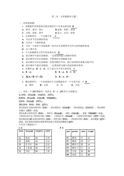
第二章 关系数据库习题二一、单项选择题:1、系数据库管理系统应能实现的专门关系运算包括 B 。
A .排序、索引、统计 B.选择、投影、连接 C .关联、更新、排序 D.显示、打印、制表2、关系模型中,一个关键字是 C 。
A .可由多个任意属性组成 B .至多由一个属性组成C .可由一个或多个其值能惟一标识该关系模型中任何元组的属性组成D .以上都不是3、个关系数据库文件中的各条记录 B 。
A .前后顺序不能任意颠倒,一定要按照输入的顺序排列B .前后顺序可以任意颠倒,不影响库中的数据关系C .前后顺序可以任意颠倒,但排列顺序不同,统计处理的结果就可能不同D .前后顺序不能任意颠倒,一定要按照关键字段值的顺序排列 4、有属性A ,B ,C ,D ,以下表示中不是关系的是 C 。
A .R (A ) B .R (A ,B ,C ,D ) C .D)C B R(A ⨯⨯⨯ D .R (A ,B )5、概念模型中,一个实体相对于关系数据库中一个关系中的一个 B 。
A 、属性 B 、元组 C 、列 D 、字段二、设有一个SPJ 数据库,包括S ,P ,J ,SPJ 四个关系模式: S( SNO ,SNAME ,STA TUS ,CITY); P(PNO ,PNAME ,COLOR ,WEIGHT); J(JNO ,JNAME ,CITY);SPJ(SNO ,PNO ,JNO ,QTY);供应商表S 由供应商代码(SNO )、供应商姓名(SNAME )、供应商状态(STATUS )、供应商所在城市(CITY )组成;零件表P 由零件代码(PNO )、零件名(PNAME )、颜色(COLOR )、重量(WEIGHT )组成; 工程项目表J 由工程项目代码(JNO )、工程项目名(JNAME )、工程项目所在城市(CITY )组成; 供应情况表SPJ 由供应商代码(SNO )、零件代码(PNO )、工程项目代码(JNO )、供应数量(QTY )组成,表示某供应商供应某种零件给某工程项目的数量为QTY 。
数据库系统教程习题答案(施伯乐)(第2版)_数据库原理和应用
第2部分各章习题解答及自测题第1章数据库概论1.1 基本内容分析1.1.1 本章的重要概念(1)DB、DBMS和DBS的定义(2)数据管理技术的发展阶段人工管理阶段、文件系统阶段、数据库系统阶段和高级数据库技术阶段等各阶段的特点。
(3)数据描述概念设计、逻辑设计和物理设计等各阶段中数据描述的术语,概念设计中实体间二元联系的描述(1:1,1:N,M:N)。
(4)数据模型数据模型的定义,两类数据模型,逻辑模型的形式定义,ER模型,层次模型、网状模型、关系模型和面向对象模型的数据结构以及联系的实现方式。
(5)DB的体系结构三级结构,两级映像,两级数据独立性,体系结构各个层次中记录的联系。
(6)DBMSDBMS的工作模式、主要功能和模块组成。
(7)DBSDBS的组成,DBA,DBS的全局结构,DBS结构的分类。
(1)教材P23的图1.24(四种逻辑数据模型的比较)。
(2)教材P25的图1.27(DB的体系结构)。
(3)教材P28的图1.29(DBMS的工作模式)。
(4)教材P33的图1.31(DBS的全局结构)。
1.2 教材中习题1的解答1.1 名词解释·逻辑数据:指程序员或用户用以操作的数据形式。
·物理数据:指存储设备上存储的数据。
·联系的元数:与一个联系有关的实体集个数,称为联系的元数。
·1:1联系:如果实体集E1中每个实体至多和实体集E2中的一个实体有联系,反之亦然,那么E1和E2的联系称为“1:1联系”。
·1:N联系:如果实体集E1中每个实体可以与实体集E2中任意个(零个或多个)实体有联系,而E2中每个实体至多和E1中一个实体有联系,那么E1和E2的联系是“1:N联系”。
·M:N联系:如果实体集E1中每个实体可以与实体集E2中任意个(零个或多个)实体有联系,反之亦然,那么E1和E2的联系称为“M:N联系”。
·数据模型:能表示实体类型及实体间联系的模型称为“数据模型”。
- 1、下载文档前请自行甄别文档内容的完整性,平台不提供额外的编辑、内容补充、找答案等附加服务。
- 2、"仅部分预览"的文档,不可在线预览部分如存在完整性等问题,可反馈申请退款(可完整预览的文档不适用该条件!)。
- 3、如文档侵犯您的权益,请联系客服反馈,我们会尽快为您处理(人工客服工作时间:9:00-18:30)。
第二章习题3
3. 定义并理解下列术语,说明它们之间的联系与区别:
( 1)域,关系,元组,属性
答:域:域是一组具有相同数据类型的值的集合。
关系:在域 D1,D2,…,Dn上笛卡尔积D1×D2×…×Dn的子集称为关系,表示为R(D1,D2,…,Dn)
元组:关系中的每个元素是关系中的元组。
属性:关系也是一个二维表,表的每行对应一个元组,表的每列对应一个域。
由于域可以相同,为了加以区分,必须对每列起一个名字,称为属性( Attribute)。
( 2)主码,候选码,外部码
答:候选码:若关系中的某一属性组的值能唯一地标识一个元组,则称该属性组为候选码( Candidate key)。
主码:若一个关系有多个候选码,则选定其中一个为主码( Primary key)。
外部码:设 F是基本关系R的一个或一组属性,但不是关系R的码,如果F与基本关系S 的主码Ks相对应,则称F是基本关系R的外部码(Foreign key),简称外码。
基本关系 R称为参照关系(Referencing relation),基本关系S称为被参照关系(Referenced relation)或目标关系(Target relation)。
关系R和S可以是相同的关系。
(3)关系模式,关系,关系数据库
关系模式:关系的描述称为关系模式( Relation Schema)。
它可以形式化地表示为: R (U,D,dom,F)
其中 R为关系名,U为组成该关系的属性名集合,D为属性组U中属性所来自的域,dom 为属性向域的映象集合,F为属性间数据的依赖关系集合。
关系:在域 D1,D2,…,Dn上笛卡尔积D1×D2×…×Dn的子集称为关系,表示为R(D1,D2,…,Dn)
关系是关系模式在某一时刻的状态或内容。
关系模式是静态的、稳定的,而关系是动态的、随时间不断变化的,因为关系操作在不断地更新着数据库中的数据。
关系数据库:关系数据库也有型和值之分。
关系数据库的型也称为关系数据库模式,是对关系数据库的描述,它包括若干域的定义以及在这些域上定义的若干关系模式。
关系数据库的值是这些关系模式在某一时刻对应的关系的集合,通常就称为关系数据库。
第二章习题5 用关系代数查询
(1) πSNO(σJNO=‘j1'(SPJ))
(2) πSNO(σJNO=‘j1‘∧PNO=‘p1’(SPJ))
(πSNO,PNO(σJNO=‘j1’(SPJ))πPNO(σCOLOR=‘红'(
(3) π
p)))
(4) πJNO(J)-πJNO(πSNO(σCITY=‘天津’(S))
π
(SPJ)
π
(σCOLOR=‘红'(p)))
(5) πPNO,JNO (SPJ) ÷πPNO(σSNO=‘S1'(SPJ))
第二章习题5 用ALPHA语言查询
(1)GET W (SPJ.SNO): SPJ.JNO=‘j1’
(2)GET W (SPJ.SNO): SPJ.JNO=‘j1’ ∧SPJ.PNO=‘p1’
(3)RANGE P PX
GET W (SPJ.SNO): ∃PX( PX.PNO=SPJ.PNO∧
SPJ.JNO=‘j1’ ∧PX.COLOR=‘红’)
(4)RANGE SPJ SPJX
P PX
S SX
GET W (SPJ.SNO): ∃SPJX ( SPJX.JNO=J.JNO∧
∃SX ( SX.SNO=SPJX.SNO∧SX.CITY=‘天津’ )∧
∃PX ( PX.PNO=SPJX.PNO∧PX.COLOR=‘红’))
(5) RANGE SPJ SPJX
SPJ SPJY
P PX
GET W(J.JNO): PX(∃SPJX
(SPJX.PNO=PX.PNO'∧SPJX.SNO=‘s1’)
∃SPJY(SPJY.JNO=J.JNO∧SPJY.PNO= PX.PNO)) 第二章习题6
自然连接与等值连接的区别:
(1) 自然连接有相同的属性列,等值连接相等分离不一定是相同属性列;
(2) 自然连接要消去公共属性列,等值连接不消去相同属性列。
自然连接与等值连接的联系:
(1) 自然连接和等值连接都是从笛卡尔积中选取满足条件的元组;
(2) 自然连接一定是等值连接,反之不成立。