Silhouette-Based Method for Object Classification and Human Action Recognition in Video

合集下载

A Discriminatively Trained, Multiscale, Deformable Part Model

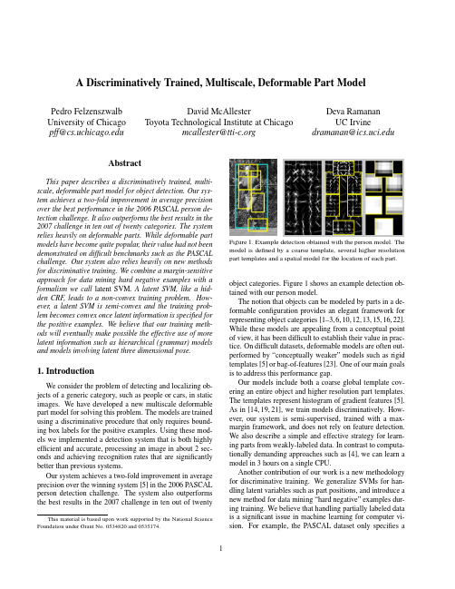
A Discriminatively Trained,Multiscale,Deformable Part ModelPedro Felzenszwalb University of Chicago pff@David McAllesterToyota Technological Institute at Chicagomcallester@Deva RamananUC Irvinedramanan@AbstractThis paper describes a discriminatively trained,multi-scale,deformable part model for object detection.Our sys-tem achieves a two-fold improvement in average precision over the best performance in the2006PASCAL person de-tection challenge.It also outperforms the best results in the 2007challenge in ten out of twenty categories.The system relies heavily on deformable parts.While deformable part models have become quite popular,their value had not been demonstrated on difﬁcult benchmarks such as the PASCAL challenge.Our system also relies heavily on new methods for discriminative training.We combine a margin-sensitive approach for data mining hard negative examples with a formalism we call latent SVM.A latent SVM,like a hid-den CRF,leads to a non-convex training problem.How-ever,a latent SVM is semi-convex and the training prob-lem becomes convex once latent information is speciﬁed for the positive examples.We believe that our training meth-ods will eventually make possible the effective use of more latent information such as hierarchical(grammar)models and models involving latent three dimensional pose.1.IntroductionWe consider the problem of detecting and localizing ob-jects of a generic category,such as people or cars,in static images.We have developed a new multiscale deformable part model for solving this problem.The models are trained using a discriminative procedure that only requires bound-ing box labels for the positive ing these mod-els we implemented a detection system that is both highly efﬁcient and accurate,processing an image in about2sec-onds and achieving recognition rates that are signiﬁcantly better than previous systems.Our system achieves a two-fold improvement in average precision over the winning system[5]in the2006PASCAL person detection challenge.The system also outperforms the best results in the2007challenge in ten out of twenty This material is based upon work supported by the National Science Foundation under Grant No.0534820and0535174.Figure1.Example detection obtained with the person model.The model is deﬁned by a coarse template,several higher resolution part templates and a spatial model for the location of each part. object categories.Figure1shows an example detection ob-tained with our person model.The notion that objects can be modeled by parts in a de-formable conﬁguration provides an elegant framework for representing object categories[1–3,6,10,12,13,15,16,22]. While these models are appealing from a conceptual point of view,it has been difﬁcult to establish their value in prac-tice.On difﬁcult datasets,deformable models are often out-performed by“conceptually weaker”models such as rigid templates[5]or bag-of-features[23].One of our main goals is to address this performance gap.Our models include both a coarse global template cov-ering an entire object and higher resolution part templates. The templates represent histogram of gradient features[5]. As in[14,19,21],we train models discriminatively.How-ever,our system is semi-supervised,trained with a max-margin framework,and does not rely on feature detection. We also describe a simple and effective strategy for learn-ing parts from weakly-labeled data.In contrast to computa-tionally demanding approaches such as[4],we can learn a model in3hours on a single CPU.Another contribution of our work is a new methodology for discriminative training.We generalize SVMs for han-dling latent variables such as part positions,and introduce a new method for data mining“hard negative”examples dur-ing training.We believe that handling partially labeled data is a signiﬁcant issue in machine learning for computer vi-sion.For example,the PASCAL dataset only speciﬁes abounding box for each positive example of an object.We treat the position of each object part as a latent variable.We also treat the exact location of the object as a latent vari-able,requiring only that our classiﬁer select a window that has large overlap with the labeled bounding box.A latent SVM,like a hidden CRF[19],leads to a non-convex training problem.However,unlike a hidden CRF, a latent SVM is semi-convex and the training problem be-comes convex once latent information is speciﬁed for thepositive training examples.This leads to a general coordi-nate descent algorithm for latent SVMs.System Overview Our system uses a scanning window approach.A model for an object consists of a global“root”ﬁlter and several part models.Each part model speciﬁes a spatial model and a partﬁlter.The spatial model deﬁnes a set of allowed placements for a part relative to a detection window,and a deformation cost for each placement.The score of a detection window is the score of the root ﬁlter on the window plus the sum over parts,of the maxi-mum over placements of that part,of the partﬁlter score on the resulting subwindow minus the deformation cost.This is similar to classical part-based models[10,13].Both root and partﬁlters are scored by computing the dot product be-tween a set of weights and histogram of gradient(HOG) features within a window.The rootﬁlter is equivalent to a Dalal-Triggs model[5].The features for the partﬁlters are computed at twice the spatial resolution of the rootﬁlter. Our model is deﬁned at aﬁxed scale,and we detect objects by searching over an image pyramid.In training we are given a set of images annotated with bounding boxes around each instance of an object.We re-duce the detection problem to a binary classiﬁcation prob-lem.Each example x is scored by a function of the form, fβ(x)=max zβ·Φ(x,z).Hereβis a vector of model pa-rameters and z are latent values(e.g.the part placements). To learn a model we deﬁne a generalization of SVMs that we call latent variable SVM(LSVM).An important prop-erty of LSVMs is that the training problem becomes convex if weﬁx the latent values for positive examples.This can be used in a coordinate descent algorithm.In practice we iteratively apply classical SVM training to triples( x1,z1,y1 ,..., x n,z n,y n )where z i is selected to be the best scoring latent label for x i under the model learned in the previous iteration.An initial rootﬁlter is generated from the bounding boxes in the PASCAL dataset. The parts are initialized from this rootﬁlter.2.ModelThe underlying building blocks for our models are the Histogram of Oriented Gradient(HOG)features from[5]. We represent HOG features at two different scales.Coarse features are captured by a rigid template covering anentireImage pyramidFigure2.The HOG feature pyramid and an object hypothesis de-ﬁned in terms of a placement of the rootﬁlter(near the top of the pyramid)and the partﬁlters(near the bottom of the pyramid). detection window.Finer scale features are captured by part templates that can be moved with respect to the detection window.The spatial model for the part locations is equiv-alent to a star graph or1-fan[3]where the coarse template serves as a reference position.2.1.HOG RepresentationWe follow the construction in[5]to deﬁne a dense repre-sentation of an image at a particular resolution.The image isﬁrst divided into8x8non-overlapping pixel regions,or cells.For each cell we accumulate a1D histogram of gra-dient orientations over pixels in that cell.These histograms capture local shape properties but are also somewhat invari-ant to small deformations.The gradient at each pixel is discretized into one of nine orientation bins,and each pixel“votes”for the orientation of its gradient,with a strength that depends on the gradient magnitude.For color images,we compute the gradient of each color channel and pick the channel with highest gradi-ent magnitude at each pixel.Finally,the histogram of each cell is normalized with respect to the gradient energy in a neighborhood around it.We look at the four2×2blocks of cells that contain a particular cell and normalize the his-togram of the given cell with respect to the total energy in each of these blocks.This leads to a vector of length9×4 representing the local gradient information inside a cell.We deﬁne a HOG feature pyramid by computing HOG features of each level of a standard image pyramid(see Fig-ure2).Features at the top of this pyramid capture coarse gradients histogrammed over fairly large areas of the input image while features at the bottom of the pyramid capture ﬁner gradients histogrammed over small areas.2.2.FiltersFilters are rectangular templates specifying weights for subwindows of a HOG pyramid.A w by hﬁlter F is a vector with w×h×9×4weights.The score of aﬁlter is deﬁned by taking the dot product of the weight vector and the features in a w×h subwindow of a HOG pyramid.The system in[5]uses a singleﬁlter to deﬁne an object model.That system detects objects from a particular class by scoring every w×h subwindow of a HOG pyramid and thresholding the scores.Let H be a HOG pyramid and p=(x,y,l)be a cell in the l-th level of the pyramid.Letφ(H,p,w,h)denote the vector obtained by concatenating the HOG features in the w×h subwindow of H with top-left corner at p.The score of F on this detection window is F·φ(H,p,w,h).Below we useφ(H,p)to denoteφ(H,p,w,h)when the dimensions are clear from context.2.3.Deformable PartsHere we consider models deﬁned by a coarse rootﬁlter that covers the entire object and higher resolution partﬁlters covering smaller parts of the object.Figure2illustrates a placement of such a model in a HOG pyramid.The rootﬁl-ter location deﬁnes the detection window(the pixels inside the cells covered by theﬁlter).The partﬁlters are placed several levels down in the pyramid,so the HOG cells at that level have half the size of cells in the rootﬁlter level.We have found that using higher resolution features for deﬁning partﬁlters is essential for obtaining high recogni-tion performance.With this approach the partﬁlters repre-sentﬁner resolution edges that are localized to greater ac-curacy when compared to the edges represented in the root ﬁlter.For example,consider building a model for a face. The rootﬁlter could capture coarse resolution edges such as the face boundary while the partﬁlters could capture details such as eyes,nose and mouth.The model for an object with n parts is formally deﬁned by a rootﬁlter F0and a set of part models(P1,...,P n) where P i=(F i,v i,s i,a i,b i).Here F i is aﬁlter for the i-th part,v i is a two-dimensional vector specifying the center for a box of possible positions for part i relative to the root po-sition,s i gives the size of this box,while a i and b i are two-dimensional vectors specifying coefﬁcients of a quadratic function measuring a score for each possible placement of the i-th part.Figure1illustrates a person model.A placement of a model in a HOG pyramid is given by z=(p0,...,p n),where p i=(x i,y i,l i)is the location of the rootﬁlter when i=0and the location of the i-th part when i>0.We assume the level of each part is such that a HOG cell at that level has half the size of a HOG cell at the root level.The score of a placement is given by the scores of eachﬁlter(the data term)plus a score of the placement of each part relative to the root(the spatial term), ni=0F i·φ(H,p i)+ni=1a i·(˜x i,˜y i)+b i·(˜x2i,˜y2i),(1)where(˜x i,˜y i)=((x i,y i)−2(x,y)+v i)/s i gives the lo-cation of the i-th part relative to the root location.Both˜x i and˜y i should be between−1and1.There is a large(exponential)number of placements for a model in a HOG pyramid.We use dynamic programming and distance transforms techniques[9,10]to compute the best location for the parts of a model as a function of the root location.This takes O(nk)time,where n is the number of parts in the model and k is the number of cells in the HOG pyramid.To detect objects in an image we score root locations according to the best possible placement of the parts and threshold this score.The score of a placement z can be expressed in terms of the dot product,β·ψ(H,z),between a vector of model parametersβand a vectorψ(H,z),β=(F0,...,F n,a1,b1...,a n,b n).ψ(H,z)=(φ(H,p0),φ(H,p1),...φ(H,p n),˜x1,˜y1,˜x21,˜y21,...,˜x n,˜y n,˜x2n,˜y2n,). We use this representation for learning the model parame-ters as it makes a connection between our deformable mod-els and linear classiﬁers.On interesting aspect of the spatial models deﬁned here is that we allow for the coefﬁcients(a i,b i)to be negative. This is more general than the quadratic“spring”cost that has been used in previous work.3.LearningThe PASCAL training data consists of a large set of im-ages with bounding boxes around each instance of an ob-ject.We reduce the problem of learning a deformable part model with this data to a binary classiﬁcation problem.Let D=( x1,y1 ,..., x n,y n )be a set of labeled exam-ples where y i∈{−1,1}and x i speciﬁes a HOG pyramid, H(x i),together with a range,Z(x i),of valid placements for the root and partﬁlters.We construct a positive exam-ple from each bounding box in the training set.For these ex-amples we deﬁne Z(x i)so the rootﬁlter must be placed to overlap the bounding box by at least50%.Negative exam-ples come from images that do not contain the target object. Each placement of the rootﬁlter in such an image yields a negative training example.Note that for the positive examples we treat both the part locations and the exact location of the rootﬁlter as latent variables.We have found that allowing uncertainty in the root location during training signiﬁcantly improves the per-formance of the system(see Section4).tent SVMsA latent SVM is deﬁned as follows.We assume that each example x is scored by a function of the form,fβ(x)=maxz∈Z(x)β·Φ(x,z),(2)whereβis a vector of model parameters and z is a set of latent values.For our deformable models we deﬁne Φ(x,z)=ψ(H(x),z)so thatβ·Φ(x,z)is the score of placing the model according to z.In analogy to classical SVMs we would like to trainβfrom labeled examples D=( x1,y1 ,..., x n,y n )by optimizing the following objective function,β∗(D)=argminβλ||β||2+ni=1max(0,1−y i fβ(x i)).(3)By restricting the latent domains Z(x i)to a single choice, fβbecomes linear inβ,and we obtain linear SVMs as a special case of latent tent SVMs are instances of the general class of energy-based models[18].3.2.Semi-ConvexityNote that fβ(x)as deﬁned in(2)is a maximum of func-tions each of which is linear inβ.Hence fβ(x)is convex inβ.This implies that the hinge loss max(0,1−y i fβ(x i)) is convex inβwhen y i=−1.That is,the loss function is convex inβfor negative examples.We call this property of the loss function semi-convexity.Consider an LSVM where the latent domains Z(x i)for the positive examples are restricted to a single choice.The loss due to each positive example is now bined with the semi-convexity property,(3)becomes convex inβ.If the labels for the positive examples are notﬁxed we can compute a local optimum of(3)using a coordinate de-scent algorithm:1.Holdingβﬁxed,optimize the latent values for the pos-itive examples z i=argmax z∈Z(xi )β·Φ(x,z).2.Holding{z i}ﬁxed for positive examples,optimizeβby solving the convex problem deﬁned above.It can be shown that both steps always improve or maintain the value of the objective function in(3).If both steps main-tain the value we have a strong local optimum of(3),in the sense that Step1searches over an exponentially large space of latent labels for positive examples while Step2simulta-neously searches over weight vectors and an exponentially large space of latent labels for negative examples.3.3.Data Mining Hard NegativesIn object detection the vast majority of training exam-ples are negative.This makes it infeasible to consider all negative examples at a time.Instead,it is common to con-struct training data consisting of the positive instances and “hard negative”instances,where the hard negatives are data mined from the very large set of possible negative examples.Here we describe a general method for data mining ex-amples for SVMs and latent SVMs.The method iteratively solves subproblems using only hard instances.The innova-tion of our approach is a theoretical guarantee that it leads to the exact solution of the training problem deﬁned using the complete training set.Our results require the use of a margin-sensitive deﬁnition of hard examples.The results described here apply both to classical SVMs and to the problem deﬁned by Step2of the coordinate de-scent algorithm for latent SVMs.We omit the proofs of the theorems due to lack of space.These results are related to working set methods[17].We deﬁne the hard instances of D relative toβas,M(β,D)={ x,y ∈D|yfβ(x)≤1}.(4)That is,M(β,D)are training examples that are incorrectly classiﬁed or near the margin of the classiﬁer deﬁned byβ. We can show thatβ∗(D)only depends on hard instances. Theorem1.Let C be a subset of the examples in D.If M(β∗(D),D)⊆C thenβ∗(C)=β∗(D).This implies that in principle we could train a model us-ing a small set of examples.However,this set is deﬁned in terms of the optimal modelβ∗(D).Given aﬁxedβwe can use M(β,D)to approximate M(β∗(D),D).This suggests an iterative algorithm where we repeatedly compute a model from the hard instances de-ﬁned by the model from the last iteration.This is further justiﬁed by the followingﬁxed-point theorem.Theorem2.Ifβ∗(M(β,D))=βthenβ=β∗(D).Let C be an initial“cache”of examples.In practice we can take the positive examples together with random nega-tive examples.Consider the following iterative algorithm: 1.Letβ:=β∗(C).2.Shrink C by letting C:=M(β,C).3.Grow C by adding examples from M(β,D)up to amemory limit L.Theorem3.If|C|<L after each iteration of Step2,the algorithm will converge toβ=β∗(D)inﬁnite time.3.4.Implementation detailsMany of the ideas discussed here are only approximately implemented in our current system.In practice,when train-ing a latent SVM we iteratively apply classical SVM train-ing to triples x1,z1,y1 ,..., x n,z n,y n where z i is se-lected to be the best scoring latent label for x i under themodel trained in the previous iteration.Each of these triples leads to an example Φ(x i,z i),y i for training a linear clas-siﬁer.This allows us to use a highly optimized SVM pack-age(SVMLight[17]).On a single CPU,the entire training process takes3to4hours per object class in the PASCAL datasets,including initialization of the parts.Root Filter Initialization:For each category,we auto-matically select the dimensions of the rootﬁlter by looking at statistics of the bounding boxes in the training data.1We train an initial rootﬁlter F0using an SVM with no latent variables.The positive examples are constructed from the unoccluded training examples(as labeled in the PASCAL data).These examples are anisotropically scaled to the size and aspect ratio of theﬁlter.We use random subwindows from negative images to generate negative examples.Root Filter Update:Given the initial rootﬁlter trained as above,for each bounding box in the training set weﬁnd the best-scoring placement for theﬁlter that signiﬁcantly overlaps with the bounding box.We do this using the orig-inal,un-scaled images.We retrain F0with the new positive set and the original random negative set,iterating twice.Part Initialization:We employ a simple heuristic to ini-tialize six parts from the rootﬁlter trained above.First,we select an area a such that6a equals80%of the area of the rootﬁlter.We greedily select the rectangular region of area a from the rootﬁlter that has the most positive energy.We zero out the weights in this region and repeat until six parts are selected.The partﬁlters are initialized from the rootﬁl-ter values in the subwindow selected for the part,butﬁlled in to handle the higher spatial resolution of the part.The initial deformation costs measure the squared norm of a dis-placement with a i=(0,0)and b i=−(1,1).Model Update:To update a model we construct new training data triples.For each positive bounding box in the training data,we apply the existing detector at all positions and scales with at least a50%overlap with the given bound-ing box.Among these we select the highest scoring place-ment as the positive example corresponding to this training bounding box(Figure3).Negative examples are selected byﬁnding high scoring detections in images not containing the target object.We add negative examples to a cache un-til we encounterﬁle size limits.A new model is trained by running SVMLight on the positive and negative examples, each labeled with part placements.We update the model10 times using the cache scheme described above.In each it-eration we keep the hard instances from the previous cache and add as many new hard instances as possible within the memory limit.Toward theﬁnal iterations,we are able to include all hard instances,M(β,D),in the cache.1We picked a simple heuristic by cross-validating over5object classes. We set the model aspect to be the most common(mode)aspect in the data. We set the model size to be the largest size not larger than80%of thedata.Figure3.The image on the left shows the optimization of the la-tent variables for a positive example.The dotted box is the bound-ing box label provided in the PASCAL training set.The large solid box shows the placement of the detection window while the smaller solid boxes show the placements of the parts.The image on the right shows a hard-negative example.4.ResultsWe evaluated our system using the PASCAL VOC2006 and2007comp3challenge datasets and protocol.We refer to[7,8]for details,but emphasize that both challenges are widely acknowledged as difﬁcult testbeds for object detec-tion.Each dataset contains several thousand images of real-world scenes.The datasets specify ground-truth bounding boxes for several object classes,and a detection is consid-ered correct when it overlaps more than50%with a ground-truth bounding box.One scores a system by the average precision(AP)of its precision-recall curve across a testset.Recent work in pedestrian detection has tended to report detection rates versus false positives per window,measured with cropped positive examples and negative images with-out objects of interest.These scores are tied to the reso-lution of the scanning window search and ignore effects of non-maximum suppression,making it difﬁcult to compare different systems.We believe the PASCAL scoring method gives a more reliable measure of performance.The2007challenge has20object categories.We entered a preliminary version of our system in the ofﬁcial competi-tion,and obtained the best score in6categories.Our current system obtains the highest score in10categories,and the second highest score in6categories.Table1summarizes the results.Our system performs well on rigid objects such as cars and sofas as well as highly deformable objects such as per-sons and horses.We also note that our system is successful when given a large or small amount of training data.There are roughly4700positive training examples in the person category but only250in the sofa category.Figure4shows some of the models we learned.Figure5shows some ex-ample detections.We evaluated different components of our system on the longer-established2006person dataset.The top AP scoreaero bike bird boat bottle bus car cat chair cow table dog horse mbike person plant sheep sofa train tvOur rank 31211224111422112141Our score .180.411.092.098.249.349.396.110.155.165.110.062.301.337.267.140.141.156.206.336Darmstadt .301INRIA Normal .092.246.012.002.068.197.265.018.097.039.017.016.225.153.121.093.002.102.157.242INRIA Plus.136.287.041.025.077.279.294.132.106.127.067.071.335.249.092.072.011.092.242.275IRISA .281.318.026.097.119.289.227.221.175.253MPI Center .060.110.028.031.000.164.172.208.002.044.049.141.198.170.091.004.091.034.237.051MPI ESSOL.152.157.098.016.001.186.120.240.007.061.098.162.034.208.117.002.046.147.110.054Oxford .262.409.393.432.375.334TKK .186.078.043.072.002.116.184.050.028.100.086.126.186.135.061.019.036.058.067.090Table 1.PASCAL VOC 2007results.Average precision scores of our system and other systems that entered the competition [7].Empty boxes indicate that a method was not tested in the corresponding class.The best score in each class is shown in bold.Our current system ranks ﬁrst in 10out of 20classes.A preliminary version of our system ranked ﬁrst in 6classes in the ofﬁcial competition.BottleCarBicycleSofaFigure 4.Some models learned from the PASCAL VOC 2007dataset.We show the total energy in each orientation of the HOG cells in the root and part ﬁlters,with the part ﬁlters placed at the center of the allowable displacements.We also show the spatial model for each part,where bright values represent “cheap”placements,and dark values represent “expensive”placements.in the PASCAL competition was .16,obtained using a rigid template model of HOG features [5].The best previous re-sult of.19adds a segmentation-based veriﬁcation step [20].Figure 6summarizes the performance of several models we trained.Our root-only model is equivalent to the model from [5]and it scores slightly higher at .18.Performance jumps to .24when the model is trained with a LSVM that selects a latent position and scale for each positive example.This suggests LSVMs are useful even for rigid templates because they allow for self-adjustment of the detection win-dow in the training examples.Adding deformable parts in-creases performance to .34AP —a factor of two above the best previous score.Finally,we trained a model with partsbut no root ﬁlter and obtained .29AP.This illustrates the advantage of using a multiscale representation.We also investigated the effect of the spatial model and allowable deformations on the 2006person dataset.Recall that s i is the allowable displacement of a part,measured in HOG cells.We trained a rigid model with high-resolution parts by setting s i to 0.This model outperforms the root-only system by .27to .24.If we increase the amount of allowable displacements without using a deformation cost,we start to approach a bag-of-features.Performance peaks at s i =1,suggesting it is useful to constrain the part dis-placements.The optimal strategy allows for larger displace-ments while using an explicit deformation cost.The follow-Figure 5.Some results from the PASCAL 2007dataset.Each row shows detections using a model for a speciﬁc class (Person,Bottle,Car,Sofa,Bicycle,Horse).The ﬁrst three columns show correct detections while the last column shows false positives.Our system is able to detect objects over a wide range of scales (such as the cars)and poses (such as the horses).The system can also detect partially occluded objects such as a person behind a bush.Note how the false detections are often quite reasonable,for example detecting a bus with the car model,a bicycle sign with the bicycle model,or a dog with the horse model.In general the part ﬁlters represent meaningful object parts that are well localized in each detection such as the head in the person model.Figure6.Evaluation of our system on the PASCAL VOC2006 person dataset.Root uses only a rootﬁlter and no latent place-ment of the detection windows on positive examples.Root+Latent uses a rootﬁlter with latent placement of the detection windows. Parts+Latent is a part-based system with latent detection windows but no rootﬁlter.Root+Parts+Latent includes both root and part ﬁlters,and latent placement of the detection windows.ing table shows AP as a function of freely allowable defor-mation in theﬁrst three columns.The last column gives the performance when using a quadratic deformation cost and an allowable displacement of2HOG cells.s i01232+quadratic costAP.27.33.31.31.345.DiscussionWe introduced a general framework for training SVMs with latent structure.We used it to build a recognition sys-tem based on multiscale,deformable models.Experimental results on difﬁcult benchmark data suggests our system is the current state-of-the-art in object detection.LSVMs allow for exploration of additional latent struc-ture for recognition.One can consider deeper part hierar-chies(parts with parts),mixture models(frontal vs.side cars),and three-dimensional pose.We would like to train and detect multiple classes together using a shared vocab-ulary of parts(perhaps visual words).We also plan to use A*search[11]to efﬁciently search over latent parameters during detection.References[1]Y.Amit and A.Trouve.POP:Patchwork of parts models forobject recognition.IJCV,75(2):267–282,November2007.[2]M.Burl,M.Weber,and P.Perona.A probabilistic approachto object recognition using local photometry and global ge-ometry.In ECCV,pages II:628–641,1998.[3] D.Crandall,P.Felzenszwalb,and D.Huttenlocher.Spatialpriors for part-based recognition using statistical models.In CVPR,pages10–17,2005.[4] D.Crandall and D.Huttenlocher.Weakly supervised learn-ing of part-based spatial models for visual object recognition.In ECCV,pages I:16–29,2006.[5]N.Dalal and B.Triggs.Histograms of oriented gradients forhuman detection.In CVPR,pages I:886–893,2005.[6] B.Epshtein and S.Ullman.Semantic hierarchies for recog-nizing objects and parts.In CVPR,2007.[7]M.Everingham,L.Van Gool,C.K.I.Williams,J.Winn,and A.Zisserman.The PASCAL Visual Object Classes Challenge2007(VOC2007)Results./challenges/VOC/voc2007/workshop.[8]M.Everingham, A.Zisserman, C.K.I.Williams,andL.Van Gool.The PASCAL Visual Object Classes Challenge2006(VOC2006)Results./challenges/VOC/voc2006/results.pdf.[9]P.Felzenszwalb and D.Huttenlocher.Distance transformsof sampled functions.Cornell Computing and Information Science Technical Report TR2004-1963,September2004.[10]P.Felzenszwalb and D.Huttenlocher.Pictorial structures forobject recognition.IJCV,61(1),2005.[11]P.Felzenszwalb and D.McAllester.The generalized A*ar-chitecture.JAIR,29:153–190,2007.[12]R.Fergus,P.Perona,and A.Zisserman.Object class recog-nition by unsupervised scale-invariant learning.In CVPR, 2003.[13]M.Fischler and R.Elschlager.The representation andmatching of pictorial structures.IEEE Transactions on Com-puter,22(1):67–92,January1973.[14] A.Holub and P.Perona.A discriminative framework formodelling object classes.In CVPR,pages I:664–671,2005.[15]S.Ioffe and D.Forsyth.Probabilistic methods forﬁndingpeople.IJCV,43(1):45–68,June2001.[16]Y.Jin and S.Geman.Context and hierarchy in a probabilisticimage model.In CVPR,pages II:2145–2152,2006.[17]T.Joachims.Making large-scale svm learning practical.InB.Sch¨o lkopf,C.Burges,and A.Smola,editors,Advances inKernel Methods-Support Vector Learning.MIT Press,1999.[18]Y.LeCun,S.Chopra,R.Hadsell,R.Marc’Aurelio,andF.Huang.A tutorial on energy-based learning.InG.Bakir,T.Hofman,B.Sch¨o lkopf,A.Smola,and B.Taskar,editors, Predicting Structured Data.MIT Press,2006.[19] A.Quattoni,S.Wang,L.Morency,M.Collins,and T.Dar-rell.Hidden conditional randomﬁelds.PAMI,29(10):1848–1852,October2007.[20] ing segmentation to verify object hypothe-ses.In CVPR,pages1–8,2007.[21] D.Ramanan and C.Sminchisescu.Training deformablemodels for localization.In CVPR,pages I:206–213,2006.[22]H.Schneiderman and T.Kanade.Object detection using thestatistics of parts.IJCV,56(3):151–177,February2004. [23]J.Zhang,M.Marszalek,zebnik,and C.Schmid.Localfeatures and kernels for classiﬁcation of texture and object categories:A comprehensive study.IJCV,73(2):213–238, June2007.。

HONORS AND AWARDS

July27,2007Marcus J.GroteProfessor of Numerical Analysis andComputational MathematicsDepartement Mathematik,Universit¨a t BaselRheinsprung21,CH–4051BaselEDUCATION1990–1995Stanford University,USAPh.D.in Scientiﬁc Computing and Computational Mathematics,graduated Spring95.Advisor:Professor Joseph B.Keller.Dissertation:”Nonreﬂecting Boundary Conditions”Ph.D.minor in Mathematics,Ph.D.minor in Mechanical Engineering.1985–1990Universit´e de Gen`e ve,Geneva,SwitzerlandDiplˆo me de math´e maticien,equivalent to an M.S.in Mathematics.Advisor:Professor Gerhard Wanner.1985–1990Universit´e de Gen`e ve,Geneva,SwitzerlandDiplˆo me d’informaticien,equivalent to an M.S.in Computer Science. PERSONAL DATASwiss citizen(GE),married,two childrenPlace and date of birth:G¨o ttingen,Germany,on December27,1966HONORS AND A W ARDSSpring2001Oﬀered the Chair of Numerical Analysis(C-4Professur)at the L.-M.-Universit¨a t M¨u nchen,Munich,Germany.Declined May2001.1993–1995IBM graduate fellowship,nationwide(USA)competitionAugust1992IMA,University of MinnesotaCompetitive admission to a four week workshop on mathematical modeling in en-gineering science and industry1990–1991Graduate fellowship,School of Engineering,Stanford University PROFESSIONAL APPOINTMENTS2001–present Department of Mathematics,Universit¨a t Basel,Basel,Switzerland Professor of Numerical analysis and computational mathematics.2004–2005Courant Institute,NYU,New York,USAVisiting professor,on sabbatical leave.1997–2001Department of Mathematics,ETH,Z¨u rich,SwitzerlandAssistant professor.1995–1997Courant Institute of Mathematical Sciences,New YorkAssociate research scientist.Post-doctoral position under Prof.Andrew Majda. Summer1993U.C.San Francisco,San Francisco,CaliforniaResearch assistant.Collaborated with Prof.David A.Agard,Department of Bio-chemistry.Implemented a complete volume rendering algorithm for the display andanalysis of three-dimensional biological images coming from confocal microscopy.1Summer1992NASA Ames,Moﬀett Field,CaliforniaResearch assistant.Continued the work started in summer1991with Dr.HorstSimon on the Connection Machine CM–bined the preconditioner with aniterative solver,and applied the method to an extensive set of test problems comingfrom scientiﬁc and industrial applications.Summer1991NASA Ames,Moﬀett Field,CaliforniaResearch assistant.Collaborated with Dr.Horst Simon.Implemented a parallelpreconditioner for the iterative solution of large linear systems on the ConnectionMachine CM–2.INVITED TALKSJun.2008FoCM2008conference,Hong-Kong,on DG-FEM and local time-steppingNov.2007BIRS,Banﬀ,Canada,meeting on DG-FEMNov.2007Universit´e Louis Pasteur,Strasbourg,on DG-FEM and local time-steppingApr.2007Lawrence Livermore b.,USA,on DG-FEM and local time-steppingMar.2007Stanford50conference,USA,on Multiple scattering and DG-FEMMar.2007Universit¨a t Innsbruck,Austria,on DG-FEM and local time steppingFeb.2007Oberwolfach,Germany,meeting on Computational Electromagnetics and Acoustics Nov.2006INRIA,Rocquencourt,France,winter school“Ecole des Ondes”on DG-FEM Aug.2006Oberwolfach,Germany,meeting on Math.Th.and Model.in Atm.-Ocean Science May2006Universit¨a t Z¨u rich,Switzerland,on Multiple scattering and DG-FEMMar.2006Universit´e de Gen`e ve,Switzerland,on Multiple scattering and DG-FEMJan.2006Universit´e de Fribourg,Switzerland,on Multiple scattering and DG-FEMNov.2005Universit¨a t Karslruhe,Germany,on Multiple scattering and DG-FEMNov.2005Techn.Universit¨a t M¨u nchen,Germany,on Multiple scattering and DG-FEM Mar.2005University of Delaware,USA,on Multiple scatteringMar.2005NJIT,USA,on Multiple scatteringMar.2005Stanford University,USA,on Multiple scatteringFeb.2005Courant Institute,USA,on Multiple scatteringFeb.2005Columbia University,USA,on Multiple scatteringJul.2004WIAS Berlin,Germany,Nonreﬂecting boundary conditionsFeb.2004Oberwolfach,Germany,meeting on Computational ElectromagneticsMay2003Universit¨a t M¨u nster,Germany,on Wave propagation in unbounded mediaDec.2002Universit´e de Haute-Alsace,Mulhouse,France,on Wave prop.in unbound.med. Aug.2002Oberwolfach,Germany,meeting on Math.Th.and Model.in Atm.-Ocean Science Mar.2002HYP2002conference,Caltech,CA,on Nonreﬂecting boundary conditionsJuly2001Universit¨a t Freiburg i.Br.,Germany,on Nonreﬂecting boundary conditions Jan.2001RWTH Aachen,Germany,on Parallel preconditioning with approximate inverses Aug.2000PMAA2000meeting,Switzerland,tutorial on the SPAI AlgorithmJune2000Universit¨a t Heidelberg,Germany,on Nonreﬂecting boundary conditionsMar.2000Universit´e de Rennes,France,on Modeling geophysicalﬂows via statistical theory Feb.2000EPFL,Switzerland,on Nonreﬂecting boundary conditions2Dec.1999L.-M.-Universit¨a t M¨u nchen,Germany,on Nonreﬂecting boundary conditions Dec.1999Universit¨a t Z¨u rich,Switzerland,on Nonreﬂecting boundary conditionsDec.1999Universit¨a t Basel,Switzerland,on Nonreﬂecting boundary conditionsJune1999Oberwolfach,Germany,meeting on Fast Solvers for PDE’sFeb.1999Techn.Universit¨a t M¨u nchen,Germany,on Nonreﬂecting boundary conditions Jan.1999Universit´e de Fribourg,Switzerland,on Nonreﬂecting boundary conditionsJune1998ETH Z¨u rich,Switzerland,on Modeling large scale geophysicalﬂowsJune1998Oxford University,UK,on Nonreﬂecting boundary conditionsJune1998Oxford University,UK,on Parallel preconditioningMay1998Universit¨a t T¨u bingen,Germany,on Nonreﬂecting boundary conditionsDec.1997Courant Institute,NY,on Large and small scale interaction via topographic stress Nov.1997Universit¨a t G¨o ttingen,Germany,on Nonreﬂecting boundary conditionsMarch1997ETH,Z¨u rich,Switzerland,on Nonreﬂecting boundary conditionsApril1996University of Maryland,MD,on Nonreﬂecting boundary conditionsFeb.1996NJIT,Institute of Technology,NJ,on Nonreﬂecting boundary conditionsNov.1995AT&T,Bell Labs,NJ,on Nonreﬂecting boundary conditionsNov.1995Courant Institute,NY,on Nonreﬂecting boundary conditionsAug.1995Swiss Center for Supercomputing(CSCS),on Parallel preconditioning3TEACHING EXPERIENCEFall2001–Universit¨a t BaselSince Fall2001,teaching undergraduate and graduate level courses in Linear Alge-bra,Numerical Analysis,Applied Analysis,etc.Responsible for a“Mathematics laboratory”course at the computer on the use ofMaple,Matlab,LaTex,C.THESES DIRECTEDFall2005–I.Sim,Local nonreﬂecting boundary conditions for multiple scattering,Ph.D.thesis (Dept.of Mathematics,Uni Basel),ongoing work.Fall2003–V.Palumberi,Mathematical modeling and simulation of cell populations,Ph.D.thesis(Dept.of Mathematics,Uni Basel),ongoing work.July2006 A.Schneebeli,Interior Penalty Discontinuous Galerkin Methods for Electromag-netic and Acoustic Wave Equations,Ph.D.thesis(Dept.of Mathematics,UniBasel).April2005 C.Kirsch,Nonreﬂecting boundary conditions for the numerical solution of wave propagation problems in unbounded domains,Ph.D.thesis(Dept.of Mathematics,Uni Basel).June2004J.Mittmann,Preconditioning symmetric indeﬁnite linear systems with factorized sparse approximate inverses,Ms.thesis(Dept.of Mathematics).Together withDr.Olaf Schenk.June2003P.Meury,Existence and Uniqueness in DtN Maps for Multiple Scattering,Ms.thesis(Dept.of Mathematics).March2003U.Hasler,Mixed Finite Element Approximation of an Incompressible MHD Problem based on Weighted Regularization,Ms.thesis(Dept.of Mathematics).Togetherwith Prof.D.Sch¨o tzau.May2003O.Br¨o ker,Parallel Multigrid Methods using Sparse Approximate Inverses,Ph.D.thesis(Dept.of Computer Science,ETH Z¨u rich).Sept.2000G.G¨a chter,Nonreﬂecting Boundary Conditions for Three-dimensional Elastic Waves, Ms.thesis(Dept.of Mathematics).March2001 D.Hoch,High-order Finite Element Method for Time-dependent Scattering in Com-plex Geometry,Ms.thesis(Computational Sciences and Engineering Program). March2001 C.Hohenegger,Variational Formulation and Energy Estimates for Nonreﬂecting Boundary Conditions,Ms.thesis(Dept.of Mathematics).March2001 C.Kirsch,Sparse Approximate Inverse Smoothers,Ms.thesis(Dept.of Mathemat-ics).NUMERICAL SOFTW AREJune1994SPAI,SParse Approximate Inverse preconditioner,fortran77version,joint work with Prof.T.Huckle,TU-M¨u nchen,see ftp:///pub/grote/spai/May1999SPAI Version3.0,C/MPI parallel version,PETSc interface,Matlab interface,joint work with S.Barnard,NASA Ames Research Center,see http://www.sam.math.ethz.ch/˜grote/spai/Mar.2006SPAI Version3.2,auto conﬁgure installation andﬁxed sparsity added,new Matlab functions spaidiags,spaitau added,joint work with O.Br¨o ker and M.Hage-mann,see putational.unibas.ch/software/spai/4SPECIAL SKILLSBilingual in French and German,ﬂuent in English.Experienced in Fortran,C,Unix,L A T E X,Matlab,and Mathematica.Parallel programming experience on the Connection Machine CM–2,on the SGI/CraySV–1,and on the NEC SX–4.PROFESSIONAL ACTIVITIESJuly2007ICIAM07,Internat.Congress on Industrial and Applied Mathematics,Zurich, Switzerland,member of the scientiﬁc committee.June2004CANUM04,Congr`e s National d’Analyse Num´e rique,Obernai,France,member of the scientiﬁc committee.June2003BASNUM03,Spring Meeting of the Swiss Mathematical Society,organisor(withD.Sch¨o tzau).Nov.2002PMAA2002,Neuchˆa tel,SwitzerlandMember of the organizing committee.Minisymposium on Parallel Algebraic Multigrid Methods(with O.Schenk)July2001AMCW01,Berlin,GermanyOrganized two minisymposia:Statistical mechanics models for the atmosphere and ocean(with.A.Majda);Numerical methods for wave propagation in unbounded media(with F.Schmidt) Feb.2001GAMM2001,ETH Z¨u rich,member of the organizing committeeAug.2000PMAA2000,Neuchˆa tel,SwitzerlandOrganized a minisymposium on Sparse approximate inverses at the Internationalworkshop on parallel matrix algorithms and applications(with P.Arbenz,ETHZ) July1999ENUMATH99,Jyv¨a vskyl¨a,FinlandOrganized a minisymposium on Mathematical and numerical modeling in atmosphere-ocean science(with A.Majda)1997–2001Member of the committee responsible for inviting guests for post-graduate lectures at the ETH Z¨u rich1997–present Acting referee for SIAM Journal on Scientiﬁc Computing,SIAM Journal on Ap-plied Mathematics,SIAM Journal on Numerical Analysis,SIAM Journal on MatrixAnalysis,Journal of Computational Physics,Numerische Mathematik,Journal ofthe Acoustical Society of America,Computer Methods in Applied Mechanics and En-gineering,European Journal of Applied Mathematics,Mathematics and Computersin Simulation,High Performance Computing Applications,ZAMPREFERENCESAvailable upon request from:Prof.Gene H.Golub,Dept.of Computer Science,Stanford University,Stanford,CA94305,(415)723–3124.Prof.Joseph B.Keller,Depts.of Mathematics and Mechanical Engineering,Stan-ford University,Stanford,CA94305,(415)723–0851.Prof.Andrew J.Majda,Courant Institute of Mathematical Sciences,251MercerSt.,New York,NY10012,(212)998–3323.Prof.Gerhard Wanner,D´e pt.de Math´e matiques,Universit´e de Gen`e ve,2–4ruedu Li`e vre,CH–1211Gen`e ve4,Switzerland,(+41)22702–6952.5JOURNAL PUBLICATIONS•(with A.Schneebeli and D.Sch¨o tzau)Interior Penalty Discontinuous GalerkinMethod for Maxwell’s Equations:Optimal L2-Norm Error Estimates,IMA J.Nu-mer.Analysis,in press.•(with A.J.Majda)Explicit Oﬀ-line Test Criteria for Stable Accurate Time Filteringof Strongly Unstable Spatially Extended Systems,Proc.Natl.Acad.Sciences104,pp.1124–1129(2007).•(with C.Kirsch)Nonreﬂecting Boundary Conditions for Time Dependent MultipleScattering,p.Physics221,pp.41–62(2007).•(with A.Schneebeli and D.Sch¨o tzau)Interior Penalty Discontinuous GalerkinMethod for Maxwell’s Equations:Energy Norm Error Estimates,put.Appl.Math.204,pp.375–386(2007).•(with A.Schneebeli and D.Sch¨o tzau)Discontinuous Galerkin Finite Element MethodFor The Wave Equation,SIAM J.Num.Analysis,44,pp.2408–2431(2006).•(with A.J.Majda)Stable Time Filtering of Strongly Unstable Spatially ExtendedSystems,Proc.Natl.Acad.Sciences,103,pp.7548–7553(2006).•Local Nonreﬂecting Boundary Conditions for Maxwell’s Equations,Comput.Meth-ods Appl.Mech.Engrg.195,pp.3691–3708(2006).•(with A.Barbero,V.Palumberi,B.Wagner,et al.)Experimental and MathematicalStudy of the Inﬂuence of Growth Factors on the Growth Kinetics of Adult HumanArticular Chondrocytes,J.Cell.Physiology204,pp.830–838(2005).•(with C.Kirsch)Dirichlet-to-Neumann Boundary Conditions for Multiple Scatter-ing Problems,p.Phys.201,pp.630–650(2004).•(with W.Bangerth and C.Hohenegger)Finite Element Method for Time Depen-dent Scattering:Nonreﬂecting Boundary Conditions,Adaptivity,and Energy Decay,Comp.Meth.Appl.Mech.Engrg.193,pp.2453–2482(2004).•(with G.G¨a chter)Dirichlet-to-Neumann Map for Three-Dimensional Elastic Waves,Wave Motion,vol.37/3,pp.293–311(2003).•(with O.Br¨o ker)Sparse Approximate Inverse Smoothers For Geometric and Alge-braic Multigrid,Appl.Num.Math.41,pp.61–80(2002).•(with O.Br¨o ker,C.Mayer,and A.Reusken)Robust Parallel Smoothing for Multi-grid via Sparse Approximate Inverses,SIAM put.23,pp.1396–1417(2001).•(with M.T.DiBattista and A.J.Majda)Meta-stability of Equilibrium StatisticalStructures for Prototype Geophysical Flows with Damping and Driving,Physica D:151,271–304(2001).•Nonreﬂecting Boundary Condition for Elastodynamic Scattering,put.Phys.161,331–353(2000).•(with A.J.Majda)Crude Closure for Flow with Topography Through Large ScaleStatistical Theory,Nonlinearity13,569–600(2000).•Am Rande des Unendlichen–Numerische Verfahren f¨u r unbegrenzte Gebiete,(Nu-merical methods for unbounded domains,in German),Elem.Math.55,67–83(2000).•(with J.B.Keller)Exact Nonreﬂecting Boundary Condition for Elastic Waves,SIAMJ.Appl.Math.60,803–819(2000).6•Nonreﬂecting Boundary Conditions for Electromagnetic Scattering,Int.J.Numer.Model.13,397–416(2000).(Special issue on absorbing boundary conditions forcomputational electromagnetics).•(with A.J.Majda,and C.Ragazzo)Dynamic Mean Flow and Small-Scale Interac-tion Through Topographic Stress,J.Nonlin.Science9,89–130(1999).•(with J.B.Keller)Nonreﬂecting Boundary Conditions for Maxwell’s Equations,J.of Comput.Phys.139,327–342(1998).•(with A.J.Majda)Model Dynamics and Vertical Collapse in Decaying StronglyStratiﬁed Flows,Phys.of Fluids9,2932–2940(1997).•(with A.J.Majda)Crude Closure Dynamics Through Large Scale Statistical Theo-ries,Phys.of Fluids9,3431–3442(1997).•(with T.Huckle)Parallel Preconditioning with Sparse Approximate Inverses,SIAMJ.of put.18,838–853(1997).•(with J.B.Keller)Nonreﬂecting Boundary Conditions for Time Dependent Scatter-ing,J.of Comput.Phys.127,52–65(1996).•(with J.B.Keller)On Nonreﬂecting Boundary Conditions,J.of Comput.Phys.122,231–243(1995).•(with J.B.Keller)Exact Nonreﬂecting Boundary Conditions for the Time-dependentWave Equation,SIAM J.of Appl.Math.55,280–297(1995).REFEREED CONFERENCE PROCEEDINGS•(with I.Sim)Exact local nonreﬂecting boundary conditions for time-dependent mul-tiple scattering,in Proc.of6th Intern.Congress on Indust.and Appl.Math.(ICIAM2007),held in Zurich,July16–20,2007.•(with Ch.Kirsch)Nonreﬂecting boundary condition for time-dependent multiplescattering,in Etude de la propagation ultrasonore en milieux non-homog`e nes envue du contrˆo le non destructif(Proc.Journ´e es du GDR US,France,2006);Eds.M.Deschamps,B.Desoudin,A.L´e ger,INRIA,pp.210–218,2007.•(with J.Diaz)Explicit energy conserving local time stepping for second order waveequations,in Proc.of8th Intern.Conf.on Math.and Numerical Aspects of WavePropagation(WAVES2007),pp.263–265,held at Univ.of Reading,UK,July23–27,2007.•(with I.Sim)Local nonreﬂecting boundary conditions for time-dependent multiplescattering,in Proc.of8th Intern.Conf.on Math.and Numerical Aspects ofWave Propagation(WAVES2007),pp.283–285,held at Univ.of Reading,UK,July23–27,2007.•(with O.Schenk,M.Bollh¨o fer)Algebraic multilevel preconditioning for Helmholtzequation,in Proc.of Europ.Conf.on Comput.Fluid Dynamics(ECCOMAS CFD2006),held in Egmond aan Zee,The Netherlands,Sept.5–8,2006.•(with A.Schneebeli,D.Sch¨o tzau)Interior penalty DG-FEM for second order waveequations,in Proc.of7th Intern.Conf.on Math.and Numerical Aspects of WavePropagation(WAVES2005),pp.408–410,held at Brown Univ.,June20–24,2005.•(with C.Kirsch,P.Meury)Nonreﬂecting boundary conditions for multiple domainwave scattering in unbounded media,In Numerical Mathematics and Advanced Ap-plications(Proc.ENUMATH2003),M.Feistauer,V.Dolejˇs´ı,P.Knobloch,K.Najzar,eds.,Springer,2004,pp.391–3997•(with C.Kirsch)Dirichlet-to-Neumann boundary condition for multiple scatteringproblems,in Proc.of Sixth Intern.Conf.on Math.and Numerical Aspects of WavePropagation(WAVES2003),Eds.G.Cohen et al.,Springer-Vg,2003,pp.263–267.•(with C.Kirsch)Far-ﬁeld evaluation via nonreﬂecting boundary conditions,in Proc.of Ninth Intern.Conf.on Hyperbolic Problems:Theory,Numerics,Applications(HYP2002),Eds.T.Hou and E.Tadmor,Springer-Vg,2003,pp.195–201.•(with O.Br¨o ker)Parallel smoothing for multigrid with sparse approximate inverses,in Proc.of Third Intern.Conf.on High-Performance puting:Meth.,Developments,and Applic.(FORTWIHR2001),held in Erlangen,Germany,March2001.•(with O.Br¨o ker)Parallel Algebraic Multigrid via Sparse Approximate Inverses,inProc.of16th IMACS World Congress2000,held in Lausanne,Switzerland,August2000.•(with A.J.Majda,and M.G.Shefter)Analytical Models for Vertical Collapse andInstability in Strongly Stratiﬁed Flows,in Proceedings of IUTAM Conference onRotating Stratiﬁed Turbulence,(held in Boulder,Colorado,1998),edited by Kerr,Herring and Kimura,2000.•Nonreﬂecting Boundary Conditions for the Simulation of Elastic Waves in Un-bounded Media,in Proc.Fifth Internat.Conf.on Math.and Numerical Aspectsof Wave Propagation(WAVES2000),held in Santiago de Compostela,Spain,July2000.•(with A.J.Majda)Crude Closure Dynamics for Geophysical Flows via Large ScaleStatistical Theory,in Proc.of the12th Conf.on Atmospheric and Oceanic FluidDynamics,held in New York,NY,June1999.•(with S.Barnard)A Block Version of the SPAI Preconditioner,Proceedings of the9th SIAM conference on Parallel Processing for Scientiﬁc Computing,San Antonio,TX,March1999.•(with V.Deshpande,P.Messmer,and W.Sawyer)Parallel Implementation of aSparse Approximate Inverse Preconditioner,in Proceedings of Irregular’96,held inSanta Barbara,CA,August1996.•(with T.Huckle)Eﬀective Parallel Preconditioning with Sparse Approximate In-verses,Proceedings of the7th SIAM conference on Parallel Processing for ScientiﬁcComputing,San Francisco,CA,February1995.•(with J.B.Keller)Nonreﬂecting Boundary Conditions,Anniversary volume,DanishCenter for Applied Mathematics and Mechanics,Lyngby,Denmark,1994.•(with H.D.Simon)Parallel Preconditioning and Approximate Inverses on the Con-nection Machine,Proceedings of the6th SIAM conference on Parallel Processingfor Scientiﬁc Computing,Norfolk,VA,March1993.•(with H.D.Simon)Parallel Preconditioning and Approximate Inverses on the Con-nection Machine,Proceedings of the Scalable High Performance Computing Con-ference(SHPCC)1992,Williamsburg,VA,April1992,IEEE Comp.Sc.Press. BOOKS AND MONOGRAPHS•Local and Nonlocal Nonreﬂecting Boundary Conditions for Electromagnetic Scat-tering,in Modeling and Computations in Electromagnetics(Ed.H.Ammari),Lect.Notes in Comput.Sciences and Engin.,vol.59,Springer,2007.8•Information Theory and Stochastics for Multiscale Nonlinear Systems,A.J.Majda,R.V.Abramov,and M.J.Grote,Amer.Math.Soc.,Providence,USA,2005•Nonreﬂecting Boundary Conditions for Time Dependent Waves,in A Celebrationof Mathematical Modeling,The Joseph B.Keller Anniversary Volume(Eds. D.Givoli,M.J.Grote,G.Papanicolaou),Kluwer Acad.Publ.,2004.•Nonreﬂecting Boundary Conditions,in Absorbing Boundaries and Layers,DomainDecomposition Methods(Eds.L.Halpern,L.Tourrette),Nova Science Publishers,Inc.,New York,2001.•(with H.Chen,J.Swedlow,et al.)The Collection,Processing and Display of Dig-ital Three-Dimensional Images in Biological Specimens,in Handbook of BiologicalConfocal Microscopy,2nd ed.,ed.J.Pawley,Plenum,NY,1995.•(et al.)A model for venous bloodﬂow in the legs,Model of radionuclide contam-inants in an aquifer,Flame propagation through combustible gases in a cylinder,Flow improvement in hydrofractured reservoirs,in Mathematical Modeling,IMAPreprint Series#1021,University of Minnesota,1992.UNPUBLISHED ADDRESSES,ABSTRACTS,POSTERS,ETC.•(with A.Barbero,I.Martin,V.Palumberi,and B.Wagner)Spatio-angular modelingfor the formation of oriented patches in chondrocyte cultures,Biovalley Life SciencesWeek2007,held in Basel,Switzerland,Oct.19–23,2007.•(with J.Diaz)Energy conserving explicit local time stepping for second order waveequations,in Oberwolfach report No.5,2007,pp.39–42.•(with I.Sim)Local Nonreﬂecting Boundary Conditions for Multiple Scattering,Swiss NA-Day,held at the University of Geneva,Geneva,April4,2007•(with A.J.Majda)Stable Time Filtering of Strongly Unstable Spatially ExtendedSystems,in Oberwolfach report Mathematical Theory and Modelling in Atmosphere-Ocean Science,to appear•(with D.Sch¨o tzau and A.Schneebeli)Discontinuous Galerkin Finite Element Meth-ods for Transient Wave Propagation,Swiss NA-Day,held at the EPFL,Lausanne,April12,2006•(with A.Barbero,V.Palumberi,B.Wagner,R.Sader,and I.Martin)Experimentaland mathematical study of the inﬂuence of growth factors on the growth kinetics ofadult human articular chondrocytes,Europ.Conf.Math.and Theoretical Biology(ECMTB-2005),held in Dresden,Germany,July18–22,2005.•Nonreﬂecting Boundary Conditions for Computational Electromagnetics,in Ober-wolfach report1(1)Computational Electromagnetism,pp.588-590,2004•Recent developments in computational mathematics:nonreﬂecting boundary condi-tions and parallel multigrid methods,Computational Sciences Colloquium,Univer-sity of Basel,May2003.•Numerical wave propagation in unbounded media,Conference on Scientiﬁc Compu-tation,held in Geneva,June2002.•Nonreﬂecting boundary conditions,high-order methods and energy decay,First jointSIAM-EMS conference(AMCW01),held at the ZIB,Berlin,Sept.2001.•(with A.J.Majda and M.DiBattista)Statistical models and prediction for large-scale geophysicalﬂows,First joint SIAM-EMS conference(AMCW01),held at theZIB,Berlin,Sept.2001.9•Angewandte Mathematik:Klima,Handy,Roboter,(in German,Applied mathe-matics:The climate,mobile phones,and robots),public lecture for prospective students,ETH Z¨u rich,September2000.•Nonreﬂecting boundary conditions for time dependent elastic waves,Annual meeting of the Swiss Mathematical Society(SMG),held in Luzern,October1999.•Nonreﬂecting boundary conditions for time dependent elastic waves,Swiss Numeri-cal Analysis day,held in Fribourg,October1999.•Modeling Geophysical Flows via Large Scale Statistical Theories,Proceedings of the Third European Conf.on Num.Math.and Adv.Applications ENUMATH’99, held in Jyv¨a skyl¨a,Finland,July1999.•Nonreﬂecting Boundary Conditions for Electromagnetic and Elastic waves,Int. Conf.of Industrial and Appl.Math.ICIAM’99,held in Edinburgh,UK,July 1999.•Variational Formulations for Time Dependent Scattering in Unbounded Domains, Int.Conf.on Theoretical and Computational Acoustics ICTCA’99,held in Trieste, Italy,May1999.•Numerical methods for time dependent wave propagation in unbounded domains, Annual meeting of the Swiss Mathematics Society(SMG),held in Airolo,Switzer-land,September1998.•Am Rande des Unendlichen:numerische Verfahren fuer unbegrenzte Gebiete,(Nu-merical methods for unbounded domains,in German),oﬃcial public lecture at the ETH Z¨u rich,April1998.•(with A.J.Majda,and C.Ragazzo)The Dynamic Interaction of Large Scale and Small Scale Flow Via Topographic Stress,Proceedings of the11th Conference on Atmospheric and Oceanic Fluid Dynamics,held in Tacoma,WA,June1997,Amer. Meteo.Soc.,1997.•Nonreﬂecting boundary conditions for time dependent scattering,SIAM Annual Meeting,held in Kansas City,MO,July1996.10。

T.W. ANDERSON (1971). The Statistical Analysis of Time Series. Series in Probability and Ma

425 BibliographyH.A KAIKE(1974).Markovian representation of stochastic processes and its application to the analysis of autoregressive moving average processes.Annals Institute Statistical Mathematics,vol.26,pp.363-387. B.D.O.A NDERSON and J.B.M OORE(1979).Optimal rmation and System Sciences Series, Prentice Hall,Englewood Cliffs,NJ.T.W.A NDERSON(1971).The Statistical Analysis of Time Series.Series in Probability and Mathematical Statistics,Wiley,New York.R.A NDRE-O BRECHT(1988).A new statistical approach for the automatic segmentation of continuous speech signals.IEEE Trans.Acoustics,Speech,Signal Processing,vol.ASSP-36,no1,pp.29-40.R.A NDRE-O BRECHT(1990).Reconnaissance automatique de parole`a partir de segments acoustiques et de mod`e les de Markov cach´e s.Proc.Journ´e es Etude de la Parole,Montr´e al,May1990(in French).R.A NDRE-O BRECHT and H.Y.S U(1988).Three acoustic labellings for phoneme based continuous speech recognition.Proc.Speech’88,Edinburgh,UK,pp.943-950.U.A PPEL and A.VON B RANDT(1983).Adaptive sequential segmentation of piecewise stationary time rmation Sciences,vol.29,no1,pp.27-56.L.A.A ROIAN and H.L EVENE(1950).The effectiveness of quality control procedures.Jal American Statis-tical Association,vol.45,pp.520-529.K.J.A STR¨OM and B.W ITTENMARK(1984).Computer Controlled Systems:Theory and rma-tion and System Sciences Series,Prentice Hall,Englewood Cliffs,NJ.M.B AGSHAW and R.A.J OHNSON(1975a).The effect of serial correlation on the performance of CUSUM tests-Part II.Technometrics,vol.17,no1,pp.73-80.M.B AGSHAW and R.A.J OHNSON(1975b).The inﬂuence of reference values and estimated variance on the ARL of CUSUM tests.Jal Royal Statistical Society,vol.37(B),no3,pp.413-420.M.B AGSHAW and R.A.J OHNSON(1977).Sequential procedures for detecting parameter changes in a time-series model.Jal American Statistical Association,vol.72,no359,pp.593-597.R.K.B ANSAL and P.P APANTONI-K AZAKOS(1986).An algorithm for detecting a change in a stochastic process.IEEE rmation Theory,vol.IT-32,no2,pp.227-235.G.A.B ARNARD(1959).Control charts and stochastic processes.Jal Royal Statistical Society,vol.B.21, pp.239-271.A.E.B ASHARINOV andB.S.F LEISHMAN(1962).Methods of the statistical sequential analysis and their radiotechnical applications.Sovetskoe Radio,Moscow(in Russian).M.B ASSEVILLE(1978).D´e viations par rapport au maximum:formules d’arrˆe t et martingales associ´e es. Compte-rendus du S´e minaire de Probabilit´e s,Universit´e de Rennes I.M.B ASSEVILLE(1981).Edge detection using sequential methods for change in level-Part II:Sequential detection of change in mean.IEEE Trans.Acoustics,Speech,Signal Processing,vol.ASSP-29,no1,pp.32-50.426B IBLIOGRAPHY M.B ASSEVILLE(1982).A survey of statistical failure detection techniques.In Contribution`a la D´e tectionS´e quentielle de Ruptures de Mod`e les Statistiques,Th`e se d’Etat,Universit´e de Rennes I,France(in English). M.B ASSEVILLE(1986).The two-models approach for the on-line detection of changes in AR processes. In Detection of Abrupt Changes in Signals and Dynamical Systems(M.Basseville,A.Benveniste,eds.). Lecture Notes in Control and Information Sciences,LNCIS77,Springer,New York,pp.169-215.M.B ASSEVILLE(1988).Detecting changes in signals and systems-A survey.Automatica,vol.24,pp.309-326.M.B ASSEVILLE(1989).Distance measures for signal processing and pattern recognition.Signal Process-ing,vol.18,pp.349-369.M.B ASSEVILLE and A.B ENVENISTE(1983a).Design and comparative study of some sequential jump detection algorithms for digital signals.IEEE Trans.Acoustics,Speech,Signal Processing,vol.ASSP-31, no3,pp.521-535.M.B ASSEVILLE and A.B ENVENISTE(1983b).Sequential detection of abrupt changes in spectral charac-teristics of digital signals.IEEE rmation Theory,vol.IT-29,no5,pp.709-724.M.B ASSEVILLE and A.B ENVENISTE,eds.(1986).Detection of Abrupt Changes in Signals and Dynamical Systems.Lecture Notes in Control and Information Sciences,LNCIS77,Springer,New York.M.B ASSEVILLE and I.N IKIFOROV(1991).A uniﬁed framework for statistical change detection.Proc.30th IEEE Conference on Decision and Control,Brighton,UK.M.B ASSEVILLE,B.E SPIAU and J.G ASNIER(1981).Edge detection using sequential methods for change in level-Part I:A sequential edge detection algorithm.IEEE Trans.Acoustics,Speech,Signal Processing, vol.ASSP-29,no1,pp.24-31.M.B ASSEVILLE, A.B ENVENISTE and G.M OUSTAKIDES(1986).Detection and diagnosis of abrupt changes in modal characteristics of nonstationary digital signals.IEEE rmation Theory,vol.IT-32,no3,pp.412-417.M.B ASSEVILLE,A.B ENVENISTE,G.M OUSTAKIDES and A.R OUG´E E(1987a).Detection and diagnosis of changes in the eigenstructure of nonstationary multivariable systems.Automatica,vol.23,no3,pp.479-489. M.B ASSEVILLE,A.B ENVENISTE,G.M OUSTAKIDES and A.R OUG´E E(1987b).Optimal sensor location for detecting changes in dynamical behavior.IEEE Trans.Automatic Control,vol.AC-32,no12,pp.1067-1075.M.B ASSEVILLE,A.B ENVENISTE,B.G ACH-D EVAUCHELLE,M.G OURSAT,D.B ONNECASE,P.D OREY, M.P REVOSTO and M.O LAGNON(1993).Damage monitoring in vibration mechanics:issues in diagnos-tics and predictive maintenance.Mechanical Systems and Signal Processing,vol.7,no5,pp.401-423.R.V.B EARD(1971).Failure Accommodation in Linear Systems through Self-reorganization.Ph.D.Thesis, Dept.Aeronautics and Astronautics,MIT,Cambridge,MA.A.B ENVENISTE and J.J.F UCHS(1985).Single sample modal identiﬁcation of a nonstationary stochastic process.IEEE Trans.Automatic Control,vol.AC-30,no1,pp.66-74.A.B ENVENISTE,M.B ASSEVILLE and G.M OUSTAKIDES(1987).The asymptotic local approach to change detection and model validation.IEEE Trans.Automatic Control,vol.AC-32,no7,pp.583-592.A.B ENVENISTE,M.M ETIVIER and P.P RIOURET(1990).Adaptive Algorithms and Stochastic Approxima-tions.Series on Applications of Mathematics,(A.V.Balakrishnan,I.Karatzas,M.Yor,eds.).Springer,New York.A.B ENVENISTE,M.B ASSEVILLE,L.E L G HAOUI,R.N IKOUKHAH and A.S.W ILLSKY(1992).An optimum robust approach to statistical failure detection and identiﬁcation.IFAC World Conference,Sydney, July1993.B IBLIOGRAPHY427 R.H.B ERK(1973).Some asymptotic aspects of sequential analysis.Annals Statistics,vol.1,no6,pp.1126-1138.R.H.B ERK(1975).Locally most powerful sequential test.Annals Statistics,vol.3,no2,pp.373-381.P.B ILLINGSLEY(1968).Convergence of Probability Measures.Wiley,New York.A.F.B ISSELL(1969).Cusum techniques for quality control.Applied Statistics,vol.18,pp.1-30.M.E.B IVAIKOV(1991).Control of the sample size for recursive estimation of parameters subject to abrupt changes.Automation and Remote Control,no9,pp.96-103.R.E.B LAHUT(1987).Principles and Practice of Information Theory.Addison-Wesley,Reading,MA.I.F.B LAKE and W.C.L INDSEY(1973).Level-crossing problems for random processes.IEEE r-mation Theory,vol.IT-19,no3,pp.295-315.G.B ODENSTEIN and H.M.P RAETORIUS(1977).Feature extraction from the encephalogram by adaptive segmentation.Proc.IEEE,vol.65,pp.642-652.T.B OHLIN(1977).Analysis of EEG signals with changing spectra using a short word Kalman estimator. Mathematical Biosciences,vol.35,pp.221-259.W.B¨OHM and P.H ACKL(1990).Improved bounds for the average run length of control charts based on ﬁnite weighted sums.Annals Statistics,vol.18,no4,pp.1895-1899.T.B OJDECKI and J.H OSZA(1984).On a generalized disorder problem.Stochastic Processes and their Applications,vol.18,pp.349-359.L.I.B ORODKIN and V.V.M OTTL’(1976).Algorithm forﬁnding the jump times of random process equation parameters.Automation and Remote Control,vol.37,no6,Part1,pp.23-32.A.A.B OROVKOV(1984).Theory of Mathematical Statistics-Estimation and Hypotheses Testing,Naouka, Moscow(in Russian).Translated in French under the title Statistique Math´e matique-Estimation et Tests d’Hypoth`e ses,Mir,Paris,1987.G.E.P.B OX and G.M.J ENKINS(1970).Time Series Analysis,Forecasting and Control.Series in Time Series Analysis,Holden-Day,San Francisco.A.VON B RANDT(1983).Detecting and estimating parameters jumps using ladder algorithms and likelihood ratio test.Proc.ICASSP,Boston,MA,pp.1017-1020.A.VON B RANDT(1984).Modellierung von Signalen mit Sprunghaft Ver¨a nderlichem Leistungsspektrum durch Adaptive Segmentierung.Doctor-Engineer Dissertation,M¨u nchen,RFA(in German).S.B RAUN,ed.(1986).Mechanical Signature Analysis-Theory and Applications.Academic Press,London. L.B REIMAN(1968).Probability.Series in Statistics,Addison-Wesley,Reading,MA.G.S.B RITOV and L.A.M IRONOVSKI(1972).Diagnostics of linear systems of automatic regulation.Tekh. Kibernetics,vol.1,pp.76-83.B.E.B RODSKIY and B.S.D ARKHOVSKIY(1992).Nonparametric Methods in Change-point Problems. Kluwer Academic,Boston.L.D.B ROEMELING(1982).Jal Econometrics,vol.19,Special issue on structural change in Econometrics. L.D.B ROEMELING and H.T SURUMI(1987).Econometrics and Structural Change.Dekker,New York. D.B ROOK and D.A.E VANS(1972).An approach to the probability distribution of Cusum run length. Biometrika,vol.59,pp.539-550.J.B RUNET,D.J AUME,M.L ABARR`E RE,A.R AULT and M.V ERG´E(1990).D´e tection et Diagnostic de Pannes.Trait´e des Nouvelles Technologies,S´e rie Diagnostic et Maintenance,Herm`e s,Paris(in French).428B IBLIOGRAPHY S.P.B RUZZONE and M.K AVEH(1984).Information tradeoffs in using the sample autocorrelation function in ARMA parameter estimation.IEEE Trans.Acoustics,Speech,Signal Processing,vol.ASSP-32,no4, pp.701-715.A.K.C AGLAYAN(1980).Necessary and sufﬁcient conditions for detectability of jumps in linear systems. IEEE Trans.Automatic Control,vol.AC-25,no4,pp.833-834.A.K.C AGLAYAN and R.E.L ANCRAFT(1983).Reinitialization issues in fault tolerant systems.Proc.Amer-ican Control Conf.,pp.952-955.A.K.C AGLAYAN,S.M.A LLEN and K.W EHMULLER(1988).Evaluation of a second generation reconﬁgu-ration strategy for aircraftﬂight control systems subjected to actuator failure/surface damage.Proc.National Aerospace and Electronic Conference,Dayton,OH.P.E.C AINES(1988).Linear Stochastic Systems.Series in Probability and Mathematical Statistics,Wiley, New York.M.J.C HEN and J.P.N ORTON(1987).Estimation techniques for tracking rapid parameter changes.Intern. Jal Control,vol.45,no4,pp.1387-1398.W.K.C HIU(1974).The economic design of cusum charts for controlling normal mean.Applied Statistics, vol.23,no3,pp.420-433.E.Y.C HOW(1980).A Failure Detection System Design Methodology.Ph.D.Thesis,M.I.T.,L.I.D.S.,Cam-bridge,MA.E.Y.C HOW and A.S.W ILLSKY(1984).Analytical redundancy and the design of robust failure detection systems.IEEE Trans.Automatic Control,vol.AC-29,no3,pp.689-691.Y.S.C HOW,H.R OBBINS and D.S IEGMUND(1971).Great Expectations:The Theory of Optimal Stop-ping.Houghton-Mifﬂin,Boston.R.N.C LARK,D.C.F OSTH and V.M.W ALTON(1975).Detection of instrument malfunctions in control systems.IEEE Trans.Aerospace Electronic Systems,vol.AES-11,pp.465-473.A.C OHEN(1987).Biomedical Signal Processing-vol.1:Time and Frequency Domain Analysis;vol.2: Compression and Automatic Recognition.CRC Press,Boca Raton,FL.J.C ORGE and F.P UECH(1986).Analyse du rythme cardiaque foetal par des m´e thodes de d´e tection de ruptures.Proc.7th INRIA Int.Conf.Analysis and optimization of Systems.Antibes,FR(in French).D.R.C OX and D.V.H INKLEY(1986).Theoretical Statistics.Chapman and Hall,New York.D.R.C OX and H.D.M ILLER(1965).The Theory of Stochastic Processes.Wiley,New York.S.V.C ROWDER(1987).A simple method for studying run-length distributions of exponentially weighted moving average charts.Technometrics,vol.29,no4,pp.401-407.H.C S¨ORG¨O and L.H ORV´ATH(1988).Nonparametric methods for change point problems.In Handbook of Statistics(P.R.Krishnaiah,C.R.Rao,eds.),vol.7,Elsevier,New York,pp.403-425.R.B.D AVIES(1973).Asymptotic inference in stationary gaussian time series.Advances Applied Probability, vol.5,no3,pp.469-497.J.C.D ECKERT,M.N.D ESAI,J.J.D EYST and A.S.W ILLSKY(1977).F-8DFBW sensor failure identiﬁcation using analytical redundancy.IEEE Trans.Automatic Control,vol.AC-22,no5,pp.795-803.M.H.D E G ROOT(1970).Optimal Statistical Decisions.Series in Probability and Statistics,McGraw-Hill, New York.J.D ESHAYES and D.P ICARD(1979).Tests de ruptures dans un mod`e pte-Rendus de l’Acad´e mie des Sciences,vol.288,Ser.A,pp.563-566(in French).B IBLIOGRAPHY429 J.D ESHAYES and D.P ICARD(1983).Ruptures de Mod`e les en Statistique.Th`e ses d’Etat,Universit´e deParis-Sud,Orsay,France(in French).J.D ESHAYES and D.P ICARD(1986).Off-line statistical analysis of change-point models using non para-metric and likelihood methods.In Detection of Abrupt Changes in Signals and Dynamical Systems(M. Basseville,A.Benveniste,eds.).Lecture Notes in Control and Information Sciences,LNCIS77,Springer, New York,pp.103-168.B.D EVAUCHELLE-G ACH(1991).Diagnostic M´e canique des Fatigues sur les Structures Soumises`a des Vibrations en Ambiance de Travail.Th`e se de l’Universit´e Paris IX Dauphine(in French).B.D EVAUCHELLE-G ACH,M.B ASSEVILLE and A.B ENVENISTE(1991).Diagnosing mechanical changes in vibrating systems.Proc.SAFEPROCESS’91,Baden-Baden,FRG,pp.85-89.R.D I F RANCESCO(1990).Real-time speech segmentation using pitch and convexity jump models:applica-tion to variable rate speech coding.IEEE Trans.Acoustics,Speech,Signal Processing,vol.ASSP-38,no5, pp.741-748.X.D ING and P.M.F RANK(1990).Fault detection via factorization approach.Systems and Control Letters, vol.14,pp.431-436.J.L.D OOB(1953).Stochastic Processes.Wiley,New York.V.D RAGALIN(1988).Asymptotic solutions in detecting a change in distribution under an unknown param-eter.Statistical Problems of Control,Issue83,Vilnius,pp.45-52.B.D UBUISSON(1990).Diagnostic et Reconnaissance des Formes.Trait´e des Nouvelles Technologies,S´e rie Diagnostic et Maintenance,Herm`e s,Paris(in French).A.J.D UNCAN(1986).Quality Control and Industrial Statistics,5th edition.Richard D.Irwin,Inc.,Home-wood,IL.J.D URBIN(1971).Boundary-crossing probabilities for the Brownian motion and Poisson processes and techniques for computing the power of the Kolmogorov-Smirnov test.Jal Applied Probability,vol.8,pp.431-453.J.D URBIN(1985).Theﬁrst passage density of the crossing of a continuous Gaussian process to a general boundary.Jal Applied Probability,vol.22,no1,pp.99-122.A.E MAMI-N AEINI,M.M.A KHTER and S.M.R OCK(1988).Effect of model uncertainty on failure detec-tion:the threshold selector.IEEE Trans.Automatic Control,vol.AC-33,no12,pp.1106-1115.J.D.E SARY,F.P ROSCHAN and D.W.W ALKUP(1967).Association of random variables with applications. Annals Mathematical Statistics,vol.38,pp.1466-1474.W.D.E WAN and K.W.K EMP(1960).Sampling inspection of continuous processes with no autocorrelation between successive results.Biometrika,vol.47,pp.263-280.G.F AVIER and A.S MOLDERS(1984).Adaptive smoother-predictors for tracking maneuvering targets.Proc. 23rd Conf.Decision and Control,Las Vegas,NV,pp.831-836.W.F ELLER(1966).An Introduction to Probability Theory and Its Applications,vol.2.Series in Probability and Mathematical Statistics,Wiley,New York.R.A.F ISHER(1925).Theory of statistical estimation.Proc.Cambridge Philosophical Society,vol.22, pp.700-725.M.F ISHMAN(1988).Optimization of the algorithm for the detection of a disorder,based on the statistic of exponential smoothing.In Statistical Problems of Control,Issue83,Vilnius,pp.146-151.R.F LETCHER(1980).Practical Methods of Optimization,2volumes.Wiley,New York.P.M.F RANK(1990).Fault diagnosis in dynamic systems using analytical and knowledge based redundancy -A survey and new results.Automatica,vol.26,pp.459-474.430B IBLIOGRAPHY P.M.F RANK(1991).Enhancement of robustness in observer-based fault detection.Proc.SAFEPRO-CESS’91,Baden-Baden,FRG,pp.275-287.P.M.F RANK and J.W¨UNNENBERG(1989).Robust fault diagnosis using unknown input observer schemes. In Fault Diagnosis in Dynamic Systems-Theory and Application(R.Patton,P.Frank,R.Clark,eds.). International Series in Systems and Control Engineering,Prentice Hall International,London,UK,pp.47-98.K.F UKUNAGA(1990).Introduction to Statistical Pattern Recognition,2d ed.Academic Press,New York. S.I.G ASS(1958).Linear Programming:Methods and Applications.McGraw Hill,New York.W.G E and C.Z.F ANG(1989).Extended robust observation approach for failure isolation.Int.Jal Control, vol.49,no5,pp.1537-1553.W.G ERSCH(1986).Two applications of parametric time series modeling methods.In Mechanical Signature Analysis-Theory and Applications(S.Braun,ed.),chap.10.Academic Press,London.J.J.G ERTLER(1988).Survey of model-based failure detection and isolation in complex plants.IEEE Control Systems Magazine,vol.8,no6,pp.3-11.J.J.G ERTLER(1991).Analytical redundancy methods in fault detection and isolation.Proc.SAFEPRO-CESS’91,Baden-Baden,FRG,pp.9-22.B.K.G HOSH(1970).Sequential Tests of Statistical Hypotheses.Addison-Wesley,Cambridge,MA.I.N.G IBRA(1975).Recent developments in control charts techniques.Jal Quality Technology,vol.7, pp.183-192.J.P.G ILMORE and R.A.M C K ERN(1972).A redundant strapdown inertial reference unit(SIRU).Jal Space-craft,vol.9,pp.39-47.M.A.G IRSHICK and H.R UBIN(1952).A Bayes approach to a quality control model.Annals Mathematical Statistics,vol.23,pp.114-125.A.L.G OEL and S.M.W U(1971).Determination of the ARL and a contour nomogram for CUSUM charts to control normal mean.Technometrics,vol.13,no2,pp.221-230.P.L.G OLDSMITH and H.W HITFIELD(1961).Average run lengths in cumulative chart quality control schemes.Technometrics,vol.3,pp.11-20.G.C.G OODWIN and K.S.S IN(1984).Adaptive Filtering,Prediction and rmation and System Sciences Series,Prentice Hall,Englewood Cliffs,NJ.R.M.G RAY and L.D.D AVISSON(1986).Random Processes:a Mathematical Approach for Engineers. Information and System Sciences Series,Prentice Hall,Englewood Cliffs,NJ.C.G UEGUEN and L.L.S CHARF(1980).Exact maximum likelihood identiﬁcation for ARMA models:a signal processing perspective.Proc.1st EUSIPCO,Lausanne.D.E.G USTAFSON, A.S.W ILLSKY,J.Y.W ANG,M.C.L ANCASTER and J.H.T RIEBWASSER(1978). ECG/VCG rhythm diagnosis using statistical signal analysis.Part I:Identiﬁcation of persistent rhythms. Part II:Identiﬁcation of transient rhythms.IEEE Trans.Biomedical Engineering,vol.BME-25,pp.344-353 and353-361.F.G USTAFSSON(1991).Optimal segmentation of linear regression parameters.Proc.IFAC/IFORS Symp. Identiﬁcation and System Parameter Estimation,Budapest,pp.225-229.T.H¨AGGLUND(1983).New Estimation Techniques for Adaptive Control.Ph.D.Thesis,Lund Institute of Technology,Lund,Sweden.T.H¨AGGLUND(1984).Adaptive control of systems subject to large parameter changes.Proc.IFAC9th World Congress,Budapest.B IBLIOGRAPHY431 P.H ALL and C.C.H EYDE(1980).Martingale Limit Theory and its Application.Probability and Mathemat-ical Statistics,a Series of Monographs and Textbooks,Academic Press,New York.W.J.H ALL,R.A.W IJSMAN and J.K.G HOSH(1965).The relationship between sufﬁciency and invariance with applications in sequential analysis.Ann.Math.Statist.,vol.36,pp.576-614.E.J.H ANNAN and M.D EISTLER(1988).The Statistical Theory of Linear Systems.Series in Probability and Mathematical Statistics,Wiley,New York.J.D.H EALY(1987).A note on multivariate CuSum procedures.Technometrics,vol.29,pp.402-412.D.M.H IMMELBLAU(1970).Process Analysis by Statistical Methods.Wiley,New York.D.M.H IMMELBLAU(1978).Fault Detection and Diagnosis in Chemical and Petrochemical Processes. Chemical Engineering Monographs,vol.8,Elsevier,Amsterdam.W.G.S.H INES(1976a).A simple monitor of a system with sudden parameter changes.IEEE r-mation Theory,vol.IT-22,no2,pp.210-216.W.G.S.H INES(1976b).Improving a simple monitor of a system with sudden parameter changes.IEEE rmation Theory,vol.IT-22,no4,pp.496-499.D.V.H INKLEY(1969).Inference about the intersection in two-phase regression.Biometrika,vol.56,no3, pp.495-504.D.V.H INKLEY(1970).Inference about the change point in a sequence of random variables.Biometrika, vol.57,no1,pp.1-17.D.V.H INKLEY(1971).Inference about the change point from cumulative sum-tests.Biometrika,vol.58, no3,pp.509-523.D.V.H INKLEY(1971).Inference in two-phase regression.Jal American Statistical Association,vol.66, no336,pp.736-743.J.R.H UDDLE(1983).Inertial navigation system error-model considerations in Kalmanﬁltering applica-tions.In Control and Dynamic Systems(C.T.Leondes,ed.),Academic Press,New York,pp.293-339.J.S.H UNTER(1986).The exponentially weighted moving average.Jal Quality Technology,vol.18,pp.203-210.I.A.I BRAGIMOV and R.Z.K HASMINSKII(1981).Statistical Estimation-Asymptotic Theory.Applications of Mathematics Series,vol.16.Springer,New York.R.I SERMANN(1984).Process fault detection based on modeling and estimation methods-A survey.Auto-matica,vol.20,pp.387-404.N.I SHII,A.I WATA and N.S UZUMURA(1979).Segmentation of nonstationary time series.Int.Jal Systems Sciences,vol.10,pp.883-894.J.E.J ACKSON and R.A.B RADLEY(1961).Sequential and tests.Annals Mathematical Statistics, vol.32,pp.1063-1077.B.J AMES,K.L.J AMES and D.S IEGMUND(1988).Conditional boundary crossing probabilities with appli-cations to change-point problems.Annals Probability,vol.16,pp.825-839.M.K.J EERAGE(1990).Reliability analysis of fault-tolerant IMU architectures with redundant inertial sen-sors.IEEE Trans.Aerospace and Electronic Systems,vol.AES-5,no.7,pp.23-27.N.L.J OHNSON(1961).A simple theoretical approach to cumulative sum control charts.Jal American Sta-tistical Association,vol.56,pp.835-840.N.L.J OHNSON and F.C.L EONE(1962).Cumulative sum control charts:mathematical principles applied to their construction and use.Parts I,II,III.Industrial Quality Control,vol.18,pp.15-21;vol.19,pp.29-36; vol.20,pp.22-28.432B IBLIOGRAPHY R.A.J OHNSON and M.B AGSHAW(1974).The effect of serial correlation on the performance of CUSUM tests-Part I.Technometrics,vol.16,no.1,pp.103-112.H.L.J ONES(1973).Failure Detection in Linear Systems.Ph.D.Thesis,Dept.Aeronautics and Astronautics, MIT,Cambridge,MA.R.H.J ONES,D.H.C ROWELL and L.E.K APUNIAI(1970).Change detection model for serially correlated multivariate data.Biometrics,vol.26,no2,pp.269-280.M.J URGUTIS(1984).Comparison of the statistical properties of the estimates of the change times in an autoregressive process.In Statistical Problems of Control,Issue65,Vilnius,pp.234-243(in Russian).T.K AILATH(1980).Linear rmation and System Sciences Series,Prentice Hall,Englewood Cliffs,NJ.L.V.K ANTOROVICH and V.I.K RILOV(1958).Approximate Methods of Higher Analysis.Interscience,New York.S.K ARLIN and H.M.T AYLOR(1975).A First Course in Stochastic Processes,2d ed.Academic Press,New York.S.K ARLIN and H.M.T AYLOR(1981).A Second Course in Stochastic Processes.Academic Press,New York.D.K AZAKOS and P.P APANTONI-K AZAKOS(1980).Spectral distance measures between gaussian pro-cesses.IEEE Trans.Automatic Control,vol.AC-25,no5,pp.950-959.K.W.K EMP(1958).Formula for calculating the operating characteristic and average sample number of some sequential tests.Jal Royal Statistical Society,vol.B-20,no2,pp.379-386.K.W.K EMP(1961).The average run length of the cumulative sum chart when a V-mask is used.Jal Royal Statistical Society,vol.B-23,pp.149-153.K.W.K EMP(1967a).Formal expressions which can be used for the determination of operating character-istics and average sample number of a simple sequential test.Jal Royal Statistical Society,vol.B-29,no2, pp.248-262.K.W.K EMP(1967b).A simple procedure for determining upper and lower limits for the average sample run length of a cumulative sum scheme.Jal Royal Statistical Society,vol.B-29,no2,pp.263-265.D.P.K ENNEDY(1976).Some martingales related to cumulative sum tests and single server queues.Stochas-tic Processes and Appl.,vol.4,pp.261-269.T.H.K ERR(1980).Statistical analysis of two-ellipsoid overlap test for real time failure detection.IEEE Trans.Automatic Control,vol.AC-25,no4,pp.762-772.T.H.K ERR(1982).False alarm and correct detection probabilities over a time interval for restricted classes of failure detection algorithms.IEEE rmation Theory,vol.IT-24,pp.619-631.T.H.K ERR(1987).Decentralizedﬁltering and redundancy management for multisensor navigation.IEEE Trans.Aerospace and Electronic systems,vol.AES-23,pp.83-119.Minor corrections on p.412and p.599 (May and July issues,respectively).R.A.K HAN(1978).Wald’s approximations to the average run length in cusum procedures.Jal Statistical Planning and Inference,vol.2,no1,pp.63-77.R.A.K HAN(1979).Someﬁrst passage problems related to cusum procedures.Stochastic Processes and Applications,vol.9,no2,pp.207-215.R.A.K HAN(1981).A note on Page’s two-sided cumulative sum procedures.Biometrika,vol.68,no3, pp.717-719.B IBLIOGRAPHY433 V.K IREICHIKOV,V.M ANGUSHEV and I.N IKIFOROV(1990).Investigation and application of CUSUM algorithms to monitoring of sensors.In Statistical Problems of Control,Issue89,Vilnius,pp.124-130(in Russian).G.K ITAGAWA and W.G ERSCH(1985).A smoothness prior time-varying AR coefﬁcient modeling of non-stationary covariance time series.IEEE Trans.Automatic Control,vol.AC-30,no1,pp.48-56.N.K LIGIENE(1980).Probabilities of deviations of the change point estimate in statistical models.In Sta-tistical Problems of Control,Issue83,Vilnius,pp.80-86(in Russian).N.K LIGIENE and L.T ELKSNYS(1983).Methods of detecting instants of change of random process prop-erties.Automation and Remote Control,vol.44,no10,Part II,pp.1241-1283.J.K ORN,S.W.G ULLY and A.S.W ILLSKY(1982).Application of the generalized likelihood ratio algorithm to maneuver detection and estimation.Proc.American Control Conf.,Arlington,V A,pp.792-798.P.R.K RISHNAIAH and B.Q.M IAO(1988).Review about estimation of change points.In Handbook of Statistics(P.R.Krishnaiah,C.R.Rao,eds.),vol.7,Elsevier,New York,pp.375-402.P.K UDVA,N.V ISWANADHAM and A.R AMAKRISHNAN(1980).Observers for linear systems with unknown inputs.IEEE Trans.Automatic Control,vol.AC-25,no1,pp.113-115.S.K ULLBACK(1959).Information Theory and Statistics.Wiley,New York(also Dover,New York,1968). K.K UMAMARU,S.S AGARA and T.S¨ODERSTR¨OM(1989).Some statistical methods for fault diagnosis for dynamical systems.In Fault Diagnosis in Dynamic Systems-Theory and Application(R.Patton,P.Frank,R. Clark,eds.).International Series in Systems and Control Engineering,Prentice Hall International,London, UK,pp.439-476.A.K USHNIR,I.N IKIFOROV and I.S AVIN(1983).Statistical adaptive algorithms for automatic detection of seismic signals-Part I:One-dimensional case.In Earthquake Prediction and the Study of the Earth Structure,Naouka,Moscow(Computational Seismology,vol.15),pp.154-159(in Russian).L.L ADELLI(1990).Diffusion approximation for a pseudo-likelihood test process with application to de-tection of change in stochastic system.Stochastics and Stochastics Reports,vol.32,pp.1-25.T.L.L A¨I(1974).Control charts based on weighted sums.Annals Statistics,vol.2,no1,pp.134-147.T.L.L A¨I(1981).Asymptotic optimality of invariant sequential probability ratio tests.Annals Statistics, vol.9,no2,pp.318-333.D.G.L AINIOTIS(1971).Joint detection,estimation,and system identiﬁrmation and Control, vol.19,pp.75-92.M.R.L EADBETTER,G.L INDGREN and H.R OOTZEN(1983).Extremes and Related Properties of Random Sequences and Processes.Series in Statistics,Springer,New York.L.L E C AM(1960).Locally asymptotically normal families of distributions.Univ.California Publications in Statistics,vol.3,pp.37-98.L.L E C AM(1986).Asymptotic Methods in Statistical Decision Theory.Series in Statistics,Springer,New York.E.L.L EHMANN(1986).Testing Statistical Hypotheses,2d ed.Wiley,New York.J.P.L EHOCZKY(1977).Formulas for stopped diffusion processes with stopping times based on the maxi-mum.Annals Probability,vol.5,no4,pp.601-607.H.R.L ERCHE(1980).Boundary Crossing of Brownian Motion.Lecture Notes in Statistics,vol.40,Springer, New York.L.L JUNG(1987).System Identiﬁcation-Theory for the rmation and System Sciences Series, Prentice Hall,Englewood Cliffs,NJ.。

Introduction to Finite Element Method

1. Mathematical Model
(1) odeling
Physical Problems Mathematica l Model Solution
Identify control variables Assumptions (empirical law)
(2) Types of solution Sol. Eq.
(b) total number of element (mesh) 1D: 2D: 3D:
b. Select a shape function 1D line element: u=ax+b c. Define the compatibility and constitutive law
d. Form the element stiffness matrix and equations (a) Direct equilibrium method (b) Work or energy method (c) Method of weight Residuals
Continuous system Time-independent PDE Time-dependent PDE Discrete system Linear algebraic eq. ODE
(2) Discretization Modeling a body by dividing it into an equivalent system of finite elements interconnected at a finite number of points on each element called nodes.
(2) Analysis procedures of linear static structural analysis

固体粉末的太赫兹折射率和吸收系数准确提取方法

第19卷第3期太赫兹科学与电子信息学报Vo1.19，No.3 2021年6月 Journal of Terahertz Science and Electronic Information Technology Jun.，2021文章编号：2095-4980(2021)03-0370-05固体粉末的太赫兹折射率和吸收系数准确提取方法刘泉澄，邓琥，陈林宇，郭进，熊中刚，尚丽平*(西南科技大学信息工程学院，四川绵阳 621010)摘要：为解决固体粉末类物质太赫兹折射率和吸收系数提取不准确的问题，采用太赫兹时域光谱(THz-TDS)技术以聚乙烯(PE)与聚四氟乙烯(PTFE)为研究对象，分析一元和二元混合粉中孔隙率对光学参数提取的影响；以有效介质理论为基础，提出基于Landau-Lifshitz-Looyenga(LLL)模型的折射率和吸收系数提取方法。

结果表明：经过LLL模型修正的PE和PTFE粉末的折射率与文献中报道热塑成型的PE和PTFE板一致，证实了LLL模型在固体粉末太赫兹光学参数计算应用中的有效性。

研究成果可为固体粉末的太赫兹标准光谱数据库建设和物质定量识别等领域提供指导。

关键词：太赫兹时域光谱；有效介质模型；折射率；吸收系数；固体粉末中图分类号：O433.4文献标志码：A doi：10.11805/TKYDA2020561Accurate extraction method of terahertz refractive index andabsorption coefficient of solid powderLIU Quancheng，DENG Hu，CHEN Linyu，GUO Jin，XIONG Zhonggang，SHANG Liping* (School of Information Engineering，Southwest University of Science and Technology，Mianyang Sichuan 621010，China)Abstract：Aiming to provide an accurate method to calculate the refractive index and absorption coefficient of solid powder materials in terahertz region, the effects of porosities of unary and binarypowders on the extraction of optical parameters are studied by taking polyethylene(PE) andpolytetrafluoroethylene(PTFE) as examples. Based on the effective medium theory, the refractive indexesof PE and PTFE are calculated by using Landau-Lifshitz-Looyenga(LLL) model, and the results are inconsistent with the refractive indexes of thermoplastic plates of PE and PTFE. This research is help forconstructing terahertz standard spectra database of solid powder as well as the quantitative identification.Keywords：Terahertz Time Domain Spectroscopy(THz-TDS)；effective medium model；refractive index；absorption coefficient；solid powder太赫兹时域光谱(THz-TDS)技术[1-2]是一种利用飞秒激光产生宽带太赫兹(THz)脉冲的基于时间分辨的泵浦探测技术。

非保守荷载超弹性大变形分析的复变量无单元Galerkin方法

摘要不同于其它数值计算方法在求解过程中需要划分网格，无网格法在求解力学问题时只需要定义节点，直接建立系统代数方程，在涉及网格畸变、网格移动等问题时具有灵活性、自适应性，是一种具有强大发展潜力的数值计算方法。

无单元Galerkin方法是目前应用最广的无网格计算方法，本文将复变量移动最小二乘近似引入无单元Galerkin方法中，可以改进无单元Galerkin方法中计算量大的问题。

相对于移动最小二乘近似，采用复变量移动最小二乘近似中基函数的维数降低，从而试函数中的系数项减少，问题域中需要的节点数也相应减少，计算效率提高。

在实际工程结构和材料的大变形过程中，外荷载往往会随着受力面的变形而发生变化，此时荷载是依赖于变形状态的非保守力，数值处理相对复杂。

相较于弹性材料的大变形分析，超弹性材料在受力作用下可以产生更大的变形，而且由于其近不可压性，在采用数值方法进行求解时易出现体积锁死和压力震荡现象，造成分析困难。

综上所述，有必要研究非保守荷载下超弹性材料的大变形问题。

使用有限元方法解决这类问题时易发生网格畸变，无网格法由于其自身的优越性，在处理这类问题上有很大的优势。

本文将复变量无单元Galerkin方法应用于求解非保守荷载下弹性和超弹性大变形问题，采用罚函数法引入本质边界条件，推导了非保守荷载大变形问题的增量形式的完全Lagrange格式的Galerkin积分弱形式。

采用混合变量法解决超弹性材料的不可压性带来的求解困难，采用复变量移动最小二乘法建立位移场的逼近函数，推导了相应的超弹性切线模量、应变位移转换矩阵和刚度矩阵，建立了无网格大变形分析的离散方程，采用Newton-Raphson法进行迭代求解。

本文建立了非保守荷载作用下超弹性大变形分析的算法流程，编制了MATLAB计算程序，对经典悬臂梁算例、蜂窝结构以及纯弯梁算例等进行了计算分析。

与无单元Galerkin方法得到的结果相比，采用复变量无单元Galerkin 方法计算效率更高；采用复变量无单元Galerkin方法分析大转动问题时能得到非常大的变形而不会因产生网格畸变导致很大的误差；对三维超弹性材料进行模拟与分析，分析了超弹性材料在基本荷载作用下的应力应变关系；分析了采用复变量无单元Galerkin方法求解负泊松比结构的可行性，为研究负泊松比结构的物理特性和力学性能奠定了基础。

巯基修饰的核壳式磁性二氧化硅材料的制备及对重金属的去除.

华中科技大学硕士学位论文巯基修饰的核壳式磁性二氧化硅材料的制备及对重金属的去除姓名：洪帆申请学位级别：硕士专业：有机化学指导教师：彭红20080605摘要重金属对人体具有明显的伤害作用，人体内重金属过量会导致各种疾病的发生。

因此，对重金属的去除，成为国内外研究的重要课题。

Fe3O4因兼有磁性和超细粒子的特征而在许多领域获得了广泛的应用。

本文在Fe3O4纳米粒的表面包覆一层 SiO2，形成一种核壳式磁性二氧化硅材料（MS），在其表面上引进巯基而成为一种新型巯基修饰的二氧化硅载体（MMS），将其应用于重金属离子的吸附并对它的结构、性质、以及应用方面进行一些研究。

研究结果如下：1．采用γ-巯丙基三甲氧基硅烷(γ-TMMPS) 作为硅烷偶联剂改性MS，得到了MMS，并用红外光谱、原子力显微镜（AFM）进行了表征。

采用粒度分析仪测定MS 和MMS在水中的粒径分布情况，粒径分别为240±90nm，370±150nm。

振动样品磁力计（VSM）测定的结果表明，修饰巯基后载体的饱和磁化强度(Ms)下降，但它们具有超顺磁性。

2．将MMS 应用于对铅离子的吸附，结果发现：反应8h后吸附基本达平衡；溶液pH值对吸附效果有很大影响，pH＝7时吸附效果最佳；随着溶液浓度的增加，载体的吸附量也不断增加，符合Langmuir 等温吸附特征；在较低浓度的铅离子溶液（14µg/mL）中，30 mg MMS吸附了96.25%的铅离子。

修饰巯基后，MMS吸附能力为MS的两倍多。

将吸附过铅离子以后的载体用5%的HNO3浸泡后，可以重复利用，但吸附能力有所下降。

MMS对汞离子具有很强的吸附能力，与吸附铅离子相比，同样量的MMS几乎能将汞离子全部吸附。

将分别吸附过较高浓度汞离子和铅离子后的MMS用X射线荧光探针（XRF）检测到，MMS对Pb2+的饱和吸附量为 18.46mg/g，对Hg2+的饱和吸附量 25.8mg/g。

功能点的A型-2模糊逻辑框架(IJISA-V5-N3-8)

I.J. Intelligent Systems and Applications, 2013, 03, 74-82Published Online February 2013 in MECS (/)DOI: 10.5815/ijisa.2013.03.08A Type-2 Fuzzy Logic Based Framework forFunction PointsAnupama KaushikDept. of IT, Maharaja Surajmal Institute of Technology, GGSIP University, Delhi, Indiaanupama@msit.inA.K. SoniDept. of IT, School of Engineering and Technology, Sharda University, Greater Noida, Indiaak.soni@sharda.ac.inRachna SoniDept. of Computer Science and Applications, DAV College, Yamuna Nagar, Haryana, Indiasonirachna67@Abstract —Software effort estimation is very crucial in software project planning. Accurate software estimation is very critical for a project success. There are many software prediction models and all of them utilize software size as a key factor to estimate effort. Function Points size metric is a popular method for estimating and measuring the size of application software based on the functionality of the software from the user‘s point of view. While there is a great advancement in software development, the weight values assigned to count standard FP remains the same. In this paper the concepts of calibrating the function point weights using Type-2 fuzzy logic framework is provided whose aim is to estimate a more accurate software size for various software applications and to improve the effort estimation of software projects. Evaluation experiments have shown the framework to be promising.Index Terms —Project management, Software Effort Estimation, Type-2 Fuzzy Logic System, Function Point AnalysisI.IntroductionSoftware development has become an important activity for many modern organizations. Software engineers have become more and more concerned about accurately predicting the cost and quality of software product under development. Consequently, many models for estimating software cost have been proposed such as Constructive Cost Model(COCOMO) [1],Constructive Cost Model II (COCOMO II) [2], Software Life Cycle Management (SLIM) [3] etc. These models identify key contributors to effort and use historical organizational projects data to generate a set of mathematical formulae that relates these contributors to effort. Such a set of mathematical formulae are often referred to as parametric model because alternative scenarios can be defined by changing the assumed values of a set of fixed coefficients (parameters) [4]. All these models use the software size as the major determinant of effort. Function Points is an ideal software size metric to estimate cost since it can be used in the early development phase, such as requirement, measures the software functional size from user‘s view, and is programming language independent [5].Today the scenario of software industry has changed from what it has many years ago. Now-a-days the object oriented paradigm has incorporated into the software development which leads to the creation of object oriented function points [6]. All the traditional cost estimation models are limited by their inability to cope with vagueness and imprecision in the early stages of the software life cycle. So, a number of soft computing approaches like fuzzy logic (FL), artificial neural networks (ANN), evolutionary computation (EC) etc. are incorporated to make rational decisions in an environment of uncertainty and vagueness. The first realization of the fuzziness of several aspects of COCOMO was that of Fei and Liu [7] called F-COCOMO. Jack Ryder [8] investigated the application of fuzzy modelling techniques to COCOMO and the Function Points models, respectively. Venkatachalam [9] investigated the application of artificial neural network (ANN) to software cost estimation. Many researchers have applied the evolutionary computation approach towards cost estimation [10, 11].1.1 Background and related workOsias de Souza Lima Junior et al. [12] have worked on trapezoidal fuzzy numbers to model function point analysis for the development and enhancement projectassessment. Ho Leung [13] has presented a case study for evaluation of function points. Finnie et al. [14] provided the combination of machine learning approach with FP. They compared the three approaches i.e. regression analysis, artificial neural networks and case based reasoning using FP as an estimate of software size. The authors observed that both artificial neural networks and case based reasoning performed well on the given dataset in contrast to regression analysis. They concluded that case based reasoning is appealing because of its similarity to the expert judgement approach and for its potential in supporting human judgement. Al-Hajri et al. [15] establish a new FP weight system using artificial neural network. Lima et al. [16] proposed the concepts and properties from fuzzy set theory to extend FP analysis into a fuzzy FP analysis and the calibration was done using a small database comprised of legacy systems developed mainly in Natural 2, Microsoft Access and Microsoft Visual Basic. Yau and Tsoi [17] introduced a fuzzified FP analysis model to help software size estimators to express their judgement and use fuzzy B-spline membership function to derive their assessment values. The weak point of their work is that they use limited in-house software to validate the model. Abran and Robillard‘s empirical study [18] demonstrates the clear relationship between FPA‘s primary component and work-effort. Kralj et al. [19] identified the function point analysis method deficiency of upper boundaries in the rating complexity process and proposed an improved FPA method. Wei Xia et al. [20] proposed a Neuro-Fuzzy calibration approach for function point complexity weights. Their model provided an equation between Unadjusted Function Points and work effort which is used to train the neural network and estimated the effort. Moataz A. Ahmed and Zeeshan Muzaffar [4] provided an effort prediction framework that is based on type-2 fuzzy logic to allow handling imprecision and uncertainty present in the effort prediction. Mohd. Sadiq et al. [21] developed two different linear regression models using fuzzy function point and non fuzzy function point in order to predict the software project effort.The above researches have concluded that the combination of soft computing approaches and the traditional cost estimation models yields a more accurate prediction of software costs and effort. All the earlier work on software cost estimation using fuzzy logic incorporated type-1 or type-2 fuzzy framework for effort prediction. This paper proposes an improved FPA method by calibrating the function point‘s weight using type-2 fuzzy logic framework.1.2 Function Point Analysis: A short description Function point analysis is a process used to calculate the software size from the user‘s point of view, i.e. on the basis of what the user requests and receives in return from the system. Allan J Albrecht [22] of IBM proposed Function Point Count (FPC) as a size measure in the late 1970s. Albrecht had taken up the task of arriving at size measures of software systems to compute a productivity measure that could be used across programming languages and development technologies. The current promoter of Albrecht‘s function point model is the International Function Point User‘s Group (IFPUG). IFPUG evolves the FPA method and periodically releases the Counting Practices Manual for consistent counting of function points across different organizations. In FPA, a system is decomposed into five functional units: Internal Logical Files (ILF), External Interface Files (EIF), External Inputs (EI), External Outputs (EO) and External Inquiry (EQ). These functional units are categorized into data functional units and transactional function units. All the functions do not provide the same functionality to the user. Hence, the function points contributed by each function varies depending upon the type of function (ILF, EIF, EI, EO or EQ) and complexity (Simple, Average or Complex) of the function. The data functions complexity is based on the number of Data Element Types (DET) and number of Record Element Types (RET). The transactional functions are classified according to the number of file types referenced (FTRs) and the number of DETs. The complexity matrix for all the five components is given in Table 1, Table 2 and Table 3. Table 4 illustrates how each function component is then assigned a weight according to its complexity.The actual calculation process of FPA is accomplished in three stages: (i) determine the unadjusted function points (UFP); (ii) calculate the value adjustment factor (VAF); (iii) calculate the final adjusted function points.The Unadjusted Function Points (UFP) is calculated using ―(1)‖, where W ij are the complexity weights and Z ij are the counts for each function component.∑∑ (1) The second stage, calculating the value adjustment factor (VAF), is derived from the sum of the degree of influence (DI) of the 14 general system characteristics (GSCs). The DI of each one of these characteristics ranges from 0 to 5 as follows: (i) 0 – no influence; (ii) 1 –incidental influence; (iii) 2 –moderate influence; (iv) 3 – average influence; (v) 4 – significant influence; and (vi) 5 – strong influence.The general characteristics of a system are: (i) data communications; (ii) distributed data processing; (iii) performance; (iv) heavily used configuration; (v) transaction rate; (vi) online data entry; (vii) end-user efficiency; (viii) on-line update; (ix) complex processing; (x) reusability; (xi) installation ease; (xii) operational ease; (xiii) multiple sites; and (xiv) facilitate change. VAF is then computed using ―(2)‖:∑ (2)x i is the Degree of Influence (DI) rating of each GSC. Finally, the adjusted function points are calculated as given in ―(3)‖.(3)Table 1: Complexity Matrix of ILF/EIFTable 2: Complexity Matrix of EITable 3: Complexity Matrix of EO/EQTable 4: Functional Units with weighting factorsII.Type 2 Fuzzy Logic SystemsFuzzy Logic is a methodology to solve problems which are too complex to be understood quantitatively. It is based on fuzzy set theory and introduced in 1965 by Prof. Zadeh in the paper fuzzy sets [23]. It is a theory of classes with unsharp boundaries, and considered as an extension of the classical set theory [24]. The membership µA(x) of an element x of a classical set A, as subset of the universe X, is defined by:µA(x) = {That is, x is a member of set A (µA (x) = 1) or not (µA (x) = 0). The classical sets where the membership value is either zero or one are referred to as crisp sets. Fuzzy sets allow partial membership. A fuzzy set A is defined by giving a reference set X, called the universe and a mapping;µA : X []called the membership function of the fuzzy set A µA(x), for x X is interpreted as the degree of membership of x in the fuzzy set A. A membership function is a curve that defines how each point in the input space is mapped to a membership value between 0 and 1. The higher the membership x has in the fuzzy set A, the more true that x is A. The membership functions (MFs) may be triangular, trapezoidal, Gaussian, parabolic etc.Fuzzy logic allows variables to take on qualitative values which are words. When qualitative values are used, these degrees may be managed by specific inferential procedures. Just as in fuzzy set theory the set membership values can range (inclusively) between 0 and 1, in fuzzy logic the degree of truth of a statement can range between 0 and 1 and is not constrained to the two truth values {true, false} as in classic predicate logic.Fuzzy Logic System (FLS) is the name given to any system that has a direct relationship with fuzzy concepts. The most popular fuzzy logic systems in the literature may be classified into three types [25]: pure fuzzy logic systems, Takagi and Sugeno‘s fuzzy system and fuzzy logic system with fuzzifier and defuzzifier also known as Mamdani system. As most of the engineering applications use crisp data as input and produce crisp data as output, the Mamdani system [26] is the most widely used one where the fuzzifier maps crisp inputs into fuzzy sets and the defuzzifier maps fuzzy sets into crisp outputs.Zadeh [27], proposed more sophisticated kinds of fuzzy sets, called type-2 fuzzy sets (T2FSs). A type-2 fuzzy set lets us incorporate uncertainty about the membership function into fuzzy set theory. In order to symbolically distinguish between a type-1 fuzzy set and a type-2 fuzzy set, a tilde symbol is put over the symbol for the fuzzy set; so, A denotes a type-1 fuzzy set, whereas Ã denotes the comparable type-2 fuzzy set. Mendel and Liang [28, 29] characterized T2FSs using the concept of footprint of uncertainty (FOU), and upper and lower MFs. To depict the concept, let us consider type-1 gauss MF shown in ―Fig. 1‖.As can be seen from the figure type-1 gaussian membership function is constrained to be in between 0 and 1 for all x X, and is a two dimensional function. These types of membership don‘t carry any uncertainty. There exists a clear membership value for every input data point.If the Gaussian function in ―Fig.1‖ is blurred ―Fig. 2‖can be obtained. The FOU represents the bounded region obtained by blurring the boundaries of type-1 MF. The upper and lower MFs represent the upper and lower boundaries of the FOU, respectively. In this case, for a specific input value, there is no longer a single certain value of membership; instead the MF takes on values wherever the vertical line intersects the blur. Those values do not have to be all weighted the same; hence, an amplitude distribution can be assigned to those points. Doing this for all input values x, a three dimensional MF is created, which is a type-2 MF. In this, the first two dimensions allow handlingimprecision via modelling the degree of membership of x; while the third dimension allows handling uncertainty via modelling the amplitude distribution of the degree of membership of x. Here also, like in type-1 MFs the degree of membership along the second dimension and the amplitude distribution values along the third dimension is always in the interval [0, 1]. Clearly, if the blur disappears; then a type-2 MF reduces to a type-1 MF.A general architecture of type-2 fuzzy logic system (T2FL) as proposed by Mendel is depicted in ―Fig. 3‖.Fig. 1: A Gaussian Type-1 membership functionFig. 2: A Gaussian Type-2 membership functionFig. 3: A typical type-2 fuzzy logic system [29]Table 5: Example on FP complexity classificationT2FL systems contain five components –rules, fuzzifier, inference engine, type reducer, and defuzzifier. Rules are the heart of a T2FL system, and may be provided by experts or can be extracted from numerical data. These rules can be expressed as a collection of IF-THEN statements. The IF part of a rule is its antecedent, and the THEN part of the rule is its consequent. Fuzzy sets are associated with terms that appear in the antecedents or consequents of rules, and with inputs to and output of the T2FL system. The inference engine combines rules and gives mapping from input type-2 fuzzy sets to output type-2 fuzzy set. The fuzzifier converts inputs into their fuzzy representation. The defuzzifier converts the output of the inference engine into crisp output. The type reducer transforms the type-2 fuzzy output set into type-1 fuzzy set to be processed by the defuzzifier. A T2FL system is very similar to a T1FL system; the major difference being that the output processing block of T1FL system is just a defuzzifier while the output processing block of a T2FL system contains the type reducer as well. III.Problem Description and AnalysisIn cost estimation process, the primary input is the software size and the secondary inputs are the various cost drivers. There is a significant relationship between the software size and cost. There are mainly two types of software size metrics: lines of code (LOC) and Function Point (FP). Size estimation is best done when there is complete information about the system; but this is not available till the system is actually built. The challenge for the estimator is therefore to arrive at a reasonable estimate of the size of the system with partial information.LOC is usually not available until the coding phase, so FP has gained popularity because it can be used at an earlier stage of software development.In our work, we are using type-2 based fuzzy logic approach to calibrate the function point weight values which provides an improvement in the software size estimation process. There are 15 parameters in the FP complexity weight system to calibrate. These parameters are low, average and high values of External Inputs, External Outputs, Internal Logical Files, External Interface Files and External Inquiries respectively. A fuzzy based approach is chosen since it can capture human‘s judgement with ease and instead of giving an exact number to all 15 function points parameters we can define fuzzy linguistic terms and assign a fuzzy set within numeric range. This provides an ability to cope up with the vagueness and imprecision present in the earlier stages of software development.In Function Point Analysis (FPA) method each component is classified to a complexity level determined by the number of its associated files such as DET, RET or FTR as given in Table 4. If we determine the FPA complexity of a particular software application, in some cases it may not correctly reflect the complexity for its components.Table 5 shows a software project with three EIF‘s A, B and C. According to the complexity matrix, A and B are classified as having the same complexity and are assigned the same weight value of 10. However, A has 19 more DET than B and is certainly more complex. But both of them are assigned the same complexity. Also, EIF C is having only one DET less than EIF B and it is classified as average and assigned a weight value of 7. From the above example it is concluded that there is a huge scope of improvement in the FPA complexity classification. Processing the number of FP component associated files such as DET, RET and FTR using fuzzy logic can provide an exact complexity degree.IV.Fuzzy Logic calibration to improve FPAType-2 fuzzy inference system is developed for all the five FPA components (ILF, EIF, EI, EO, EQ) using the Mamdani approach. We define three new linguistic terms: small, medium and large, to express the inputs qualitatively. Also we use linguistic terms: simple, average and complex for the output. To fuzzify the inputs and outputs, we define fuzzy sets to represent the linguistic terms [30]. The fuzzy membership grade is captured through the membership functions of each fuzzy set. The inputs and outputs are represented using gaussian igaussstype2 membership which is represented in ―Fig. 4‖. It has certain mean m, and an uncertain standard deviation that takes on values in [σ1, σ2]. The shaded area represents the FOU. Using interval type-2 Gaussian MF‘s makes it easier to build T2FL systems since the mathematics behind the corresponding inferential procedures and training algorithms are less complicated [29]. ―Fig.5 (a)‖and ―Fig.5 (b)‖ shows how the inputs of EIF are assigned the membership functions and represented using linguistic variables of fuzzy sets. ―Fig. 6‖ depicts the output of EIF using membership functions. After representing the inputs and output of EIF using membership functions nine fuzzy rules are defined using rule editor based on the original complexity matrices and illustrated in Table 6. Each rule has two parts in its antecedent linked with an ‗AND‘ operatorand one part in its consequence. These fuzzy rules define the connection between the input and output fuzzy variables. A fuzzy rule has the form: IF <Antecedent> THEN <Consequent>, where antecedent is a compound fuzzy logic expression of one or more simple fuzzy expressions connected with fuzzy operators; and the consequent is an expression that assigns fuzzy values to output variables. The inference system evaluates all the rules of the rule base and combines the weights of the consequents of all relevantrules in one fuzzy set using the aggregate operation. Finally, the output fuzzy set is defuzzified to a crisp single number.Fig. 4: FOU for Gaussian MFFig. 5 (a): Input fuzzy set DET for EIFFig. 5 (b): Input fuzzy set RET for EIFFig. 6: Output fuzzy set Complexity for EIFTable 6: Truth table of fuzzy logic rule setFig. 7: Type-2 Fuzzy Inference process of Function Points Model Table 7: Calibration using type-2 fuzzy logicAn example of the complete fuzzy inference process is shown in ―Fig. 7‖. Input values are set to DET 51 and RET 5. These are represented using the antecedent part of the fuzzy rules. Finally, the consequent part isdefuzzified and the output is achieved as a single value of 7.63.A fuzzy logic system for each FPA element (ILF, EIF, EI, EO, EQ) is constructed. A fuzzy complexity measurement system that takes into account all five Unadjusted Function Points function components is built after the fuzzy logic system for each function component is established as shown in ―Fig. 8‖. The calibrated values for EIF A, EIF B and EIF C is listed in Table 7 and it is found that these calibrated weight values are more convincing than the original weight values.Fig. 8: Fuzzy complexity measurement system for Type-2 Fuzzyfunction points modelTable 8: Calculation of t2UFFP and UFP for ILFV.Experimental Methodology and ResultsWe have conducted some experiments to develop a type-2 fuzzy system for function points analysis using our framework as depicted in ―Fig. 8‖. Our model has been implemented in Matlab(R2008a). As it is the case with validating any prediction model, real industrial data necessary to use our framework to develop and tune the parameters of prediction models were not available. To get around this data scarcity problem for the sake of showing the validity of our framework for the industry where organizations have their own data available, we generated artificial datasets consisting of 20 projects. A complexity calculation for all the five components for each project is done using the type-2 fuzzy framework. The Tables (8, 9, 10, 11, 12) lists the complexity values for all the five components for the first project using type-2 fuzzy framework (t2UFFP) and conventional method i.e.UFP.Using ―(1)‖ total unadjusted function points from the type-2 technique and the conventional technique is calculated and listed in Table 13. It is found that the type-2 technique is at par than the conventional technique.Table 9: Calculation of t2UFFP and UFP for EIFTable 10: Calculation of t2UFFP and UFP for EITable 11: Calculation of t2UFFP and UFP for EOTable 12: Calculation of t2UFFP and UFP for EQTable 13: Comparison of t2UFFP and UFPTable 14: Comparison of type-2 fuzzy FP and conventional FPIn order to compute the value of the conventional function point and type-2 fuzzy function point, we have treated all the 14 general system characteristics as average. Using ―(2)‖and ―(3)‖VAF and FPA is calculated and listed in Table 14.From the above results it is concluded that the calibrated function points using type-2 fuzzy yields better results than conventional function points.VI.ConclusionsFP as a software size metric is an important topic in the software engineering domain. The use of type2 fuzzy logic to calibrate FP weight values further improves the estimation of FP. This in turn will improve the cost estimation process of software projects. Empirical evaluation has shown that T2FL is promising. But there are potentials for improvements when the framework is deployed in practice. As all the experiments were conducted using artificial datasets, a need to evaluate the prediction performance of the framework on real data still persists. Some future work can be directed towards developing inferential procedures using various other membership functions present in type-2 fuzzy systems. This work can also be extended using Neuro Fuzzy approach. AcknowledgementThe authors would like to thank the anonymous reviewers for their careful reading of this paper and for their helpful comments.References[1] B.W. Boehm. Software Engineering Economics.Prentice Hall, Englewood Cliffs, NJ, 1981.[2] B. Boehm, B. Clark, E. Horowitz, R. Madachy, R.Shelby, C. Westland. Cost models for future software life cycle processes: COCOMO 2.0.Annals of Software Engineering, 1995.[3]L.H. Putnam. A general empirical solution to themacro software sizing and estimation problem.IEEE Transactions on Software Engineering, vol.4, 1978, pp 345-361.[4]Moataz A. Ahmed, Zeeshan Muzaffar. Handlingimprecision and uncertainty in software development effort prediction: A type-2 fuzzylogic based framework. Information and Software Technology Journal. vol. 51, 2009, pp. 640-654. [5]Function Point Counting Practices Manual, fourthedition, International Function Point Users Group, 2004.[6]G. Antoniol, C. Lokan, G. Caldiera, R. Fiutem. Afunction point like measure for object oriented software. Empirical Software Engineering. vol. 4, 1999, pp. 263-287.[7]Fei. Z, X. Liu. f-COCOMO-Fuzzy ConstructiveCost Model in Software Engineering. Proceedings of IEEE International Conference on Fuzzy System. IEEE Press, New York, 1992, pp. 331-337.[8]J. Ryder. Fuzzy Modeling of Software EffortPrediction. Proceedings of IEEE Information Technology Conference. Syracuse, NY, 1998. [9] A.R. Venkatachalam. Software Cost Estimationusing artificial neural networks. Proceedings of the International Joint Conference on Neural Networks, 1993, pp. 987-990.[10]K.K. Shukla. Neuro-genetic Prediction ofSoftware Development Effort. Journal of Information and Software Technology, Elsevier.vol. 42, 2000, pp. 701-713.[11]Alaa.F.Sheta. An Estimation of the COCOMOmodel parameters using the genetic algorithms for the NASA project parameters. Journal of Computer Science, vol. 2, 2006, pp.118 -123. [12]Osias de Souza Lima Junior, Pedro PorfirioMuniaz Parias, Arnaldo Dias Belchior. A fuzzy model for function point analysis to development and enhancement project assessement. CLEI Electronic Journal, vol. 5, 1999, pp. 1-14.[13]Ho Leung, TSOI. To evaluate the function pointanalysis: A case study. International Journal of computer, Internet and management vol. 13, 2005, pp. 31-40.[14]G.R. Finnie, G.E. Wittig, J.M. Desharnais. Acomparison of software effort estimation techniques: using function points with neural networks, case-based reasoning and regression models. Journal of Systems Software, Elsevier.vol. 39, 1977, pp. 281-289.[15]M.A. Al-Hajri, A.A.A Ghani, M.S. Sulaiman,M.H. Selamat. Modification of standard function point complexity weights system. Journal of Systems and Software, Elsevier,vol. 74, 2005, pp.195-206.[16]O.S. Lima, P.F.M. Farias, A.D. Belchior. Fuzzymodeling for function point analysis. Software Quality Journal, vol. 11, 2003, pp. 149-166. [17]C. Yau, H. L. Tsoi. Modelling the probabilisticbehavior of function point analysis. Journal ofInformation and Software Technology, Elsevier.vol. 40, 1998, pp. 59-68.[18]A. Abran, P. Robillard. Function Points Analysis:An empirical study of its measurement processes.IEEE Transactions on Software Engineering, vol.22, 1996, pp.895-910.[19]T. Kralj, I. Rozman, M. Hericko, A. Zivkovic.Improved standard FPA method- resolving problems with upper boundaries in the rating complexity process. Journal of Systems and Software, Elsevier, vol. 77, 2005, pp. 81-90. [20]Wei Xia, Luiz Fernando Capretz, Danny Ho,Faheem Ahmed. A new calibration for function point complexity weights. Journal of Information and Software Technology, Elsevier. vol. 50, 2008 pp.670-683.[21]Mohd. Sadiq, Farhana Mariyam, Aleem Ali,Shadab Khan, Pradeep Tripathi. Prediction of Software Project Effort using Fuzzy Logic.Proceedings of IEEE International Conference on Fuzzy System, 2011, pp. 353-358.[22]A. Albrecht. Measuring application developmentproductivity. Proceedings of the Joint SHARE/GUIDE/IBM Application Development Symposium, 1979, pp. 83-92.[23] L. A. Zadeh. Fuzzy Sets. Information and Control,vol. 8, 1965, pp. 338-353.[24]M. Wasif Nisar, Yong-Ji Wang, Manzoor Elahi.Software Development Effort Estimation using Fuzzy Logic – A Survey. Fifth International Conference on Fuzzy Systems and Knowledge Discovery, 2008, pp 421-427.[25]L. Wang. Adaptive Fuzzy System and Control:Design and Stability Analysis. Prentice Hall, Inc., Englewood Cliffs, NJ 07632, 1994.[26]E.H. Mamdani. Applications of fuzzy algorithmsfor simple dynamic plant. Proceedings of IEEE, vol. 121, 1974, pp. 1585-1588.[27]L. A. Zadeh. The Concept of a Linguistic Variableand Its Application to Approximate Reasoning–1. Information Sciences, vol. 8, 1975, pp. 199-249.[28]J.M. Mendel, Q. Liang. Pictorial comparison ofType-1 and Type-2 fuzzy logic systems.Proceedings of IASTED International Conference on Intelligent Systems and Control, Santa Barbara, CA, October 1999.[29]J.M. Mendel. Uncertain Rule-Based Fuzzy LogicSystems, Prentice Hall, Upper Saddle River, NJ 07458, 2001.[30]E.H. Mamdani. Application of fuzzy logic toapproximate reasoning using linguistic synthesis.IEEE transactions on computers, vol. 26, 1977, pp.1182-1191. Anupama Kaushik is an Assistant Professor at Maharaja Surajmal Institute of Technology, New Delhi, India. Her research area includes Software Engineering, Object Oriented Software Engineering and Soft Computing.Dr. A.K Soni has done his Ph.D. and M.S.(Computer Science) both from Bowling Green State University in Ohio, USA . He is the Professor and Head, Department of Information Technology, Sharda University, Greater Noida, India. His research area includes Software Engineering, Datamining, Database Management Systems and Object Oriented Systems.Dr. Rachna Soni did her M. Phil from IIT Roorkee and Ph.D. from Kururukshetra University, Kurukshetra. She is the Associate Professor and Head, Dept. of Computer Science and Applications, D.A.V. College, Yamunanagar, India. Her area of interest includes Software Risk Management, Project Management, Requirement Engineering, Simulation and Component based Software Engineering.。

基于极性和聚类的产品特征提取方法(IJIEEB-V8-N5-5)

I.J. Information Engineering and Electronic Business, 2016, 5, 36-43Published Online September 2016 in MECS (/)DOI: 10.5815/ijieeb.2016.05.05Opinion based on Polarity and Clustering for Product Feature ExtractionSanjoy DasSchool of Computing Science and Engineering, Galgotias University, IndiaEmail: sdas.jnu@Bharat SinghSchool of Computing Science and Engineering, Galgotias University, IndiaEmail: glabharat.mca@Saroj Kushwah, Prashant JohriGLA University, India and Galgotias Institute of Management & TechnologyEmail: { sarojkushwahsiem , johri.prashant }@Abstract—In recent time, with the rapid development of web 2.0 the number of online user-generated review of product is increases very rapidly. It is very difficult for user to read all reviews and handle all websites to make a valuable decision at feature level. The feature level opinion mining has become very infeasible when people write same feature with contrary words or phrases. To produce a relevant feature based summary of domain synonyms words and phrase, need to be group into same feature group. In this work, we focus on feature based opinion mining and proposed a dynamic system for generate feature based summary of specific feature with specific polarity of opinion according to customer demand on periodic base and changed the summary after a span of period according to customer demand. First a method for feature (frequent and infrequent) extraction using the probabilistic approach at word-level. Second identify the corresponding opinion word and make feature-opinion pair. Third we designed an algorithm for final polarity detection of opinion. Finally, assigning the each feature-opinion pair into the respective feature based cluster (positive, negative or neutral) to generate the summary of specific feature with specific opinion on periodic base which are helpful for user. The experiment results show that our approach can achieves 96%accuracy in feature extraction and 92% accuracy in final polarity detection of feature-opinion pair in feature based summary generation task.Index Terms—Clustering, infrequent feature, frequent feature, opinion mining, sentiment orientation, feature based analysis.I.I NTRODUCTIONOf late with the development of web 2.0 and increase of opinion-rich resources such as movie and product review. Social networking twitter and blogs are connecting more and more people with each other and sharing information globally, one emerging field is opinion mining and sentiment analysis.Individual and organization have been using public opinions for decision making. As social media has exploded with reviews, forum, blogs, micro blogs and social network on the web. But it has become very difficult task to monitor opinions sites on the web and distilled the information because of proliferation of different websites that imposes a great challenge for the average human reader to identify relevant site and accurately summarize the information and opinion content in them.Online reviews play an important role in influencing purchase decision on certain products. They can play a vital role as an indicator of a product future sells performance.Most of the online merchant uses online reviews to enhance customer level satisfaction and understand their shopping experiences. It has become very difficult for customer to make purchasing decision based on only short product description pictures available.Some researcher mainly focus on the extracting objective information from review sentences in the document level opinion mining using the probabilistic approach [13].Some to analyze and extract opinions of sentiment information and present them in the form of opinion oriented summarization [3][4].Hu and Liu [3] using the association rules mining for access the noun as frequent feature recognition. In [8,10,13,18] also use the association rule mining to extract the noun/noun phrases as frequent feature identification. In [5] uses the web PMI point wise mutual information to extracting the feature.While for aspect based opinion mining, the main task is to extract the aspect and the corresponding from the user review.Users use different words to represent same aspect. For example, connectivity: relation, communication, connection, transfer rate. Display: screen, touch pad.Music player: audio, playlist, song. Battery: cell, backup, charging, long lasting etc.So far many approaches have been proposed for building the aspect based opinion mining system to generate the feature based summary and further cluster the feature of product but almost each of them has some advantages and limitation as well.Our work is organized in different phases are as follows: First Phase- the collection of user generated review are extracted from the internet sources according to periodic based demand of customer and those customer review are analyzed as follows: we have done some preprocessing task (1) stop word removing (2) stemming (3)fuzzy machine technique.Second Phase- Identify the feature: frequent feature which are directly define(Battery, Screen, picture etc.) and infrequent feature which are indirectly define (cheap, backup, durable etc.) from the extracted review sentences. Third Phase- corresponding opinion word or opinion sentences are extracted and analyzed the polarity (positive, negative and neutral) for each sentence.Fourth Phase- Make the feature-opinion pair. In case of multi opinion word in a review sentence when only the opinion word in the sentence not the feature word in the sentence existing technique have failed to solve this issue, we develop a new method to solve this kind of issue.Fifth Phase- Grouping the different features which are domain synonyms are grouped under the same feature group.Finally we assigned each feature opinion pair into their respective feature based cluster either positive cluster or negative cluster. The feature based summary of online product review is very relevant and highly useful. The proposed system is dynamic after each period (from launching date to current date, monthly, quarterly, daily or periodically according to customer demand ) all the user generated review are collected. During that time period are extracted from the web and changed the feature based summary every time generated on the customer demand. Our proposed work is different from the existing technique where the summary of all the feature generated from online user-generated review in the form of text based summarization because now days customer have demand to see the summary of specific feature with specific opinion or polarity (positive, negative, neutral) on of domain specific product shown in Table 1. Suppose, a customer wants only to see the summary of screen, size, audio and battery with specific opinion (positive, negative, neutral).However, it is not a trivial technique to extract the positive, negative and neutral polarity of review. In this research, we develop an automatically changing technique to extract the feature based opinion and generated the summary of customer on demand i.e. feature and polarity specific from the feature based review as shown in table 2. As shown in table 1, customer demand or want to see the summary of specific feature with specific opinion (polarity) as: positive opinion of screen. Positive, negative and neutral opinion of size. Negative and neutral opinion of audio and both positive and negative opinion of battery from the overall feature of domain specific product.Table 1. Feature with specific opinion and PolarityTable 2. Summary of specific feature with specific opinion on customerdemand.II.R ELATED WORKDifferent types of approaches have been proposed for aspect based opinion mining.In [1], authors describe the techniques for sentiment analysis for exploit sentiment topic information to generate context driven feature. They retrieved domain context feature is more effective than generally used feature in sentiment analysis. The domain specific sentiment analysis include prepare a domain corpus which contains relevant parameter a set of query in the domain and then combines with Bootstrapping algorithm. The experiment results show that the bootstrapping algorithm is able to commerce and aggregate new clues does not affect sentiment classification. The size of corpus does not affect the increased performance. In [6], authors widely elaborate the role of TREC (style give question answering system). In [7], author proposed aspect based opinion question answering (AQA) system for extract target product that have been commented on in the review. In [9] authors described a method for customer opinion polling from free from textual review, without requiring designing a set of question or assigning any rating .Multi aspect bootstrapping method is proposed to learn the ART of each aspect that are used to identify the aspect and aspect based segmentation model is proposed to divide a multi aspect sentence into a multiple single unit for opinion polling, then author generate the opinion poll. In [10] authors described a method for generate a summary by extracting the feature word and corresponding opinion form the customer review. Author uses the association rule mining for extracting the frequently occurring noun/ noun phrases. Which are considering as the feature of the given product? In [11] authors describe the featurecategorization of customer review sentences of product based on twice clustering technique with semantic association. The author mainly focused on the use of opinion word in the place of context word to assess the interrelationship of the any product features word. Group information and sharing information of opinion word extract automatically. The cluster results of active product feature are used as constraints and to cluster whole remaining feature word or phrases. For obtain better performance the twice clustering methodology has been preferred to single clustering. The experiment has been done at initial stage and has not been experimented on different language. In [12] authors proposed opinion based ―scenario templates‖ t o generate the summary of opinions expressed in the customer review of any product. The author used the information extraction question answering kind of system which is opinion orientation centric framework was created using the summary of opinions. In [13] authors proposed the probabilistic approach for the feature based summary of customer opinion. All the experiments have done at document level for all domains. There are some problem when grouped the same feature into the same feature group and when two feature indicate the same feature for movie domain and different feature for phone domain (for example. video and picture). In [14] describes the association rule mining method for extracting the feature, which are frequently occurring in the review sentences in the form of noun\ noun phrases but all frequently noun\ noun phrases are not the feature of product to generate the summary of customer review. In [18] authors proposed dynamic system for feature based summary of customer review using the combination of association mining and probabilistic approach. Association rule mining technique is used for extracting the frequently occurring noun\noun phrases and probabilistic approach is used for remove the noun\ noun phrases which are not indicate the feature of product but there are some verb\ verb phrases, adverb and adjective also represent the feature of product .III.P ROPOSED M ETHODTo deal with the issue and challenges of existing approach we proposed a dynamic system, which consider all the noun\ noun phrases, verb\ verb phrases, adverb and adjective for identification of feature word.Association rule mining technique only work well for frequent or explicit feature where the feature word is directly define in the form of noun\noun phrases. But some opinion word which modify the all feature word, e.g. (very good),(very bad),(not good),(cheap),(expensive) these are common in Chinese reviews, are implicitly expressed in the customer review sentences.Our work is further enhancement of works proposed in [10,13]. In [10,13] proposed a generic feature based summarization approach, we have modified in order to make domain specific product feature classifier technique to create a feature based summary of customer review, Our implementation focused the system dynamic (from launching date of product to current date, monthly, daily, hourly according to customer demand) all the reviews update during the time of interval or period retrieved from the different internet sources(shopping websites) after a span of period.Feature and corresponding opinion extractionHere before retrieving the feature and opinion word some initial processing of all the user- generated review of online domain specific product are done on following steps:Step-1: stop word removing process is used for remove the article, pronoun and preposition etc. which have little lexical meaning with other phases for sentence inside a sentence as are-the, on, of, with a, about. While, who, what, that their, where, who, be, why etc. to maximize the storage capacity.Step-2: Stemming process reduces words by removing suffixes. This is much simpler heuristic process. The advantage or reducing word to a root is to increase the hit rate of identical terms and maximizing the storage capacity of a system.Step-3: We use the fuzzy machine to remove or replace the misspelling word from the customer review sentences. Feature extraction process has two phases:Phase-I: Part of speech (POS) tagging. In this process, tagging all the word in the document with representing the user- generated review of product tagged with their respective part of speech (POS) and used stanford NLP parser [20] to tag all the document and generate the output file of POS tagged XML. doc.Phase-II: Domain specific feature recognition task, here we extract the domain specific feature of product and the generic feature of product.Earlier research on feature based opining mining represent the noun [21] as the feature, but each and every time noun not represent the feature of product for example name of person and place, positive and negative comments, limitation etc. not represent the feature of any product ( camera, Nokia phone, computer etc.). Some researcher uses the association rule mining [8,10,22] for feature extraction, extract only the noun in the review sentences.In contrast with [18] we used the verb, verb phrases, adverb and adjective for extract the corresponding feature of product. There is no matter what is the entity or feature of the entity, every adjective is used to modify the feature. Mostly in Chinese review feature is always left hand side of the opinion. For example, Price of MP3 player is little expensive instead of high price. All extracted noun and verb phrases not represent the feature of product.To eliminating or remove the noisy data, means noun, verb or verb phrases which do not represent the feature of product can be solve by using the combination of probabilistic approach[13] and relationship between the feature and opinion words. The underlying principal of relationship between feature and corresponding opinions (noun, verb, verb phrases, adverb). However its generatesmany feature which may not be represent the feature of product, but some frequently occurring words noun, verb, verb phrases, adverb for example. Nokia phone, camera, comments, advantage, problem, think, thought etc. To solve these most occurring words and phrases which are not represent the feature or opinion word by filter the low frequency of occurrence of feature and low frequency of occurrence of corresponding opinion words in addition to the probabilistic approach.The main idea of this proposed approach is that each product field has specific language. For example Nokia phone have screen, touchpad, audio, video etc. Thus for any product have a higher probability of occurrence in the document belonging to than any other product field. Some words given above as: Nokia phone, camera, comments, advantage, problem, think, thought etc. Which are not represent the feature or opinion of any product field but have the similarity of probability of occurrence in the document of all the user- generated product review, therefore to solve this type of issue, generate a characteristics power value which would not be less than . and will not be considered as the feature or opinion , even though the frequency of occurrence in the document is high.We use the probabilistic power equation to remove the noisy data which are occurs in terms of noun\noun phrases, verb\verb phrases, adverb.Xi= {cf ∈ C }⋃{co ∈}(1)Yi= {cf ∈ G }⋃{co ∈}(2)P(Xi) – P(Yi) (3)P(Xi)= (4)P(Yi)= (5) Where, cf represent the frequency of occurrence of feature word, co represent the frequency of occurrence of opinion word retrieved from the product review which we are trying to extract the feature and opinion for generate the feature\aspect based summary.{cf ∈ C}⋃{co}Here cf represent the frequency of occurrence of feature word, co represent the frequency of occurrence of corresponding opinion word in the specific product field.{cf ∈ G}⋃{co}Here cf represent the frequency of occurrence of feature word, co represent the frequency of occurrence of corresponding opinion word in the generic product field.C represent the corpus of specific product.G represent the corpus of Generic product.The value of is adjusted based on the result. We choose a generic product in such a way that have completely repulsion or different feature with the product field. For example noun as video quality and opinion word as like, good etc. extracted from the specific product review (e.g. mobile phone), its characteristics calculated by the probability of feature word and opinion word in the specific product corpus C (mobile phone) minus that the generic product review G..P (X i) represent as the frequency of occurrence of feature word and opinion word in a specific product review divided by the total number of words present in the specific product review.P (Y i) represent as the frequency of occurrence of feature word and opinion word in a generic product review divided by the total number of words present in the generic product review.In [14] methodology we have observed following shortcomings first for the mobile phone review using the noun ―samsung‖ is the feature but ―samsung‖ is not a feature of product, it is the name of product and the frequency of occurrence of ―samsung‖ is less due to large, the characteristics power value of relatively depends upon both the specific product as well as the generic product [13], here the noun ―samsung‖ is not present in the generic product review. The characteristic power of ―samsung‖ become greater than , i.e. value is adjusted related to specific as well as generic product field. In contrast to this our proposed approach solve this problem by using the frequency of occurrence of feature and corresponding opinion, thereby remove the noisy data as all the feature and corresponding opinion words in the feature identification of the product. Secondly our probabilistic approach for extraction the domain specific feature at feature level or word level than at the document level [13]. The problem with probabilistic approach is, if a particular noun, accumulated in the domain specific few document and absent in all the document in generic product field. Hence the probability of occurrence of noun at document level always less than in the generic product field and high at the word level.Infrequent feature extractionPeople have different way of writing, sometime they will use phrases, idioms, and omission in dialogue process such as comments, we extract adjective using the part of speech tagged all the document for extract the infrequent or implicit feature but some adjective cannot find the corresponding feature. e.g. Not bad, you will buy it. The word (not bad) not the noun or verb phrases and cannot find the by the frequent feature extraction methodology to be modified. But this kind of opinion word can find the feature. For this type of opinion, we will use the context information of the review sentences. For example, the sentence (expensive, I cannot purchase it) the word (expensive) hinder the specific feature without know the context.People use different word to express the same feature for example price, cost, rate, value and so on. Which one will be selected, everyone define the same feature, butdifference will disappear in the grouping of the feature in the clustering process.That’s why we don’t use association rule mining technique used in [10,18]. Association rule mining approach has failed because it only extract the noun\noun phrases as the feature indicator, but our proposed methodology uses the verb and adjective as the feature indicator and it also indicate the feature of domain specific product.Prior research generally using the adjective as the opinion [10], we use the POS tagged XML document generated by the Stanford NLP parser to extract all the adjective (opinions) from the domain specific product review.For the infrequent feature, the features which are corresponding to the same opinion group with implicit or infrequent feature are the candidate set. We select the feature with the highest valuable as the infrequent feature computed as follows:Weight(zi)=∑∑ (6)Hval(IF)=Weight(zi){}(7) After computing this we identify the semantic polarity of the adjective or opinions, the polarity of adjective has positive, negative and neutral, to find out the polarity of opinion we used the opinion lexicon [18,19]. This is the online dictionary which contain the large collection of positive, negative and neutral (+1,-1,0) adjective and for the certain non- familiar adjective, where opinion lexicon unable to detect the polarity, than we will use the another online service sentiwordnet [16][17].The assignment of each opinion word to the feature word is achieved by computing distance of each opinion word to the feature in a sentence and assigned in opinion to the feature. This is the closest and less distance in case of two or more feature at the same distance assigned the opinion to the feature which is mentioned first.When two or more opinion word at the same distance or in a sentence existing technique in [13] failed to deal such type of problem. This issue is solve by calculating the distance of each opinion word with respect to a feature than calculate all the opinion in a review sentence [18].As there can be only one or more than one opinion word in sentence but feature word not mentioned, all the above mentioned existing technique[10,13,18] have failed to deal such type of issue. For example,(cheap, you can choose it.) and ( expensive, short backup, sleek, not fit in my pocket). For that type of sentence where only opinion word ―cheap‖ in 1st sentence and ―expensive‖,―short backup‖, ―sleek‖, ―not fit in my pocket‖ in the second example not the feature word.We developed a solution to this problem by considering the opinion word as a feature calculated according to equation-7. We computed the feature of product and then opinion is assigned to feature calculated. Next we computed negation word in the neighborhood of each opinion (adjective), if any negation word is found, then the orientation of feature –opinion pair reversed.. There may be more than one opinion word in are view sentence. For example I don’t think camera is not bad. Here, two negation word are (Not bad) the polarity is positive but when one more negation word before the (not bad) then final polarity of camera (feature) is negative. The existing techniques have failed to deal this. Our algorithm helps in solve this problem,The polarity of opinion at sentence level consisting of the following steps. We used one or multiple negation word ( not, never, nothing, doesn’t, don’t, haven’t, hadn’t, can’t, shalln’t, isn’t, willn’t etc. ), OW is opinion word (adjective, adverb, and verb) and opinion polarity (positive, negative and neutral).Algorithm: Polarity of opinion at sentence levelInput: Review sentence. Here, OW represents the opinion word.COUNT(for multiple negation)∙Even number of negation and OW is negative thannegative polarity.∙Even number of positive and OW is than negativepolarity.∙Even number of negation and neutral than positivepolarity.∙Odd number of negation and OW is negative thanpositive polarity.∙odd number of positive and OW is negative thannegative polarity.∙odd number of negation and neutral than negativepolarity.(for single negation)∙Negation and OW is negative than positive polarity.∙Negation and OW is positive than negative polarity.∙Negation and neutral than negative polarity.∙Positive and neutral than positive polarity.Output: positive and negative polarity of opinion.ClusteringIn this phase first we grouped the word and phrases which are domain synonyms, because people uses different word and phrases to express the same feature by using the semi supervised COP-KMean [11] which is automatically partitioned the feature data into n feature groups. First we cluster the active product feature then transfer their cluster information as constraints (must-link, cann’t-link) to cluster all the domain specific product feature.3n cluster are formed for n feature, one is the positive cluster, negative cluster and neutral cluster will store positive negative and neutral review respectively. Then extraction of feature- opinion pair (with polarity) and are placed into respective feature based cluster (positive, negative and neutral) based on their polarity whether the positive opinion, negative opinion about the feature or neutral one.IV.R ESULT A NALYSISWe used Microsoft Visual Studio 2010 and SQL Server 2008 for implementation and result computation.Overall methodology works in three different phases are: Phase-I: Extract the feature for each domain specific product then the feature word and the corresponding opinion word are selected from the product review sentences. Phase-II: Select the feature opinion pair. Phase-III: The feature opinion pair assigned or placed into their respective positive and negative cluster.Our result of feature extraction compared with the association rule mining, probabilistic approach and combination of association rule mining and probabilistic approach on accuracy for different domain specific product and corpus.Table 3. Comparison of different approach for feature extractionTable 3 show the result for camera, computer, phone and MP3 player on the feature detection and opinion polarity detection in terms of accuracy using the system. From the results presented in table-3 clearly shows that our methods of feature extraction outperforms other methods. Feature extraction using the our proposed approach achieves 94% accurate as compare to other methods. This achievement due to we used some pre-processing step (stop word removing, stemming and fuzzy machine technique). Second we use the frequent and infrequent feature extraction method. Third use the probabilistic approach at the word- level. Fourth grouping the domain synonyms feature than make 2n cluster (positive and negative) for each feature.Table 4. comparison of different approach for opinion polarity detection Table.4 shows the comparison of results obtained for Opinion sentence polarity detection with our proposed methods with others. It is clearly evident from the results that polarity of 89 of opinion are correctly classified in the feature-opinion pair and 19% are wrongly classified whereas using the method of [13][18] only the 76 and 80%respectively correctly classify the polrity of opinion. Firstly the enhancement is due to the better way of find out the infrequent or implicit feature when only the opinion word not the feature word in the sentence, then assigned a correctly feature to each opinion word. Secondly by using the our proposed polarity detectionalgorithm, it works forwhen not only the one negation word but also the two or more than two negation word present in the product review sentence.Study of the effect of frequent changes in ReviewFig.1. Change in accuracy with daily updation of customer review.The fig.1, shows that our method obtain the betterperformance in terms of accuracy than the other method and more useful.Fig 2. Change in accuracy with daily updation of review in polaritydetection approach.Fig.2, shows that our method obtain the better performance as compare to other methods and more useful.From the above evaluation and comparison analysis, it can be seen that the proposed methodology provides better result than the other aspect based opinion mining used for the clustering and summarizing the product feature.V. C ONCLUSIONIn this paper, we have proposed feature based summarization of online customer review in order to produce a relevant summary of domain specific product by extracting the frequent and infrequent feature using the probabilistic approach and also developed a final polarity detection algorithm when more than one negation word present in the review sentences. In this dynamic system we uses the stop word removing and stemming method and fuzzy machine technique for improve the accuracy and maximize the storage capacity of the system20406080100Day 1Day 2Day 3association minning[10]probabilistic approach[13]association minning +probabilistic approach[18] our approach20406080100Day 1Day 2Day 3probabilistic approach[13]association minning and probabilistic approach [18]our。

2-1 基于化学对锂皂基础油添加剂之间的相互作用和它们的性能鄂吉胜

From Chemistry to understand interactions between Li-soap, oils andadditives and their performanceJisheng.E, GKN Automotive Technology Centre, Hauptstrasse 130, Lohmar 53797,GermanyABSTRACTA Li-grease is a system with Li-soap, oils and/or additives. It is always anexpectation for grease industry to understand how the oils and/or additives are thickened by a thickener to achieve an excellent performance in applications. This work shows a case study of two Li-soap grease samples, A and B, using chemical methods available currently to inspect grease performance. Both samples are made by different companies with similar manufacture process, similar oils and same additives. Laboratory tests show that they have values of penetration and dropping points as expected. However, one sample has a higher oil separation than another under static conditions, but opposite under dynamic conditions. Observation of grease suspensions in polar and non-polar solvents respectively exhibits a different interaction of substances inside two samples and indicates gelling systems between thickener with oils and/or additives. Examination of grease microstructure by AFM reveals that distances between thickeners are much longer than molecular length of oils and additives. Work indicates that grease would form with two gelling systems: the primary and the secondary gelling systems. In the primary gelling system, thickener is interacted with oils and/or additives to form the gelling substances. Then the primary gelling substances are distributed inside the matrix of oils and additives as the secondary gelling system. Element analysis and infrared spectroscopy indicate that some additives might be interacted inside the primary gelling system differently in two samples. Tribology results show that both same A andB have same tribology behaviour in both laboratory tests and industry bench tests.INTRODUCTIONIn ASM handbook, grease is defined as a lubricant composed of an oil thickened with a soup or other thickener to semi solid or solid consistency[1].Thickener is defined as a solid material dispersed in a liquid lubricant to produce a grease [1]. Thickeners are also used to describe substances which increase the viscosity of a solution or liquid/solid mixture without substantially modifying its other properties. However, it is well recognized in the grease industry that thickeners from same raw materials, manufactured in different processes, could provide different grease behaviour. Even using same raw materials from same suppliers, different companies might manufacture the final grease with different behaviour [2]. This kind of behaviour could be attributed from different interactions between thickener and oils/additives, generated during manufacture. A classic explanation of the interaction between thickener and oils is that of a sponge holding water [3]. The thickener substances have interacted one another by ionic and Van der Waals forces [4] and/or dipole-dipole forces including hydrogen bonding [5]. The base oil is kept inside the thickener structure by a combination of Van der Waals, capillary forces and mechanical occlusion [6].Prof Shaoli Chen provided a model ofgreaseswith two systems: a structural dispersion system with oils as the matrix phase and oils-thickener gel particles as the dispersing phase [7]. Today, in order to understand the greases, we study phenomena and grease performance before and after use, including tribology behaviour and different features in laboratory tests. However, it is still a mystery on that different manufacture processes could produce greases with largely different behaviour using similar oils and same additives. The interactions between thickener, oils and additives play one of the most important roles in grease properties and finalperformance. A understanding of thickener behaviour interacted with oils and additives physically and chemically in a molecular levelis one of the key factors to help the grease industry in development of advanced products and to gain knowledge in grease manufacturewith an improved quality control.This work is directed to study mechanism of Li grease formation in order to understand interactions between Li-soap with different oils and additives using chemical analysis in order to understand grease performance. Based on an investigation, further work is proposed to investigate the mechanisms of grease formation, behaviour and performance by adapting the advanced chemical analysis and scientific methods. GREASE SAMPMLES AND THEIR BEHAVIOURTwo grease samples A and B were investigated. They were manufactured by two different companies with same additives from same companies, same manufacture configuration (two kettles) and same requirement in temperature control duringmanufacture. But the samples weremade at different sizes using oils and raw materials of Li-soap with same specifications from different resources, see Table 1.Table 2 shows some of grease properties. Sample B is with about 18% higherquantity of Li-soap than sample A. In general, a relatively high quantity of Li-soap could result in an increase in dropping point and a decrease in penetration value and oil separation. As expected, the sample B exhibited a slight increase in dropping point. However, similar values of penetration at 25°C and oil separation at 40°C were observed. An unexpected higher value of oil separationexhibited at 100°C for the sample B than the sample A. Oil separation tests accordingto standards of ASTM D6184 and D7142 are static testprocedures. In a certain way, oils are mainly bleeding out from thickeners under a certain pressure at the defined temperatures dependant on a naturalcapacity of interaction between thickener and oils/additives. For instance, according to standard ASTM D6184, the low part of grease could be under the pressure of top part of grease sample. In other word, under the pressure, the capacity of holding oils/additives by the thickener in the sample B was not as good as in the sample A.Two samples were also tested at dynamic conditions at different temperatures according to the VW teststandard VW1423 (under a centrifugal force). Results show a totally different behaviour of two samples. Here the sample A exhibited higher oil separation than the sample B at both 40 and 90°C. It might be argued as expected behaviour because of a low quantity of thickener in the sample A. However, in our previous work [2], it is seen that thisphenomenon is not only from the quantity of thickener. With same quantity of thickener, the samples from grease company A are always with higher dynamic oil separation thanB. Consequently, a capacity of holding oils/additives by the thickener in the sample A was not as good asin the sample B at dynamic test conditions.When we compare that ratios of oil separation, it is seen that, at the static conditions, the values of oil separation were in same level at 40°C, but with a 20% difference at 100°C between sample A and B. In the dynamic conditions, the difference existed in both 40 and 90°C with an opposite way, where a high quantity of 37% appeared at 40°C and a relative low quantity of 14% at 90°C. Surely, different test conditions could result in different oil separation phenomena. However, when we compare the gaps at different temperatures, it might be indicatedthat an interaction between the thickener andoils/additives could be influenced not only by the static and the dynamic test procedures, but also temperatures during tests.SUSPENSION STUDYThe samples were added into the nonpolarsolvent heptane and the polar solventtetrahydrofuran (THF) at the quantities of10, 25 and 50 mg/ml respectively. Figure 1shows the greases suspended in two solvents at the quantity of 10 mg/ml. After stirring, insoluble substances weresuspended at small sizes inside thesolvents. Once stopping stirring, theinsoluble substances gathered one anotherand became big clouding particles quickly.Firstly, the particles from sample B were gathered together relatively quicker and larger than sample A in the polar solvent. As a result, the sample B dropped downfaster than A in the polar solvent. But the opposite case was observed in the nonpolar solvent. Secondly, comparing the cloudy particles in the photos, it exhibited that the gathered cloudy particles might be relatively larger in the polar solvent than in the nonpolar solvent.Duringstirring, the small particles mainly formed with Li-soap because Li-soap could not be dissolved in both solvents.It assumes that majorityof oils/additives might bedissolved in the solvent because of a low quantity of grease sample. But we might still have oils and additives interacted with(absorbed/adsorbed on) the 12 Li-hydro-stearate molecules to form a gel system. This gel system could be with a certain level of polarity. Here we could consider this interacted gel system between Li-soap and oils/additivesas (a) Samples in THF (b) Samples in heptanea primary gel system. Once stopping stirring, the primary gel substances interacted each other and potentially also with additives/oils together to become the large cloudy particlesdue to the polarity. This kind of interaction could be enhanced by the polar substances. For a chemical interaction, if Li-soap is surrounded by more polar substances to form the primary gel system,the primary gel substances could be more active in the polar solvent. Theycould interact one another to form relatively large cloudy particles. Therefore, the large cloudy particles inside the suspensions could drop down fast as showed in Figure 1a. However, an opposite behaviour might occur in the nonpolar solvent. Consequently, it is implied that the primary gel system of sample B might potentially be interacted with more polar molecules ofadditives and/or oils inside grease than sample A.Figure 2 shows suspension phenomena of sample Aand B at 50 mg/ml after stirring for different periods.In a nonpolar solvent, both sample A and B droppeddown at same speed in the beginning, different fromphenomenon at the quantity of 10 mg/ml in Figure1b because of a high quantity of grease samples(a) Samples in (b) Samples in inside the nonpolar solvent. At the end after 3 days,a less quantity of the condensed substancesexhibited for sample A than sample B, Figure 2b.This might indicate that a polarity of the primary gelsubstances could be lower in sample A than B because of a lower quantity of Li-soap in the sample A than in the sample B. In a polar solvent, the samples were dropped down much slower compared in the nonpolar solvent. Therewere more condensed parts in the polar solvent than in the nonpolar ones. This supports a consideration in whichthe interactionbetween primary gel system with the polar solvent is more active than the nonpolar solvent due to polarity. The condensed bottom part could be considered as another gel system formed from the interaction between the primary gel system with oils, additives and the solvents. High quantities of condensed parts in the polar solvent also indicate that the primary gel system might be more stable in the polar substances thanin the nonpolar substances.INTERACTION OF LI-SOAP WITH OILS AND ADDITIVESIn grease industry, PAOs, paraffinic oils, naphthenic oils and ester oils are most popularly used in most of the greases. PAOs are considered as nonpolar substances and ester oils as polar substances. The paraffinic oils are with more paraffins and less solvency power than naphthenic oils for some polar additives [8]. If taken 4 oilswith different levels of the low and the high polar substances in greases, a Li-soapinteraction with oils and additives might behave like the phenomena in the bottoms of suspensions in Figure 2. The primary gel system could form by an interaction of the Li soap with additives/oils. Then the primary gel substances could be distributed in a matrix of oils and additives to form the greases eventually in a certain way like the condensed bottom parts in Figure 2. In turn, the Li-soap greases are more stable with a better mechanical stability when using a high quantity of the polar oils (like ester andnaphthenic oil) than the nonpolar or the less polar oils (like PAO and paraffinic oils).Figure 3 shows AFM imagines ofsample A and B respectively.Bothsamples have samemicrostructure of Li-soup fibresdistributed inside the oils andadditives. The distancesbetween Li-soap fibres are morethan 1 micron in most of theareas. It is reported that most ofmineral oils used for lubrication typically contain hydrocarbons with 25 or more carbon atoms with molecular weight below 1000 g/mol [9]. If the carbon atoms are connected one by one bycovalent bonds with a length of 0.154 nm for each bond, such a molecule would be approximately with a length of about 3 nm up to possible 10 to 15 nano meters [10]. The Van der Waals radius of a carbon atom is 0.17 nm. This indicates that the fibres would not be linked by any singlemolecules of oils or additives oneanother.TheLi soap fibres interactedwith oils and additives to form theprimary gel system in oils like thephenomenon in Figure 1. The primarygel system is distributed in the matrix ofoils and additives to form the secondary gel system as the greases like the phenomenon of the bottom parts in Figure 2. If a quantity of naphthenic oils and/or ester oils is high in the greases, the secondary gel system is more stable as a result of more stable mechanical properties of greases stated by Polishuk [11] and less Li soap used in greases reported by Fathi [12]. Suspensionliquids were filtered using a (a) A in heptane (b) B in heptane(c) A in tetrahydrofuran (d) B in tetrahydrofuranFig. 3 AFM imagines of sample A and Bpaper filter with 5 – 10 µm size, Figure 4. It was seen that the heptane suspensions passed through the filter quickly and the THF suspensions slowly. After a long period, the “dry” substances existed on the bottoms of filters. However, from THF suspensions, a large area of the filters appeared oily and less quantities of residuals were seemly collected, Figure 4.As reported before, the residuals from sample A is flexible Figure 4a and 4c where the residuals from sample B brittle, 4b and 4d [2].CHEMICAL ANALYSIS Array Residualsand liquids from filtration wereinvestigated by IR spectroscopy and ICPanalysisafter solvents were evaporatednaturally. Apeak at 1580 cm-1was takenas the strongest Li-soap ID peak against apeak at 1460 cm-1 as the second Li-soapID peak plus the ID peak of oils inmicroscopy FTIR spectra. Studyshowedanincrease in the relative peak intensitiesat 1460 cm-1 in the residuals from sampleB against A after normalized one another.It is implied that there are more oilysubstances inside the residuals fromsample B comparing to sample A. Thismight be in an agreement with thephenomenon of oily surfaceson filtersmentioned in Figure 4.Examination of an increase in relativeintensities at 1460 cm-1 peak shows thatan increase inside residuals from polarsolvent is higher than that from nonpolar solvent, Figure 5a and 5b.It is implied that an interaction between Li-soap with oils/additives might be stronger in the polar solvent than in the nonpolar solvent. As a result, there might be more oily substances in the residuals from the THFsuspensionsthan the heptane suspensions. In other words, it might be in a good agreement with the work done byFathi [12] in which it is found that a less quantity of Li soap could be used in greases when using naphthenic oils instead of paraffinic oils.FTIR spectra of the filtered liquidsexhibited that some of polar additives with ID peak at about 985 cm-1were dissolved in nonpolar solvent and filtered out from suspensions,Figure 5c. But a less quantity in the filtered liquids from polar suspensions, Figure 5d. Itis indicated thatmore polar additives might be absorbed on Li-soap in the polar (THF) suspensions than in the nonpolar suspensions. In other words, polar molecules might be interacted strongly with the Li-soap in the polar solvent than in the nonpolar solvent. In a formulation design, it might be good to consider whether we could balance the PAOs/paraffinic oils and the ester/naphthenic oils to achieve the best for additives to provide a tribochemical reaction on contact surfaces as a result of improving tribology performance in applications. Certainly, here we have a lack of proper chemical separation procedure because the analysedliquids from filtration were takenafter solvents were evaporated naturally. There is a chance in that some of oils and additives could be evaporated with solvents together during the procedure of natural evaporation. Therefore, it is essential to use a proper procedure of chemical distillation for separating the oils/additives from solvents. In this way, we could improve our understanding on the interaction between Li-soap andoils/additives.Figure 6 shows results of ICP elementanalysis of greases,filtered liquids andoils from oil separations at differentconditions.Unfortunately, after naturalevaporation of THF suspensions, we didnot have enough quantities of liquids forelement analysis. Comparing newgrease samples with filled liquids fromthe heptane suspensions after theevaporation of heptane, same quantitiesFig. 6Element analysis: shows a reduction in Mo of Zn element indicatethat same ratio oforganic Zn-containing additives was dissolved in heptane and filled out. A slight increase in phosphorus quantities in liquids from heptane suspensions indicates a good dissolution of P-containing additives and a poor interaction with Li-soap in the nonpolar substance.The interested phenomenon is a reduction in Mo quantities in all of cases. There are two different organic Mo-containing additives inside grease samples. Reviewed the molecular structures, it is seen that one of the Mo-organic additives is with more polarity than another without P element. It is implied that the higher the polarity of substances, the stronger the interaction of substances with the Li-soap. In addition, it is also seen that the Li-soap in the sample B might be more actively interacted with the polar substances than A as a result of less Mo from the stronger polar friction modifier in the filtered oils. This might be one of the root causes on different behaviour in suspension study. Sample B might interact with the polar substances inside the grease more actively than sample A as a result of more polar substances on the Li-soap of sample B. The additional polar substances on the Li-soap in sample B might interact one anotherto form larger cloudy particles in heptane as a result of dropping down on the bottom fast, Figure 1. In the polar solvent, the polar substances on the Li-soap in sample B could interact with the polar solvent actively to support the cloudy particles stay longer than sample A, in same way as the phenomenon in Figure 2.Results in oil samples from oil separation tests showfurther that sample B could interact with additives more actively than sample A. It is seen that Zn-containing additives was interacted with Li-soap inside the sample B stronger than inside the sample A because of lower values of Zn quantities in the oil samples after oil separation tests at both the low and the high temperatures. This implies that the chemical and physical interactions are also influenced by temperatures and durations.It is implied that a stronger interaction between some of additives with Li-soap from sample B maybe indicates less quantities of some additives could be released from Li-soap to take part in the tribology performance on metal surfaces. Figure 7 shows SRV test results with special test conditions related to applications in automotive industry. It is seen that both samples show some behaviour of friction coefficients during tests. The wear quantities of sample B is slightly higher than sample A, but far from GKNexpectation. However, this kind of phenomenon has been observed as a variation from batch to batch.Therefore, it is considered asthat there is no influence under these test conditions in tribology performance. In GKN tests on bench rigs, it is also confirmed that the sample B achieved same performance as the sample A. One of the potential reasons is that the Li-soap thickener might be involved in an interface between twocontact surfaces in CVJ tribology performance where the grease is always moved inside CVJs. It could be same phenomenon investigated by M. Yamamoto etc. [13].Fig. 7 SRV test results under conditions: 3.7 GPa pressure, 3.0 mm stroke, 40 Hz, 80°C for one hour. FURTHER WORKIn order to understand an interaction between Li-soap with oils/additivesfurther, it would be helpful to carry out the work in the areas:• Use a proper procedure of chemical distillation to separate the oils and additives from suspensions in order to perform chemical analysis of the separated liquids. Friction Friction Duration (min)Sample BSample A•HPLC analysis to see what kinds of oils and additives at which quantities in the filtered oils/additives from both the heptane and THF suspensions.•Nano IR microscopy of greases and filtered residuals to see the interaction. •Nano Raman microscopy of greases and filtered residuals to see the interaction.CONCLUSIONS•It is proposed that aLi-soap grease is with two gel systems. A primary gel system formsfrom an interaction betweenLi-soap and oils/additives. In a secondary gelsystem, the primary gel substances are distributed in a matrix of oils/additives. •The primary gel system might be suspended more stably in polar oils than in non-polar oils. This is agreed with the phenomena of better mechanical stability and aless quantity of Li-soap in grease when using more naphthenic oils.• A control of interaction between Li-soap and polar additives might result in additional quantities of additives in the matrix of oils/additives which might improve grease performance. When Li-soap is also involved in lubrication, there is no influence of the interaction on tribology performance studied in this work under the special test conditions.AKNOWLEDGEMENTIt is appreciated for GKN Automotive to allow the publication of this work. Author would like to thank a support from Mr. Joerg Berlingen for laboratory tests and Kyodo Yushi Co. Ltdto provide ICP analysis.REFERENCE1. Peter, J. Blau, Friction, lubrication and wear technology, ASM Handbook Volume18, 1992, Page 10 and 19.2. Jisheng E, ELGI AGM 2018:3. R. M. Mortier etc., Chemistry and Technology of Lubricants, - 3rd Edition.4. S. Hurley Fundamental studies of grease lubrication in elasto-hydrodynamiccontacts, Ph.D. Thesis, University of London, Imperial College, UK, 2000.5. E. O. Forster, etc., Fibers, forces and flow, NLGI Spokesman, 20(3): 16, 1956.6. W. H. Bauer, etc., Flow properties of lithium stearate-oil model greases as afunction of soap concentration and temperature, STLE Transactions, 3(2): 215,1960.7. Shaoli Chen, Grease – a structural dispersion system with oils as matrix phaseand oils-thickener gel particles as dispersing phase, Proceedings of The FirstChinese National Conference on Friction, Wear and Lubrication, 1963, page 233 – 247.8. Piet M. Lugt, Grease Lubrication in Rolling Bearings, Wiley Publication, Page 28.9. J.J. De Wijs, The characteristics of mineral oils in relation to their inhibitoryactivity on the aphid transmission of potato virus Y, Neth. J. Pl. Pathh. 86 (1980) 291.10. Piet M. Lugt, Grease Lubrication in Rolling Bearings, Wiley Publication, Page 27.11. A.T. Polishuk, Physical and chemical properties of complex soap greases.Lubrication Engineering, Feb. 76, 1963.12. M.Fathi, ELGI AGM 2018.13. M. Yamamoto and J. Imai, NLGI Spokesman, Volume 78, No.4, Page 18.。

1、下载文档前请自行甄别文档内容的完整性，平台不提供额外的编辑、内容补充、找答案等附加服务。
2、"仅部分预览"的文档,不可在线预览部分如存在完整性等问题,可反馈申请退款(可完整预览的文档不适用该条件!)。
3、如文档侵犯您的权益，请联系客服反馈,我们会尽快为您处理(人工客服工作时间：9:00-18:30)。

Silhouette-Based Method for Object Classification and Human Action Recognition in VideoYiğithan Dedeoğlu1, B. Uğur Töreyin2, Uğur Güdükbay1, and A. Enis Çetin21 Bilkent University, Department of Computer Engineering{yigithan, gudukbay}@.tr2 Department of Electrical and Electronics Engineering,06800, Bilkent, Ankara, Turkey{bugur, cetin}@.trAbstract. In this paper we present an instance based machine learning algorithmand system for real-time object classification and human action recognitionwhich can help to build intelligent surveillance systems. The proposed methodmakes use of object silhouettes to classify objects and actions of humans presentin a scene monitored by a stationary camera. An adaptive background subtract-tion model is used for object segmentation. Template matching based supervisedlearning method is adopted to classify objects into classes like human, humangroup and vehicle; and human actions into predefined classes like walking,boxing and kicking by making use of object silhouettes.1 IntroductionClassifying types and understanding activities of moving objects in video is both a challenging problem and an interesting research area with many promising applications. Our motivation in studying this problem is to design a human action recognition system that can be integrated into an ordinary visual surveillance system with real-time moving object detection, classification and activity analysis capabilities. The system is therefore supposed to work in real time. Considering the complexity of temporal video data, efficient methods must be adopted to create a fast, reliable and robust system. In this paper, we present such a system which operates on gray scale video imagery from a stationary camera.In the proposed system moving object detection is handled by the use of an adaptive background subtraction scheme which reliably works both in indoor and outdoor environments [7].After segmenting moving pixels from the static background of the scene, connected regions are classified into predetermined object categories: human, human group and vehicle. The classification algorithm depends on the comparison of the silhouettes of the detected objects with pre-labeled (classified) templates in an object silhouette database. The template database is created by collecting sample object silhouettes from sample videos and labeling them manually with appropriate categories. The silhouettes of the objects are extracted from the connected foreground regions by using a contour tracing algorithm [11].Silhouette-Based Method for Object Classification and Human Action Recognition 65 The action recognition system also exploits objects’ silhouettes obtained from video sequences to classify actions. It mainly consists of two major steps: manual creation of silhouette and action templates offline and automatic recognition of actions in real-time. In classifying actions of humans into predetermined classes like walking, boxing and kicking; temporal signatures of different actions in terms ofsilhouette poses are used.The remainder of this paper is organized as follows. Section 2 gives an overview of the related work. In the next two sections we give the details of moving object segmentation and object classification. In the next section, visual action recognition system is explained. Experimental results are discussed in Section 6 and finally we conclude the paper with Section 7.2 Related WorkThere have been a number of surveys about object detection, classification and human activity analysis in the literature [1, 9, 26].Detecting regions corresponding to moving objects such as people and vehicles in video is the first basic step of almost every vision system because it provides a focus of attention and simplifies the processing on subsequent analysis steps. Due to dynamic changes in natural scenes such as sudden illumination and weather changes, repetitive motions that cause clutter (tree leaves moving in blowing wind), motion detection is a difficult problem to process reliably. Frequently used techniques for moving object detection are background subtraction, statistical methods, temporal differencing and optical flow [10, 12, 17, 22, 23, 26].Moving regions detected in video may correspond to different objects in real-world such as pedestrians, vehicles, clutter, etc. It is very important to recognize the type of a detected object in order to track it reliably and analyze its activities correctly. Currently, there are two major approaches towards moving object classification which are shape-based and motion-based methods [26]. Shape-based methods make use of the objects’ 2D spatial information like bounding rectangle, area, silhouette and gradient of detected object regions; whereas motion-based methods use temporally tracked features of objects for the classification solution.The approach presented in [15] makes use of the objects’ silhouette contour length and area information to classify detected objects into three groups: human, vehicle and other. The method depends on the assumption that humans are, in general, smaller than vehicles and have complex shapes. Dispersedness is used as the classification metric and it is defined as the square of contour length (perimeter) over object’s are. Classification is performed at each frame and tracking results are used to improve temporal classification consistency.The classification method developed by Collins et al. [7] uses view dependent visual features of detected objects to train a neural network classifier to recognize four classes: human, human group, vehicle and clutter. The inputs to the neural network are the dispersedness, area and aspect ratio of the object region and the camera zoom magnification. Like the previous method, classification is performed at each frame and results are kept in a histogram to improve temporal consistency of classification.66 Y.Dedeoğlu et al.Some of the methods in the literature use only temporal motion features of objects in order to recognize their classes [6, 14, 27]. In general, they are used to distinguish non-rigid objects (e.g. human) from rigid objects (e.g. vehicles). The method proposed in [6] is based on the temporal self-similarity of a moving object. As an object that exhibits periodic motion evolves, its self-similarity measure also shows a periodic motion. The method exploits this clue to categorize moving objects using periodicity.The systems for action recognition using video can be divided into three groups according to the methods they use: general signal processing techniques to match action signals, template matching and state-space approaches.The first group treats the action recognition problem as a classification problem of the temporal activity signals of the objects according to pre-labeled reference signals representing typical human actions [26]. For instance Kanade et al. makes use of the signals generated by the change of the angle between the torso and the vertical line that passes through a human's body to distinguish walking and running patterns [7]. In another work Schuldt et al. make use of a local SVM approach to define local properties of complex motion patterns and classify the patterns using well known popular classifier Support Vector Machine [21]. General methods such as Dynamic time warping, Hidden Markov models and Neural Networks are used to process the action signals.Second group of approaches converts image sequences into static shape patterns and in the recognition phase compares the patterns with pre-stored ones. For instance by using PCA, Chomat et al. created motion templates and a Bayes classifier was used to perform action recognition [4].The last group considers each pose of the human body as a state and calculates a probability density function for each different action sequences [24]. A sequence can be thought of as a tour between different states. Hence the probability density function can be calculated from different tours of the same action. The probability functions than can be used to recognize test sequences.3 Learning Scene Background for SegmentationWe use a combination of a background model and low-level image post-processing methods to create a foreground pixel map and extract object features at every video frame. Our implementation of background subtraction algorithm is partially inspired by the study presented in [7] and works on grayscale video imagery from a static camera. Background subtraction method initializes a reference background with the first few frames of video input. Then it subtracts the intensity value of each pixel in the current image from the corresponding value in the reference background image. The difference is filtered with an adaptive threshold per pixel to account for frequently changing noisy pixels. The reference background image and the threshold values are updated with an IIR filter to adapt to dynamic scene changes.Let I n(x) represent the gray-level intensity value at pixel position (x) and at time instance n of video image sequence I which is in the range [0, 255]. Let B n(x) be the corresponding background intensity value for pixel position (x) estimated over time from video images I0 through I n-1. As the generic background subtraction schemeSilhouette-Based Method for Object Classification and Human Action Recognition 67 suggests, a pixel at position (x) in the current video image belongs to foreground if it satisfies:where T n(x) is an adaptive threshold value estimated using the image sequence I0 through I n-1. The above equation is used to generate the foreground pixel map which represents the foreground regions as a binary array where a 1 corresponds to a foreground pixel and a 0 stands for a background pixel. The reference background B n(x) is initialized with the first video image I0, B0 = I0, and the threshold image is initialized with some pre-determined value (e.g. 15).Since this system will be used in outdoor environments as well as indoor environments, the background model needs to adapt itself to the dynamic changes such as global illumination change (day night transition) and long term background update (parking a car in front of a building). Therefore the reference background and threshold images are dynamically updated with incoming images. The update scheme is different for pixel positions which are detected as belonging to foreground (x Є FG) and which are detected as part of the background (x Є BG):where α, β and γ(Є [0.0, 1.0]) are learning constants which specify how much information from the incoming image is put to the background and threshold images.The output of foreground region detection algorithm generally contains noise and therefore is not appropriate for further processing without special post-processing. Morphological operations, erosion and dilation [11], are applied to the foreground pixel map in order to remove noise that is caused by the first three of the items listed above. Our aim in applying these operations is to remove noisy foreground pixels that do not correspond to actual foreground regions and to remove the noisy background pixels near and inside object regions that are actually foreground pixels.Fig. 1. Sample objects and their silhouettes68 Y.Dedeoğlu et al.3.1 Calculating Object FeaturesAfter detecting foreground regions and applying post-processing operations to remove noise and shadow regions, the filtered foreground pixels are grouped into connected regions (blobs) and labeled by using a two-level connected component labeling algorithm presented in [11]. After finding individual blobs that correspond to objects, spatial features like bounding box, size, center of mass and silhouettes of these regions are calculated.In order to calculate the center of mass point, C m = (x Cm, y Cm), of an object O, we use the following equation [18]:where n is the number of pixels in O.Both in offline and online steps of the classification algorithm, the silhouettes of the detected object regions are extracted from the foreground pixel map by using a contour tracing algorithm presented in [11]. Figure 1 shows sample detected foreground object regions and the extracted silhouettes. Another feature extracted from the object is the silhouette distance signal. Let S = {p1, p2,… , p n} be the silhouette of an object O consisting of n points ordered from top center point of the detected region in clockwise direction and C m be the center of mass point of O. The distance signal DS = {d1, d2,… , d n} is generated by calculating the distance between C m and each p i starting from 1 through n as follows:where the Dist function is the Euclidian distance.Different objects have different shapes in video and therefore have silhouettes of varying sizes. Even the same object has altering contour size from frame to frame. In order to compare signals corresponding to different sized objects accurately and to make the comparison metric scale-invariant we fix the size of the distance signal. Let N be the size of a distance signal DS and let C be the constant for fixed signal length. The fix-sized distance signal is then calculated by sub-sampling or super-sampling the original signal DS as follows:In the next step, the scaled distance signal is normalized to have integral unit area. The normalized distance signal is calculated using the following equation:Figure 2 shows a sample silhouette and its original and scaled distance signals.Silhouette-Based Method for Object Classification and Human Action Recognition 69Fig. 2. Sample distance signal calculation and normal and scaled distance signals4 Classifying ObjectsThe ultimate aim of different smart visual surveillance applications is to extract semantics from video to be used in higher level activity analysis tasks. Categorizing the type of a detected video object is a crucial step in achieving this goal. With the help of object type information, more specific and accurate methods can be developed to recognize higher level actions of video objects. Hence, we present a video object classification method based on object shape similarity to be used as a part of a “smart” visual surveillance system.Typical video scenes may contain a variety of objects such as people, vehicles, animals, natural phenomenon (e.g. rain, snow), plants and clutter. However, main target of interest in surveillance applications are generally humans and vehicles.The classification metric used in our method measures object similarity based on the comparison of silhouettes of the detected object regions extracted from the foreground pixel map with pre-labeled (manually classified) template object silhouettes stored in a database. The whole process of object classification method consists of two steps:•Offline step: A template database of sample object silhouettes is created by manually labeling object types.•Online step: The silhouette of each detected object in each frame is extracted and its type is recognized by comparing its silhouette based feature with theDedeoğlu et al.70 Y.ones in the template database in real time during surveillance. After thecomparison of the object with the ones in the database, a template shape withminimum distance is found. The type of this object is assigned to the type ofthe object which we wanted to classify.The template silhouette database is created offline by extracting several object contours from different scenes. Since the classification scheme makes use of object similarity, the shapes of the objects in the database should be representative poses of different object types. Figure 3 shows the template database we use for object classification. It consists of 24 different poses: 14 for human, 5 for human group and 5 for vehicles.In classification step, our method does not use silhouettes in raw format, but rather compares converted silhouette distance signals. Hence, in the template database we store only the distance signal of the silhouette and the corresponding type information for both computational and storage efficiency.Fig. 3. Sample object silhouette template database4.1 Classification MetricOur object classification metric is based on the similarity of object shapes. There are numerous methods in the literature for comparing shapes [20, 5, 18, 2, 13]. The reader is especially referred to the surveys presented in [25, 16] for good discussions on different techniques.Our classification metric compares the similarity between the shapes of two objects, A and B, by finding the distance between their corresponding distance signals, DS A and DS B. The distance between two scaled and normalized distance signals, DS A and DS B is calculated as follows:In order to find the type T O of an object O, we compare its distance signal DS O with all of the objects’ distance signals in the template database. The type T P of theSilhouette-Based Method for Object Classification and Human Action Recognition 71 template object P is assigned as the type of the query object O, T O = T P where Psatisfies the following:Figure 4 shows the silhouettes, silhouette signals and signal distances of a samplequery object and template database objects for type classification.Distance between two objects can be computed using more sophisticated methodssuch as dynamic programming providing a nonlinear warping of the horizontal axis[3] instead of the linear warping used in the calculation Dist AB. However, a straightforward implementation of dynamic programming increases computationalcomplexity and may not be suitable for the purposes of a real-time system.In order to reduce noise in object classification a maximum likelihood scheme isadopted. The assigned object types are counted for a window of k (= 5) frames and themaximum one is assigned as the type. This reduces false classifications due to errorsin segmentation.Fig. 4. Sample query object and its distances (D) to several objects in the silhouette templatedatabase. Object types are Human (H), Human Group (HG) and Vehicle (V). The matchingobject is shown with the bounding rectangle.5 Recognizing Human ActionsAfter detecting the type of an object, if it is a human, its actions can be recognized.The action recognition system can recognize six different human actions which are: walking, boxing and kicking. Figure 6 shows video frames from sample sequences for these action types. The whole process of human action recognition method consists oftwo steps:•Offline step: A pose template database by using human silhouettes for different poses is created. The silhouettes in this database are used to createa pose histogram which is used as an action template. An action templatedatabase is created by using these histograms calculated from sample actionsequences.72 Y.Dedeoğlu et al.•Online step: The silhouette of each detected human in each frame is extracted and its pose is matched with one in the pose template database.Then a histogram of the matched poses is created at each frame by using ahistory window of the matched human poses. Then the calculated histogramis matched against the ones in the template action database, and the label ofthe action with minimum distance is assigned as the current action label.5.1 Creating Silhouette-Based Pose Template DatabaseA typical human action such as walking involves repetitive motion. Although throughout a video sequence several hundreds of silhouettes can be extracted for a subject, the shapes of the silhouettes will exhibit an almost periodic similarity. Hence, the basic set of shapes for a full period can represent an action. Furthermore, the key poses in the basic motion set show differences from action to action. For instance, the silhouettes of a walking person from side view can be represented with three key poses corresponding to the cases of full stretched legs, closed legs and partially stretched legs. Similarly, the boxing action again can be represented with two key poses: (i) one arm is stretched and (ii) both arms are near the chest. Some of the possible poses that can be seen during walking action are shown in Figure 5 with an ID number beneath.Fig. 5. Sample silhouettes from a walking sequenceThe template pose database is manually created with extracted object silhouettes as shown in Figure 5 and contains key poses for all of the actions that can be recognized by the system. The pose silhouettes are labeled with integer IDs in the range [1, ID MAX]. The template database which we used in our tests contains 82 poses for different actions.5.2 Creating Action Template DatabaseAfter creating the pose database the next step is to create action templates. Actions can be represented with a histogram of key poses (pose IDs) it matches. In other words, if we create a histogram of the size of the total number of key silhouettes in the silhouette template database, and match generated silhouettes at each frame of theSilhouette-Based Method for Object Classification and Human Action Recognition 73Fig. 6. Sample video frames for different action typestraining action sequence, to a key pose in the template silhouette database and increase the value of the corresponding bin (key pose’s ID) in the histogram, we can create a histogram for the action. Formally, let A = {S1, S2, …, S i, …, S N} be a sequence of silhouettes extracted from a sample motion of a human subject at each video frame i Є [1, N].Then for each S i a corresponding pose match P i is found in the silhouette pose template database by using the distance metric explained in Section 3.1. Let L = {P1, P2, …, P N} represent the list of matched poses, where P iЄ[1, ID MAX]. Then the list L can be used to create a histogram H (with ID MAX bins) of IDs. After the histogram is created, it is normalized to have unit area and made ready to represent an action template like a signature. A histogram H j is created in this manner for each action j, j Є {Walking, Boxing, Kicking}, and these histograms form the action template database. Figure 7 shows sample action histograms for each action.Fig. 7. Un-normalized histograms for actions in the template database5.3 Recognizing Actions in Real-TimeAfter creating action template database with histograms for distinct actions, test actions are recognized in real-time.In order to recognize an action, we keep a circular list of the IDs of the matching silhouettes in the template pose database for the subject’s silhouette.Let A T = {S i-(w-1), S i-(w-2), …, S i } be the fixed length list of the silhouettes of a test subject in the last w frames of video. For each S i , a corresponding pose template match P i is found in the silhouette pose template database by using the same distance metric used in training. Let L T = {P 1, P 2, …, P N } represent the list of matched pose IDs, where P i Є [1, ID MAX ]. After this step, like in the training phase, a normalized histogram H T of IDs is created by using the IDs in L T .In next step, the distance between H T and each action template histogram H j in the action database is calculated. The distance metric in this calculation is Euclidian distance and defined similar to the Dist AB as explained in Section 4.1. The action type label of the action histogram Hj , which has the minimum distance with H T is assigned as the label of the current test action A T . Figure 8 shows a sample history of poses for a window size of w = 4, in the actual implementation we use w = 25.Fig. 8. Sample history window for a test sequence6 Experimental ResultsAll of the tests are performed by using a video player and analyzer application that we implemented for developing our computer vision algorithms, on Microsoft Windows XP Professional operating system on a computer with an Intel PIV-2600 MHz CPU and 512 MB of RAM.In order to test the object classification algorithm we first created a sample object template database by using an application to extract and label object silhouettes. We used four sample video clips that contain human, human group and vehicle samples. We used the template object database to classify objects in several movie clips containing human, human group and vehicle. We prepared a confusion matrix to measure the performance of our object classification algorithm. The confusion matrix is shown in Table 1. The confusion matrix is for the following object types: Human, Human Group and Vehicle.We performed our action recognition experiments with three human subjects. One subject is used to create the template pose and template action databases and the other subjects are used in recognition tests.Table 1. Confusion matrix for object classification Human HumanGroup Vehicle SuccessHuman 175 13 20 84.13% Human Group 12 52 14 66.67%Vehicle 38 22 238 79.86% Average Success Rate 76.88%We created action templates for the following actions: Walking, Boxing and Kicking. Below, the confusion matrix for the cumulative action recognition results is shown:Table 2. Confusion matrix for action recognitionWalking Boxing Kicking Success85.71%1Walking 121100.00%4Boxing 0375.00%Kicking 01Average Success Rate 86.94%7 DiscussionIn this paper, we proposed a novel system for real-time object classification and human action recognition using object silhouettes. The test results show that the presented method is promising and can be improved with some further work to reduce false alarms. The proposed methods can also be utilized as part of a multimedia database to extract useful facts from video clips [19].A weakness of the proposed methods is that they are view dependent. If the camera setup is different in training and testing, the success rate will be too low. Automating the template database creation steps will help to obtain a self calibrating object classification and human action recognition system.AcknowledgementThis work is supported in part by European Commission Sixth Framework Program with Grant No: 507752 (MUSCLE Network of Excellence Project).References[1]J.K. Aggarwal and Q. Cai. Human motion analysis: a review. Computer Vision andImage Understanding, 73(3):428–440, March 1999.[2] E. M. Arkin, L.P. Chew, D.P. Huttenlocher, K. Kedem, and J.S.B. Mitchell. Anefficiently computable metric for comparing polygonal shapes. IEEE Transactions on Pattern Recognition and Machine Intelligence, 13:209–216, 1991.[3] A. Enis Cetin, Report on progress with respect to partial solutions on human detectionalgorithms, human activity analysis methods, and multimedia databases. WP-11 Report, EU FP6-NoE: MUSCLE (Multimedia Understanding Through Computation and Semantics), , May 2005.[4]O. Chomat, J.L. Crowley, Recognizing motion using local appearance, InternationalSymposium on Intelligent Robotic Systems, University of Edinburgh, pages 271-279, 1998.[5]R. T. Collins, R. Gross, and J. Shi. Silhouette-based human identification from bodyshape and gait. In Proc. of Fifth IEEE Conf. on Automatic Face and Gesture Recognition, pages 366–371, 2002.[6]R. Cutler and L.S. Davis. Robust real-time periodic motion detection, analysis andapplications. IEEE Transactions on Pattern Analysis and Machine Intelligence, 8:781–796, 2000.[7]R. T. Collins et al. A system for video surveillance and monitoring: VSAM final report.Technical report CMU-RI-TR-00-12, Robotics Institute, Carnegie Mellon University, May 2000.[8]Y. Dedeoglu, Moving object detection, tracking and classification for smart videosurveillance, Master's Thesis, Dept. of Computer Eng. Bilkent University, Ankara, 2004.[9] D. M. Gavrila. The analysis of human motion and its application for visual surveillance.In Proc. of the 2nd IEEE International Workshop on Visual Surveillance, pages 3–5, Fort Collins, U.S.A., 1999.[10]I. Haritaoglu, D. Harwood, and L.S. Davis. W4: A real time system for detecting andtracking people. In Computer Vision and Pattern Recognition, pages 962–967, 1998. [11] F. Heijden. Image based measurement systems: object recognition and parameterestimation. Wiley, January 1996.[12]J. Heikkila and O. Silven. A real-time system for monitoring of cyclists and pedestrians.In Proc. of Second IEEE Workshop on Visual Surveillance, pages 74–81, Fort Collins, Colorado, June 1999.[13]H.Ramoser, T.Schlgl, M.Winter, and H.Bischof. Shape-based detection of humans forvideo surveillance. In Proc. of IEEE Int. Conf. on Image Processing, pages 1013-1016, Barcelona, Spain, 2003.[14] A. J. Lipton. Local application of optic flow to analyse rigid versus non-rigid motion.Technical Report CMU-RI-TR-99-13, Robotics Institute, Carnegie Mellon University, Pittsburgh, PA, December 1999.[15] A. J. Lipton, H. Fujiyoshi, and R.S. Patil. Moving target classification and tracking fromreal-time video. In Proc. of Workshop Applications of Computer Vision, pages 129–136, 1998.[16]S. Loncaric. A survey of shape analysis techniques. Pattern Recognition, 31(8):983–1001,August 1998.[17] A. M. McIvor. Background subtraction techniques. In Proc. of Image and VisionComputing, Auckland, New Zealand, 2000.[18] E. Saykol, U. Gudukbay, and O. Ulusoy. A histogram-based approach for object-basedquery-by-shape-and-color in multimedia databases, Image and Vision Computing, vol.23, No. 13, pages 1170-1180, November 2005.[19] E. Saykol, U. Gudukbay, O. Ulusoy. A Database Model for Querying Visual Surveillanceby Integrating Semantic and Low-Level Features. In Lecture Notes in Computer Science (LNCS), (Proc. of 11th International Workshop on Multimedia Information Systems- MIS'05), Vol. 3665, pages 163-176, Edited by K. S. Candan and A. Celentano, Sorrento, Italy, September 2005.[20] E. Saykol, G. Gulesir, U. Gudukbay, and O. Ulusoy. KiMPA: A kinematics-based methodfor polygon approximation. In Lecture Notes in Computer Science (LNCS), Vol. 2457, pages 186-194, Advances in Information Sciences (ADVIS'2002) Edited by Tatyana Yakhno, Springer-Verlag, 2002.[21] C. Schuldt, I. Laptev and B. Caputo, Recognizing human actions: a local SVM approach,In Proc. of ICPR'04, Cambridge, UK.。