Matlab Simulink中异步电机模型说明文档
Matlab Simulink中异步电机模型说明文档
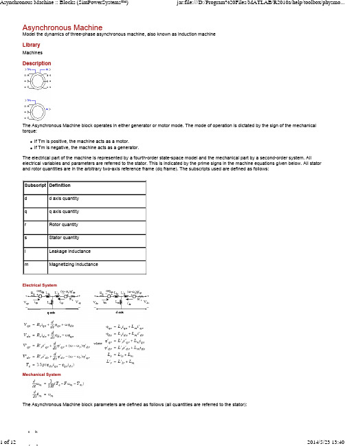
DescriptionThe Asynchronous Machine block operates in either generator or motor mode. The mode of operation is dictated by the sign of the mechanical torque:Mechanical Systems lsPreset modelProvides a set of predetermined electrical and mechanical parameters for various asynchronous machine ratings of power (HP),phase-to-phase voltage (V), frequency (Hz), and rated speed (rpm).Select one of the preset models to load the corresponding electrical and mechanical parameters in the entries of the dialog box. Note that the preset models do not include predetermined saturation parameters. Select No if you do not want to use a preset model, or if you want to modify some of the parameters of a preset model, as described below.When you select a preset model, the electrical and mechanical parameters in the Parameters tab of the dialog box become unmodifiable (grayed out). To start from a given preset model and then modify machine parameters, you have to do the following: Select the desired preset model to initialize the parameters.1.2.Change the Preset model parameter value to No. This will not change the machine parameters. By doing so, you just break theconnection with the particular preset model.3.Modify the machine parameters as you wish, then click Apply.Mechanical inputAllows you to select either the torque applied to the shaft or the rotor speed as the Simulink signal applied to the block's input.Select Torque Tm to specify a torque input, in N.m or in pu, and change labeling of the block's input to Tm. The machine speed isdetermined by the machine Inertia J (or inertia constant H for the pu machine) and by the difference between the applied mechanical torque Tm and the internal electromagnetic torque Te. The sign convention for the mechanical torque is the following: when the speed is positive,a positive torque signal indicates motor mode and a negative signal indicates generator mode.Select Speed w to specify a speed input, in rad/s or in pu, and change labeling of the block's input to w. The machine speed is imposed and the mechanical part of the model (Inertia J) is ignored. Using the speed as the mechanical input allows modeling a mechanicalcoupling between two machines and interfacing with SimMechanics™ and SimDriveline™ models.The next figure indicates how to model a stiff shaft interconnection in a motor-generator set when friction torque is ignored in machine 2.The speed output of machine 1 (motor) is connected to the speed input of machine 2 (generator), while machine 2 electromagnetic torque output Te is applied to the mechanical torque input Tm of machine 1. The Kw factor takes into account speed units of both machines (pu or rad/s) and gear box ratio w2/w1. The KT factor takes into account torque units of both machines (pu or N.m) and machine ratings. Also, asthe inertia J2 is ignored in machine 2, J2 referred to machine 1 speed must be added to machine 1 inertia J1.In the preceding equations, Θ is the angular position of the reference frame, while is the difference between the position of the reference frame and the position (electrical) of the rotor. Because the machine windings are connected in a three-wire Y configuration, The following table shows the values taken by Θ andframe).Specifies the units of the electrical and mechanical parameters of the model. This parameter is not modifiable; it is provided for informationpurposes only.Parameters TabNominal power, voltage (line-line), and frequencyThe nominal apparent power Pn (VA), RMS line-to-line voltage Vn (V), and frequency fn (Hz).Stator resistance and inductanceThe stator resistance Rs (Ω or pu) and leakage inductance Lls (H or pu).Rotor resistance and inductanceThe rotor resistance Rr' (Ω or pu) and leakage inductance Llr' (H or pu), both referred to the stator.Mutual inductanceThe magnetizing inductance Lm (H or pu).Inertia constant, friction factor, and pole pairs For the SI units dialog box: the combined machine and load inertia coefficient J (kg.m ), combined viscous friction coefficient F (N.m.s),and pole pairs p. The friction torque Tf is proportional to the rotor speed ω (Tf = F.w).For the pu units dialog box: the inertia constant H (s), combined viscous friction coefficient F (pu), and pole pairs p.Initial conditionsSpecifies the initial slip s, electrical angle Θe (degrees), stator current magnitude (A or pu), and phase angles (degrees):[slip, th, i , i , i , phase , phase , phase ]For the wound-rotor machine, you can also specify optional initial values for the rotor current magnitude (A or pu), and phase angles(degrees):[slip, th, i , i , i , phase , phase , phase , i , i , i ,phase , phase , phase ]For the squirrel cage machine, the initial conditions can be computed by the load flow utility in the Powergui block.Simulate saturationSpecifies whether magnetic saturation of rotor and stator iron is simulated or not.Saturation parametersSpecifies the no-load saturation curve parameters. Magnetic saturation of stator and rotor iron (saturation of the mutual flux) is modeled bya nonlinear function (in this case a polynomial) using points of the no-load saturation curve. You must enter a 2-by-n matrix, where n is thenumber of points taken from the saturation curve. The first row of this matrix contains the values of stator currents, while the second rowcontains values of corresponding terminal voltages (stator voltages). The first point (first column of the matrix) must correspond to the pointwhere the effect of saturation begins.2as bs cs as bs cs as bs cs as bs cs ar br cr ar br crSample time (-1 for inherited)Specifies the sample time used by the block. To inherit the sample time specified in the Powergui block, set this parameter to Inputs and OutputsTmThe Simulink input of the block is the mechanical torque at the machine's shaft. When the input is a positive Simulink signal, theconnected in series.When you use Asynchronous Machine blocks in discrete systems, you might have to use a small parasitic resistive load, connected at the machine terminals, in order to avoid numerical oscillations. Large sample times require larger loads. The minimum resistive load is proportional to the sample time. As a rule of thumb, remember that with a 25 μs time step on a 60 Hz system, the minimum load isThe 3 HP machine is connected to a constant load of nominal value (11.9 N.m). It is started and reaches the set point speed of 1.0 pu at t = 0.9 second.The parameters of the machine are those found in the SI Units dialog box above, except for the stator leakage inductance, which is set to twice its normal value. This is done to simulate a smoothing inductor placed between the inverter and the machine. Also, the stationary reference frame was used to obtain the results shown.Open the power_pwm demo. Note in the simulation parameters that a small relative tolerance is required because of the high switching rate of the inverter.Run the simulation and observe the machine's speed and torque.The first graph shows the machine's speed going from 0 to 1725 rpm (1.0 pu). The second graph shows the electromagnetic torque developed by the machine. Because the stator is fed by a PWM inverter, a noisy torque is observed.However, this noise is not visible in the speed because it is filtered out by the machine's inertia, but it can also be seen in the stator and rotor currents, which are observed next.the last moments of the simulation.Example 2: Effect of Saturation of the Asynchronous Machine BlockThe power_asm_sat demo illustrates the effect of saturation of the Asynchronous Machine block.Two identical three-phase motors (50 HP, 460 V, 1800 rpm) are simulated with and without saturation, to observe the saturation effects on thestator currents. Two different simulations are realized in the demo.The first simulation, is the no-load steady-state test. The table below contains the values of the Saturation Parameters obtained by simulating different operating points on the saturated motor (no-load and in steady-state).Saturation Parameters MeasurementsRunning the simulation with a blocked rotor or with many different values of load torque will allow the observation of other effects of saturation on the stator currents.References[1] Krause, P.C., O. Wasynczuk, and S.D. Sudhoff, Analysis of Electric Machinery, IEEE Press, 2002.[2] Mohan, N., T.M. Undeland, and W.P. Robbins, Power Electronics: Converters, Applications, and Design, John Wiley & Sons, Inc., New York, 1995, Section8.4.1.See AlsoPowerguiWas this topic helpful?Yes No© 1984-2010 The MathWorks, Inc. •Terms of Use•Patents•Trademarks•Acknowledgments。
课程设计--基于MATLABsimulink的三相交流异步电机正转和反转建模

课程设计--基于MATLABsimulink的三相交流异步电机正转和反转建模第一篇:课程设计--基于MATLABsimulink的三相交流异步电机正转和反转建模基于MATLAB/simulink的三相交流异步电机正转和反转建模与仿真姓名:李鹏程学号:031040525 专业:电气工程及其自动化完成日期:2012年12月18日[摘要] 在MATLAB/simulink环境下,设计和组合了三相交流异步电动机正转和反转的仿真模型。
仿真结果证明了控制方法的有效性,并且为其他交流异步电动机的设计提供了基本的设计理论的简单构型。
随着近年来电力电子工业和计算机科技的迅速发展,交流异步电动机赖于其结构简单,运行可靠,过载能力强,维护方便等优点逐渐应用于工业生产中的各个领域,并获得了广泛的接纳认可以及好评。
笔者仅仅基于简单的模块进行建模与仿真,从仿真模型中得出与实际理论相符合的情况,最终达到理论与实践相结合的目的。
一:三相交流电源模块设置以上为A项,相应的B、C两相相位分别改为120度、240度。
二:异步电动机参数设计设置转子以鼠笼式模块(squirrel-cage)进行连接,输出三相电流内部短路。
参考坐标系选用静止坐标系(stationary)。
异步电机的一切参数设置基于国家工频。
三:分路器设置其中包含:(1)定子三相电流:is-a、is-b。
is-c;(2)转子三相电流:ir-a、ir-b、ir-c;(3)转速n=wm/2pi;(4)转矩Te;这些量也是仿真中最后需要观察和分析的数据量。
四:完整的三相交流异步电机simulink模型异步电机simulink仿真模型1:仿真中必须有powergui模块。
其作用是:(1):可以显示系统稳定状态的电流和电压以及电路以及所有的状态变量值;(2):为了执行仿真,其可以允许修改初始状态值;(3):可以执行负载的潮流计算,可以初始化包括三相电机在内的三相网络,三相电机的简化模型为同步电机或异步电机。
基于MatlabSimulink的异步电机矢量控制系统仿真

基于MatlabSimulink的异步电机矢量控制系统仿真一、本文概述随着电力电子技术和控制理论的不断发展,异步电机矢量控制系统已成为现代电机控制领域的重要分支。
该系统通过精确控制异步电机的磁通和转矩,实现了对电机的高效、稳定和动态性能的优化。
Matlab/Simulink作为一种强大的仿真工具,为异步电机矢量控制系统的研究和设计提供了便捷的平台。
本文旨在探讨基于Matlab/Simulink的异步电机矢量控制系统仿真方法。
文章将简要介绍异步电机矢量控制的基本原理和关键技术,包括空间矢量脉宽调制(SVPWM)技术、转子磁链观测技术以及矢量控制策略等。
详细阐述如何利用Matlab/Simulink搭建异步电机矢量控制系统的仿真模型,包括电机模型、控制器模型以及系统仿真模型的构建过程。
文章还将探讨仿真模型的参数设置、仿真过程以及仿真结果的分析方法。
通过本文的研究,读者可以深入了解异步电机矢量控制系统的基本原理和仿真方法,掌握基于Matlab/Simulink的仿真技术,为异步电机矢量控制系统的实际设计和应用提供有益的参考和借鉴。
本文的研究也有助于推动异步电机矢量控制技术的发展和应用领域的拓展。
二、异步电机基本原理异步电机,又称感应电机,是一种广泛应用于工业领域的电动机。
其基本原理基于电磁感应和电磁力作用。
异步电机主要包括定子(静止部分)和转子(旋转部分)。
定子通常由铁芯和三相绕组构成,而转子则可能由实心铁芯、鼠笼型或绕线型结构组成。
当异步电机通电时,定子绕组中的三相电流会产生旋转磁场。
这个旋转磁场与转子中的导体相互作用,根据法拉第电磁感应定律,会在转子导体中产生感应电动势和感应电流。
这些感应电流在旋转磁场的作用下,受到电磁力的作用,从而使转子产生旋转力矩,驱动转子旋转。
异步电机的旋转速度与定子旋转磁场的旋转速度并不完全同步,这也是其被称为“异步”电机的原因。
异步电机的旋转速度通常略低于旋转磁场的同步速度,这是由于转子导体的电感和电阻导致的电磁延迟效应。
Simulink异步电机矢量控制(全文)
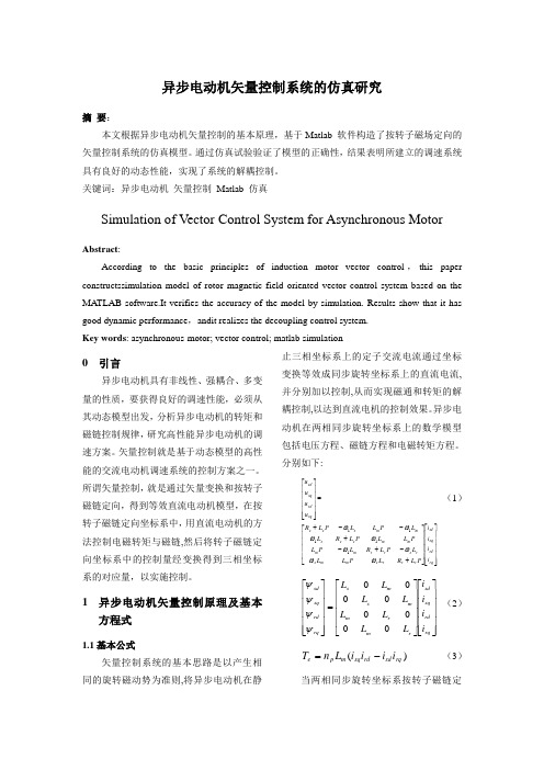
异步电动机矢量控制系统的仿真研究摘要:本文根据异步电动机矢量控制的基本原理,基于Matlab 软件构造了按转子磁场定向的矢量控制系统的仿真模型。
通过仿真试验验证了模型的正确性,结果表明所建立的调速系统具有良好的动态性能,实现了系统的解耦控制。
关键词:异步电动机矢量控制Matlab 仿真Simulation of Vector Control System for Asynchronous MotorAbstract:According to the basic principles of induction motor vector control,this paper constructssimulation model of rotor magnetic field oriented vector control system based on the MATLAB software.It verifies the accuracy of the model by simulation. Results show that it has good dynamic performance,andit realizes the decoupling control system.Key words: asynchronous-motor; vector control; matlab simulation0 引言异步电动机具有非线性、强耦合、多变量的性质,要获得良好的调速性能,必须从其动态模型出发,分析异步电动机的转矩和磁链控制规律,研究高性能异步电动机的调速方案。
矢量控制就是基于动态模型的高性能的交流电动机调速系统的控制方案之一。
所谓矢量控制,就是通过矢量变换和按转子磁链定向,得到等效直流电动机模型,在按转子磁链定向坐标系中,用直流电动机的方法控制电磁转矩与磁链,然后将转子磁链定向坐标系中的控制量经变换得到三相坐标系的对应量,以实施控制。
异步电机矢量控制Matlab仿真实验_(电机模型部分)

摘要异步电动机的动态数学模型是一个高阶、非线性、强耦合的多变量系统,由磁链方程、电压方程、转矩方程和运动方程组成,为非线性,所以控制起来极为不便。
异步电机的模型之所以复杂,关键在于各个磁通间的耦合。
如果把异步电动机模型解耦成有磁链和转速分别控制的简单模型,就可以模拟直流电动机的控制模型来控制交流电动机。
本文研究了按转子磁链定向的矢量控制系统的电流闭环控制的设计方法,通过坐标变换,在按转子磁链定向同步旋转正交坐标系中,得到等效的直流电动机模型,然后仿照直流电动机的控制方法控制电磁转矩与磁链,将转子磁链定向坐标系中的控制量反变换得到三相坐标系的对应量,以实施控制,并用MATLAB进行仿真。
关键词:异步电动机直流电动机磁链 MATLAB仿真目录1 课程任务设计书 (2)2 异步电动机数学模型基本原理 (3)2.1 异步电动机的三相动态数学模型 (3)2.2 异步电机的坐标变换 (6)2.2.1 三相-两相变换(3/2变换) (6)2.2.2静止两相-旋转正交变换(2s/2r变换) (8)3 异步电动机按转子磁链定向的矢量控制系统 (9)3.1 按转子磁链定向矢量控制的基本思想 (9)3.2 以ω-is-ψr 为状态变量的状态方程 (9)3.2.1 dq坐标系中的状态方程 (9)3.2.2αβ坐标系中的状态方程 (10)3.3αβ坐标系下异步电机的仿真模型 (11)3.4矢量控制系统设计 (14)3.5 矢量控制系统的电流闭环控制方式思想 (14)4 异步电动机矢量控制系统仿真 (15)4.1 仿真模型的参数计算 (15)4.2 矢量控制系统的仿真模型 (16)4.3仿真结果分析 (17)5. 总结与体会 (18)参考文献 (19)1课程任务设计书2 异步电动机数学模型基本原理异步电动机是个高阶、非线性、强耦合的多变量系统。
在研究异步电动机数学模型时,作如下的假设:120电角度,产生的磁动(1)忽略空间谐波,设三相绕组对称,在空间中互差势沿气隙周围按正弦规律分布;(2)忽略磁路饱和,各绕组的自感和互感都是恒定的;(3)忽略铁心饱和;(4)不考虑频率变化和温度变化对绕组电阻的影响。
基于MATLABSimulink的异步电机仿真

For personal use only in study and research; not for commercial use
基于MatlabSimulink的异步电机矢量控制系统仿真

基于Matlab/Simulink 的异步电机矢量控制系统仿真摘要在异步电机的数学模型分析中以及矢量控制系统的基础之上,利用Matlab/Simulink运用建立模块的思想分别组建了坐标变换模块、PI调节模块、转子磁链个观测模块、SVPWM等模块,然后将这些模块有机的结合,最后构成了异步电动机矢量控制的仿真模块,并且进行了仿真验证。
仿真结果分别显示了电机空载与负载情况下转矩、转速的动态变化曲线,验证了该方法的有效性、实用性,为电机在实际使用中打下了坚实的基础。
本文主要研究异步电机在矢量控制下的仿真。
使用Matlab/Simulink中的电气系统模块(PowerSystem Blocksets)将其重组得到新的模型并对其仿真,最后分析仿真结果得出结论。
关键词: 异步电机矢量控制 MATLAB/SIMULINK 变频调速目录摘要 (I)Abstract......................................................................................... 错误!未定义书签。
1 绪论 (1)1.1 电机及电力拖动技术的发展概况 (1)1.2 异步电动机的控制技术现状................................................. 错误!未定义书签。
1.3 仿真软件的简介及其选择..................................................... 错误!未定义书签。
1.4 论文的主要内容及结构安排................................................. 错误!未定义书签。
2 异步电动机的数学模型 (4)2.1 异步电动机的稳态数学模型 (4)2.2 异步电动机的动态数学模型 (5)2.3 本章小结 (7)3 矢量控制系统基本思路 (8)3.1 矢量控制的基本原理 (8)3.2 坐标变换 (9)3.3SVPWM调制 (21)3.3本章小结 (11)4 异步电机矢量控制系统仿真 (14)4.1矢量控制系统模型 (14)4.2仿真结果与分析 (15)4.5本章小结 (17)5结论与展望 (18)5.1结论 (18)5.2后续研究工作的展望 (19)参考文献 ....................................................................................... 错误!未定义书签。
基于matlab simulink的异步电动机交流调速系统模型设计及仿真
………………………. …………. …………………山东农业大学 毕 业 论 文 基于Matlab/Simulink 的异步电动机交流调速系统模型设计及仿真 院 部 机械与电子工程学院 专业班级 电气工程及其自动化3班 届 次 20**届 学生姓名 学 号 指导教师 二0**年六月一日装订线……………….……. …………. …………. ………目录摘要 (I)Abstract (II)1 绪论 (1)1.1 研究目的及意义 (1)1.1.1 研究目的 (1)1.1.2 研究意义 (1)1.2 研究的背景 (1)1.3 国内外研究现状 (1)1.4 研究方法 (2)2 异步电动机的调速系统 (2)2.1 异步电动机调速系统的分类 (2)2.2 异步电机调速原理简介 (3)2.2.1 变极电动机 (3)2.2.2 变频调速 (3)2.2.3 转子串电阻调速 (3)2.2.4 调压调速 (3)2.3 各种异步电机调速的特点 (3)2.3.1 变极调速方法 (3)2.3.2 变频调速方法 (3)2.3.3 转子串电阻调速方法 (4)2.3.4 调压调速的方法 (4)3 异步电机调压调速模型设计 (4)3.1 异步电机调压调速的原理 (4)3.2 速度负反馈的交流调压调速系统 (5)3.3 调压调速系统的组成部分 (6)3.3.1 三相交流调压器 (6)3.3.2 同步脉冲触发器 (7)3.3.3 反馈环节 (7)4 三相交流调压调速系统的matlab仿真 (9)4.1 matlab简介 (9)4.2 Simulink库介绍 (9)4.3系统建模与仿真 (11)4.3.1 三相电源的建模及参数设置 (11)4.3.2 同步流脉冲触发器的建模与参数的设置 (12)4.3.3 三相交流调压电路的建模与参数设置及仿真 (13)4.3.4 电机模块的建模与参数设置 (14)4.3.5 转速反馈环节及给定环节的建模及参数设置 (15)4.4 带转速负反馈的三相交流调压调速系统的连接图 (15)4.5 仿真结果与分析 (15)5 结论 (19)参考文献 (21)致谢 (22)附录 (23)ContentsAbstract ........................................................................................ 错误!未定义书签。
- 1、下载文档前请自行甄别文档内容的完整性,平台不提供额外的编辑、内容补充、找答案等附加服务。
- 2、"仅部分预览"的文档,不可在线预览部分如存在完整性等问题,可反馈申请退款(可完整预览的文档不适用该条件!)。
- 3、如文档侵犯您的权益,请联系客服反馈,我们会尽快为您处理(人工客服工作时间:9:00-18:30)。
DescriptionThe Asynchronous Machine block operates in either generator or motor mode. The mode of operation is dictated by the sign of the mechanical torque:Mechanical Systems lsPreset modelProvides a set of predetermined electrical and mechanical parameters for various asynchronous machine ratings of power (HP),phase-to-phase voltage (V), frequency (Hz), and rated speed (rpm).Select one of the preset models to load the corresponding electrical and mechanical parameters in the entries of the dialog box. Note that the preset models do not include predetermined saturation parameters. Select No if you do not want to use a preset model, or if you want to modify some of the parameters of a preset model, as described below.When you select a preset model, the electrical and mechanical parameters in the Parameters tab of the dialog box become unmodifiable (grayed out). To start from a given preset model and then modify machine parameters, you have to do the following: Select the desired preset model to initialize the parameters.1.2.Change the Preset model parameter value to No. This will not change the machine parameters. By doing so, you just break theconnection with the particular preset model.3.Modify the machine parameters as you wish, then click Apply.Mechanical inputAllows you to select either the torque applied to the shaft or the rotor speed as the Simulink signal applied to the block's input.Select Torque Tm to specify a torque input, in N.m or in pu, and change labeling of the block's input to Tm. The machine speed isdetermined by the machine Inertia J (or inertia constant H for the pu machine) and by the difference between the applied mechanical torque Tm and the internal electromagnetic torque Te. The sign convention for the mechanical torque is the following: when the speed is positive,a positive torque signal indicates motor mode and a negative signal indicates generator mode.Select Speed w to specify a speed input, in rad/s or in pu, and change labeling of the block's input to w. The machine speed is imposed and the mechanical part of the model (Inertia J) is ignored. Using the speed as the mechanical input allows modeling a mechanicalcoupling between two machines and interfacing with SimMechanics™ and SimDriveline™ models.The next figure indicates how to model a stiff shaft interconnection in a motor-generator set when friction torque is ignored in machine 2.The speed output of machine 1 (motor) is connected to the speed input of machine 2 (generator), while machine 2 electromagnetic torque output Te is applied to the mechanical torque input Tm of machine 1. The Kw factor takes into account speed units of both machines (pu or rad/s) and gear box ratio w2/w1. The KT factor takes into account torque units of both machines (pu or N.m) and machine ratings. Also, asthe inertia J2 is ignored in machine 2, J2 referred to machine 1 speed must be added to machine 1 inertia J1.In the preceding equations, Θ is the angular position of the reference frame, while is the difference between the position of the reference frame and the position (electrical) of the rotor. Because the machine windings are connected in a three-wire Y configuration, The following table shows the values taken by Θ andframe).Specifies the units of the electrical and mechanical parameters of the model. This parameter is not modifiable; it is provided for informationpurposes only.Parameters TabNominal power, voltage (line-line), and frequencyThe nominal apparent power Pn (VA), RMS line-to-line voltage Vn (V), and frequency fn (Hz).Stator resistance and inductanceThe stator resistance Rs (Ω or pu) and leakage inductance Lls (H or pu).Rotor resistance and inductanceThe rotor resistance Rr' (Ω or pu) and leakage inductance Llr' (H or pu), both referred to the stator.Mutual inductanceThe magnetizing inductance Lm (H or pu).Inertia constant, friction factor, and pole pairs For the SI units dialog box: the combined machine and load inertia coefficient J (kg.m ), combined viscous friction coefficient F (N.m.s),and pole pairs p. The friction torque Tf is proportional to the rotor speed ω (Tf = F.w).For the pu units dialog box: the inertia constant H (s), combined viscous friction coefficient F (pu), and pole pairs p.Initial conditionsSpecifies the initial slip s, electrical angle Θe (degrees), stator current magnitude (A or pu), and phase angles (degrees):[slip, th, i , i , i , phase , phase , phase ]For the wound-rotor machine, you can also specify optional initial values for the rotor current magnitude (A or pu), and phase angles(degrees):[slip, th, i , i , i , phase , phase , phase , i , i , i ,phase , phase , phase ]For the squirrel cage machine, the initial conditions can be computed by the load flow utility in the Powergui block.Simulate saturationSpecifies whether magnetic saturation of rotor and stator iron is simulated or not.Saturation parametersSpecifies the no-load saturation curve parameters. Magnetic saturation of stator and rotor iron (saturation of the mutual flux) is modeled bya nonlinear function (in this case a polynomial) using points of the no-load saturation curve. You must enter a 2-by-n matrix, where n is thenumber of points taken from the saturation curve. The first row of this matrix contains the values of stator currents, while the second rowcontains values of corresponding terminal voltages (stator voltages). The first point (first column of the matrix) must correspond to the pointwhere the effect of saturation begins.2as bs cs as bs cs as bs cs as bs cs ar br cr ar br crSample time (-1 for inherited)Specifies the sample time used by the block. To inherit the sample time specified in the Powergui block, set this parameter to Inputs and OutputsTmThe Simulink input of the block is the mechanical torque at the machine's shaft. When the input is a positive Simulink signal, theconnected in series.When you use Asynchronous Machine blocks in discrete systems, you might have to use a small parasitic resistive load, connected at the machine terminals, in order to avoid numerical oscillations. Large sample times require larger loads. The minimum resistive load is proportional to the sample time. As a rule of thumb, remember that with a 25 μs time step on a 60 Hz system, the minimum load isThe 3 HP machine is connected to a constant load of nominal value (11.9 N.m). It is started and reaches the set point speed of 1.0 pu at t = 0.9 second.The parameters of the machine are those found in the SI Units dialog box above, except for the stator leakage inductance, which is set to twice its normal value. This is done to simulate a smoothing inductor placed between the inverter and the machine. Also, the stationary reference frame was used to obtain the results shown.Open the power_pwm demo. Note in the simulation parameters that a small relative tolerance is required because of the high switching rate of the inverter.Run the simulation and observe the machine's speed and torque.The first graph shows the machine's speed going from 0 to 1725 rpm (1.0 pu). The second graph shows the electromagnetic torque developed by the machine. Because the stator is fed by a PWM inverter, a noisy torque is observed.However, this noise is not visible in the speed because it is filtered out by the machine's inertia, but it can also be seen in the stator and rotor currents, which are observed next.the last moments of the simulation.Example 2: Effect of Saturation of the Asynchronous Machine BlockThe power_asm_sat demo illustrates the effect of saturation of the Asynchronous Machine block.Two identical three-phase motors (50 HP, 460 V, 1800 rpm) are simulated with and without saturation, to observe the saturation effects on thestator currents. Two different simulations are realized in the demo.The first simulation, is the no-load steady-state test. The table below contains the values of the Saturation Parameters obtained by simulating different operating points on the saturated motor (no-load and in steady-state).Saturation Parameters MeasurementsRunning the simulation with a blocked rotor or with many different values of load torque will allow the observation of other effects of saturation on the stator currents.References[1] Krause, P.C., O. Wasynczuk, and S.D. Sudhoff, Analysis of Electric Machinery, IEEE Press, 2002.[2] Mohan, N., T.M. Undeland, and W.P. Robbins, Power Electronics: Converters, Applications, and Design, John Wiley & Sons, Inc., New York, 1995, Section8.4.1.See AlsoPowerguiWas this topic helpful?Yes No© 1984-2010 The MathWorks, Inc. •Terms of Use•Patents•Trademarks•Acknowledgments。