商务统计学(第四版)课后习题答案第八章
商务统计课后习题答案

Expected Price(Yi) 15 14 15 17 11 19 13 14 10 13 141
Totals
(Xi-X)2 Xi-X Yi-Y (Xi-X)(Yi-Y) -1.805 0.9 3.258025 -1.6245 2.195 -0.1 4.818025 -0.2195 0.011025 -0.105 0.9 -0.0945 3.783025 1.945 2.9 5.6405 -3.805 -3.1 14.47803 11.7955 6.795 4.9 46.172025 33.2955 -2.205 -1.1 4.862025 2.4255 -0.105 -0.1 0.011025 0.0105 -3.805 -4.1 14.478025 15.6005 0.895 -0.9 0.801025 -0.8055 92.67225 66.024
^
y = 0.275 + 0.95x
Texas Instruments has a higher risk. 53. a.
Satisfaction Rating(%) 100 80 60 Satisfaction Rating(%) 40 20 0 0 20 40 60 80
b. The relationship is positive. c. =43.92307692 y=65.92307692
b1=∑(Xi-X)(Yi-Y)/ ∑(Xi-X)2 =-170/1150 =-0.148 b0=y-b1 =17+.148*35=22.18
^
y=22.18-0.148x
b. SSR=25.1896 SSE=8.8696 MSR=SSR/Regression degrees of freedom=25.1896 MSE=SSE/n-2= 8.8696/4=2.2174 F=MSR/MSE=25.1896/2.2174=11.36 Fa=7.71<F
统计学课后习题答案_(第四版)4.5.7.8章
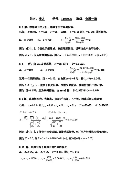
《统计学》第四版 第四章练习题答案4.1 (1)众数:M 0=10; 中位数:中位数位置=n+1/2=5.5,M e =10;平均数:6.91096===∑nxx i(2)Q L 位置=n/4=2.5, Q L =4+7/2=5.5;Q U 位置=3n/4=7.5,Q U =12 (3)2.494.1561)(2==-=∑-n i s x x (4)由于平均数小于中位数和众数,所以汽车销售量为左偏分布。
4.2 (1)从表中数据可以看出,年龄出现频数最多的是19和23,故有个众数,即M 0=19和M 0=23。
将原始数据排序后,计算中位数的位置为:中位数位置= n+1/2=13,第13个位置上的数值为23,所以中位数为M e =23(2)Q L 位置=n/4=6.25, Q L ==19;Q U 位置=3n/4=18.75,Q U =26.5(3)平均数==∑nx x i600/25=24,标准差65.612510621)(2=-=-=∑-n i s x x(4)偏态系数SK=1.08,峰态系数K=0.77(5)分析:从众数、中位数和平均数来看,网民年龄在23-24岁的人数占多数。
由于标准差较大,说明网民年龄之间有较大差异。
从偏态系数来看,年龄分布为右偏,由于偏态系数大于1,所以,偏斜程度很大。
由于峰态系数为正值,所以为尖峰分布。
4.3 (1(2)==∑nx x i63/9=7,714.0808.41)(2==-=∑-n i s x x (3)由于两种排队方式的平均数不同,所以用离散系数进行比较。
第一种排队方式:v 1=1.97/7.2=0.274;v 2=0.714/7=0.102.由于v 1>v 2,表明第一种排队方式的离散程度大于第二种排队方式。
(4)选方法二,因为第二种排队方式的平均等待时间较短,且离散程度小于第一种排队方式。
4.4 (1)==∑nx x i8223/30=274.1中位数位置=n+1/2=15.5,M e =272+273/2=272.5(2)Q L 位置=n/4=7.5, Q L ==(258+261)/2=259.5;Q U 位置=3n/4=22.5,Q U =(284+291)/2=287.5(3) 17.211307.130021)(2=-=-=∑-n i s x x4.5 (1)甲企业的平均成本=总成本/总产量=41.193406600301500203000152100150030002100==++++乙企业的平均成本=总成本/总产量=29.183426255301500201500153255150015003255==++++原因:尽管两个企业的单位成本相同,但单位成本较低的产品在乙企业的产量中所占比重较大,因此拉低了总平均成本。
商务统计习题解答.doc

4.49 4.33 (a)H = husband watching W= wife watching P(H\W) =商务统计习题解答4.41 (7)(3)(3)= 63〃! _ 7! _(7)(6)(5)X!(〃一 X )! 4!(3!)(3)(2)(1)P(WIH)・P(H) P(W I H)・P(H) + F(W 1H')・P(H')0.4 • 0.6 0.24 2 八 y0.4 • 0.6 + 0.3 • 0.4 - 036 ~ 3 - *(b) P(IV) = 0.24+0.12 =0.36 5.11 If p-0.25 and n = 5,(a) RX= 5) =0.0010(b) I\X> 4) = RX=4) + RX=5) = 0.0146+0.0010 =0.0156(c) 0) = 0.2373(d) F\X < 2) = RX=0) + RX= 1) + RX=2)=0.2373 + 0.3955 + 0.2637 = 0.89655.21(a) 0) = 0.0907 (b) RX= 1)=0.2177(c) I\X> 2)=0.6916 (d) RXv 3) = 0.56976.11 (a) P(X v 180) = P(Z v — 1.50) = 0.0668(b) P(180 v X v 300) = P(— 1.50 v Z v 1.50) = 0.9332 - 0.0668 = 0.8664(c) P( 110 v X v 180) = P(— 3.25 v Z v — 1.50) = 0.0668 - 0.00058 =0.06622(d) P(X v A) = 0.01 P(Z v - 2.33) = 0.01A = 240 - 2.33(40) = 146.80 seconds6.19(a) mean = 678.85, median = 675.5, range = 54,6(Sx ) =88.5734, interquartile range = 20, 1.33(S X ) = 19.6338 Since the mean is approximately equal to the median and the interquartile range isvery close to 1.33 times the standard deviation, the data appear to be approximatelynormally distributed.(b)710X±Z- 350±1.96- 100V64 325.5 < 辱 374.50The normal probability plot suggests that the data appear to be approximately normally distributed. 7.9 (a)P(叉 < 0.75) = P(Z < -1.3693) = 0.0855 (b)P(0.70 <X < 0.90) = P(—2.7386 <Z<2.7386) = 0.9938 (c) P(A< X < B) = P(- L2816 < Z < 1.2816) = 0.80A =0.8-1.2816 (0.0365) = 0.7532 B= 0.8 +1.2816 (0.0365) = 0.8468(d) P(X <A) = P(Z< 1.2816) = 0.90 A = 0.8 +1.2816 (0.0365) = 0.8468Note: The above answers are obtained using PHStat. They may be slightly different whenTable E.2 is used.7.19 (a) P(0.15 vp v0.25) = P(- 1.25 <Z< 1.25)=0.7887(b) P(A<p<B) = P(- 1.6449 <Z< 1.6449) = 0.90A = 0.2 - 1.6449(0.04) = 0.1342B = 0.2 + 1.6449(0.04) = 0.2658(c) P(A v p v B) = P(- 1.960<Z< 1.960) = 0.95A =0.2 - 1.960(0.04) = 0.12160.2+ 1.96(0.04) = 0.27848.8 (a)(b) No. The manufacturer cannot support a claim that the bulbs last an average 400 hours.Based on the data from the sample, a mean of 400 hours would represent a distanceof 4 standard deviations above the sample mean of 350 hours.(c) No. Since is known and n = 64, from the Central Limit Theorem, we may assumethat the sampling distribution of X is approximately normal.(d) The confidence interval is narrower based on a process standard deviation of 80hours rather than the original assumption of 100 hours.Normal Probability Plot690 680670660700650 -2 -1.5 -1 -0.5 0 0.51 Z Value 1.5 2a loo sMp(a)8.18 (a) X±F・S “,c 八4.6024 -7= = 23 ±2.0739•― 4nV23 $21.01 <//< $24.99一cr80~F= = 350 ± 1.96 • —f=X ± Z ・4tr V64(b) Based on the smaller standard deviation, a mean of 400 hours would represent adistance of 5 standard deviations above the sample mean of 350 hours. No,the manufacturer cannot support a claim that the bulbs have a mean life of400 hours.(b) You can be 95% confident that the mean bounced check fee for the population issomewhere between $21.01 and $24.99.又◊又 (\n 77 . 7〔P(l ? P n77 . j QA /0.77(0.23)8.28 (a) p= 0.77 p ± Z • ------------------------- =().77 ±1.96」 ------------------------------\ n V 10000.74 <7t< 0.80(b)p = 0.77 p ± Z •、格王=0.77 ± 1,645/wWV n v 10000.75 <7T< 0.79(c)The 95% confidence interval is wider. The loss in precision reflected as a widerconfidence interval is the price you have to pay to achieve a higher level ofconfidence.Z2<T2 1.962 - 40028.38 (a) n =——=-------------- -—— =245.86 Use n = 246& 50~, Z2cr2 1.962 -4002八”八TT八睥(b) n = ——-— = --------------- ---- =983.41 Use n = 984& 2529.30 (a) Ho: " =375 hours. The mean life of the manufacturers light bulbs isequal to 375 hours.H\: // #375 hours. The mean life of the manufacturer9s light bulbs differs from375 hours.Decision rule: Reject 仇if Z v - 1.96 or Z > + 1.96.Test statistic: Z =与人笔尹=-2.00Decision: Since Z c^ = 一2.00 is below the critical bound of - 1.96, reject There isenough evidence to conclude that the mean life of the manufacturer's light bulbsdiffers from 375 hours.(b) ^-value = 2(0.0228) = 0.0456.Interpretation: The probability of getting a sample of 64 light bulbs that will yielda mean life that is farther away from the hypothesized population mean than thissample is 0.0456-(c)Test statistic: t = s 商 315.33/应y!n<64 (d) The results are the same. The confidence interval formed does not include thehypothesized value of 375 hours.9.58 (a) H Q : // < 400 The mean life of the batteries is not more than 400 hours. H 、: 〃> 400 The mean life of the batteries is more than 400 hours.X 一以 473.46-400 t “ --------------- 7= = 7= = 1 .230 / s/y/n 210.77/J13 Decision: Since t < 1.7823, do not reject H 。
统计学贾俊平_第四版课后习题答案第八章
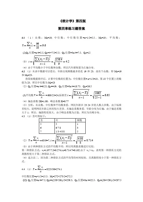
姓名:潘方 学号:1106026 班级:金融一班8.2 解:根据题目的分析,本题采用左单侧检验:已知:μ0=700,x =680,σ=60, n=36,α=0.05则z α=1.645 其过程为: H 0:μ≥700 H 1:μ<700 x z ==-2 因为|z|>|z α|,Z 值位于拒绝域,故拒绝原假设,说明这批产品不合格。
因为2=Z ,且为左单侧检验,则()05.0022750132.0977249868.01=<=-=αP8.4 解:由excel 计算得:x =99.9778 S =1.21221H 0:μ=100 H 1:μ≠100 x t =-0.055 这是一个双侧检验,当α=0.05,自由度n -1=9时,得()29t α=2.262。
因为t <|2t α|,t 值位于接受区域,故接受原假设,说明打包机工作正常。
因为|Z|=0.055,且为双侧检验,由excel 得: P=0.95734>(α=0.05)8.9解:该题样本为,大样本,方差2σ已知、且不等,因此采用z 统计量 已知, 05.0=α、即96.12/=αZ ,811=n , 642=n ,σA=63*63 2σB=57*57 0:211≠-μμH 0:210=-μμH , ()()96.15.0645781630102010702222<≈+--=+---=BB A AB A B A n n x x Z σσμμ 因为|z|<|z α|,Z 值位于接受区域,故接受原假设,两厂生产材料抗压强度相同。
因为5.0=Z ,则()=-⨯=691462461.012P 0.617075078()05.0=>α8.13 解:此题为两个总体比例之差的假设H 0:π1≥π2;H 1:π1<π 2 α=0.05,即z α=1.6451100021==n n ,00945.0110001041==p ,01718.0110001892==pp p d z --=0.009450.017180--=-5 因为|z|>|z α|,Z 值位于拒绝域,故拒绝原假设,说明用阿司匹林可以降低心脏病发生率。
统计学第四版课后答案
统计课后思考题答案第一章思考题什么是统计学统计学是关于数据的一门学科,它收集,处理,分析,解释来自各个领域的数据并从中得出结论。
解释描述统计和推断统计描述统计;它研究的是数据收集,处理,汇总,图表描述,概括与分析等统计方法。
推断统计;它是研究如何利用样本数据来推断总体特征的统计方法。
统计学的类型和不同类型的特点统计数据;按所采用的计量尺度不同分;(定性数据)分类数据:只能归于某一类别的非数字型数据,它是对事物进行分类的结果,数据表现为类别,用文字来表述;(定性数据)顺序数据:只能归于某一有序类别的非数字型数据。
它也是有类别的,但这些类别是有序的。
(定量数据)数值型数据:按数字尺度测量的观察值,其结果表现为具体的数值。
统计数据;按统计数据都收集方法分;观测数据:是通过调查或观测而收集到的数据,这类数据是在没有对事物人为控制的条件下得到的。
实验数据:在实验中控制实验对象而收集到的数据。
统计数据;按被描述的现象与实践的关系分;截面数据:在相同或相似的时间点收集到的数据,也叫静态数据。
时间序列数据:按时间顺序收集到的,用于描述现象随时间变化的情况,也叫动态数据。
解释分类数据,顺序数据和数值型数据答案同举例说明总体,样本,参数,统计量,变量这几个概念对一千灯泡进行寿命测试,那么这千个灯泡就是总体,从中抽取一百个进行检测,这一百个灯泡的集合就是样本,这一千个灯泡的寿命的平均值和标准差还有合格率等描述特征的数值就是参数,这一百个灯泡的寿命的平均值和标准差还有合格率等描述特征的数值就是统计量,变量就是说明现象某种特征的概念,比如说灯泡的寿命。
变量的分类变量可以分为分类变量,顺序变量,数值型变量。
变量也可以分为随机变量和非随机变量。
经验变量和理论变量。
举例说明离散型变量和连续性变量离散型变量,只能取有限个值,取值以整数位断开,比如“企业数”连续型变量,取之连续不断,不能一一列举,比如“温度”。
统计应用实例人口普查,商场的名意调查等。
商务统计学第八章

假设检验的实例与应用
实例1
某公司要检验新产品的广告效果 ,随机选取了100名顾客进行调 查。根据调查数据,公司可以得 出对广告效果的评价。
实例2
某制造商要检测其产品的质量, 随机选取了100个零件进行检测 。根据检测数据,制造商可以判 断产品质量是否符合标准。
实例3
某医院要评估某项治疗措施的效 果,随机选取了100名患者进行 治疗并对其疗效进行跟踪调查。 根据调查数据,医院可以得出对 该治疗措施的评价。
计算相关系数
使用相关系数公式计算两个变量之间的相关系数。
数据清洗
对收集到的数据进行预处理,包括缺失值处理、异常值处 理等。
判断相关程度
根据相关系数的取值范围,判断两个变量之间的相关程度 。
回归分析的基本概念
要点一
回归分析
是一种预测性的数据分析技术,通过研究变量之间的因 果关系,利用已知的自变量预测未知的因变量。
二项分布
n次独立重复试验中成功次数k 的概率分布,常用于描述有放回 抽样和伯努利试验的情形。
泊松分布
单位时间内发生随机事件的次数 的概率分布,常用于描述稀有事 件的发生概率。
04
大数定律与中心极限定理
大数定律的概念与性质
定义
大数定律是指当样本数量足够大时,随机 事件的频率呈现出一定的稳定性,即频率 的集中趋势明显。
计算数据集中每个观测值的算术 平均数,是描述数据集中趋势最 常用的指标。
中位数
将数据按大小排序后,位于中间 位置的数值即为中位数,适用于 偏态分布的数据。
众数
数据中出现次数最多的数值即为 众数,适用于具有明显偏态分布 的数据。
数据离散程度的度量
方差
反映数据离散程度的指标,数值越大表示数据越 离散。
商务统计学第八章习题
c) Both of the above.
d) None of the above.
ANபைடு நூலகம்WER:
c
TYPE: MC DIFFICULTY: Moderate
KEYWORDS: confidence interval, interpretation
4. If you were constructing a 99% confidence interval of the population mean based on a sample of
d) As the number of degrees of freedom increases, the t distribution approaches the normal
distribution.
ANSWER:
b) It is used to construct confidence intervals for the population mean when the population
standard deviation is known.
c) It is bell shaped and symmetrical.
a) narrower for 99% confidence than for 95% confidence.
b) wider for a sample size of 100 than for a sample size of 50.
c) narrower for 90% confidence than for 95% confidence.
----------------------------------
统计学课后习题答案(全章节)(精品).docx
第二章、练习题及解答2.为了确定灯泡的使用寿命(小时),在一批灯泡中随机抽取100只进行测试,所得结果如下:700 716 728 719 685 709 691 684 705 718 706 715 712 722 691 708 690 692 707 701 708 729 694 681 695 685 706 661 735 665 668 710 693 697 674 658 698 666 696 698 706 692 691 747 699 682 698 700 710 722 694 690 736 689 696 651 673 749 708 727 688 689 683 685 702 741 698 713 676 702 701 671 718 707 683 717 733 712 683 692 693 697 664 681 721 720 677 679 695 691 713 699 725 726 704 729 703 696 717 688要求:(2)以组距为10进行等距分组,生成频数分布表,并绘制直方图。
3.某公司下属40个销售点2012年的商品销售收入数据如下:单位:万元152 124 129 116 100 103 92 95 127 104 105 119 114 115 87 103 118 142 135 125 117 108 105 110 107 137 120 136 117 10897 88 123 115 119 138 112 146 113 126要求:(1)根据上面的数据进行适当分组,编制频数分布表,绘制直方图。
(2)制作茎叶图,并与直方图进行比较。
1.已知下表资料:25 20 10 500 2.5 30 50 25 1500 7.5 35 80 40 2800 14 40 36 18 1440 7.2 4514 7 630 3. 15 合 计200100687034. 35_y xf 6870根据频数计算工人平均日产量:〒=金^ =北* = 34.35 (件)£f 200结论:对同一资料,采用频数和频率资料计算的变量值的平均数是一致的。
统计学课后习题答案 第8章的习题答案
1. 解:根据题意建立原假设和备择假设:01:700;:700H H μμ≥<2x Z ===- 由于-2<-1.645,所以Z Z α<-,Z 值位于原假设0H 的拒绝域,所以拒绝0H ,即在显著性水平0.05下该批元件不合格。
2. 根据题意建立原假设和备择假设:01:250;:250H H μμ≤>20 3.336x t ====,0.05(24) 1.7109t =, 由于0.05(24),.t t t t α>>所以t 值位于原假设H 0,即在显著性水平0.05下该种化肥使得水稻明显增产。
3. 解:已知 0620.157,0.155,0.05, 1.96.400p p Z αα===== 根据题意建立原假设和备择假设:01:0.157;:0.157H P H P =≠0.10995P Z ===- -0.10995>-1.96,所以Z 值位于原假设H 0的接受域。
即在显著性水平0.05下随机调查的结果支持该市老年人口比重为15.7%。
4. 解:已知 09,100,99.98, 1.2122n x s μ====。
根据题意建立原假设和备择假设:01:100;:100H H μμ=≠0.020.04950.4041x t -====- -0.0495>-2.306,所以t 位于原假设H 0的接受域,即在显著性水平0.05下,打包机打包正常。
5. 解:已知00.05200,20,208.5,30,(19) 1.7291n x S t μ=====。
根据题意建立原假设和备择假设:01:200;:200H H μμ≤>8.5 1.2676.7083x t ==== t t α<,所以t 值位于原假设H 0的接受域,即在显著性水平0.05下,接受原假设,即在特定时间内每小时经过该地的汽车数量小于200辆。
6. 解:已知015,40,14.5, 2.3,0.05, 1.645n x S Z αμα======。
统计学(第四版)课后题答案
者比平均分数高 出 1 个标准差,而在 B 项测试中只高出平均分数 0.5 个标准差,由于 A 项 测试的标准化值高于 B 项测试,所以 A 项测试比较理想。 3.10 通过标准化值来判断,各天的标准化值如下表 日期 周一 周二 周三 周四 周五 周六 周日 标准化值 Z 3 -0.6 -0.2 0.4 -1.8 -2.2 0 周一和周六两天失去了控制。
-15~-10 10 -10~-5 13 -5~0 12 0~5 4 5~10 7 合计 60 (3)直方图(略) 。 2.9 (1)直方图(略) 。 (2)自学考试人员年龄的分布为右偏。 2.10(1)茎叶图如下
A班 数据个数 树 叶 树茎 B班 树叶 数据个数பைடு நூலகம்
0 3 59 2 1 4 4 0448 4 2 97 5 122456677789 12 11 97665332110 6 011234688 9 23 98877766555554443332100 7 00113449 8 7 6655200 8 123345 6 6 632220 9 011456 6 0 10 000 3 (2)A 班考试成绩的分布比较集中,且平均分数较高;B 班考试成绩的分 布比 A 班分散, 且平均成绩较 A 班低。 2.11(略) 。 2.12(略) 。 2.13(略) 。 2.14(略) 。 2.15箱线图如下: (特征请读者自己分析)
2 4.1 (1)200。 (2)5。 (3)正态分布。 (4) (100 1) 。
4.2 (1)32。 (2)0.91。 4.3 0.79。 4.4 (1) x 25 ~ N (17,2 2 ) 。 (2) x100 ~ N (17,1) 。 4.5 (1)1.41。 (2)1.41,1.41,1.34。 4.6 (1)0.4。 (2)0.024 。 (3)正态分布。 4.7 (1)0.050,0.035,0.022,016。 (2)当样本量增大时,样本比例的标准 差越来越小。 4.8 (1) (2)E=4.2; (3) (115.8,124.2) 。 x 2.14 ; 4.9 (87819,121301) 。 4.10(1)81±1.97; (2)81±2.35; (3)81±3.10。 4.11(1) (24.11,25.89) ; (2) (113.17,126.03) ; (3) (3.136,3.702) 4.12(1) (8687,9113) ; (2) (8734 ,9066) ; (3) (8761,9039) ; (4) (8682, 9118) 。 4.13(2.88,3.76) ;(2.80,3.84);(2.63,4.01)。 4.14(7.1,12.9) 。 4.15(7.18,11.57) 。 4.16(1) (148.9,150.1) ; (2)中心极限定理。 4.17(1) (100.9,123.7) ; (2) (0.017,0.183) 。 4.18(15.63,16.55) 。 4.19(10.36,16.76) 。
- 1、下载文档前请自行甄别文档内容的完整性,平台不提供额外的编辑、内容补充、找答案等附加服务。
- 2、"仅部分预览"的文档,不可在线预览部分如存在完整性等问题,可反馈申请退款(可完整预览的文档不适用该条件!)。
- 3、如文档侵犯您的权益,请联系客服反馈,我们会尽快为您处理(人工客服工作时间:9:00-18:30)。
CHAPTER 88.1 X ±Z ⋅σn= 85±1.96⋅864 83.04 ≤µ≤ 86.968.2 X ±Z ⋅σn= 125±2.58⋅2436114.68 ≤µ≤ 135.328.3 If all possible samples of the same size n are taken, 95% of them include the true population average monthly sales of the product within the interval developed. Thus you are 95 percent confident that this sample is one that does correctly estimate the true average amount. 8.4Since the results of only one sample are used to indicate whether something has gone wrong in the production process, the manufacturer can never know with 100% certainty that the specific interval obtained from the sample includes the true population mean. In order to have 100% confidence, the entire population (sample size N ) would have to be selected.8.5To the extent that the sampling distribution of sample means is approximately normal, it is true that approximately 95% of all possible sample means taken from samples of that same size will fall within 1.96 times the standard error away from the true population mean. But the population mean is not known with certainty. Since the manufacturer estimated the mean would fall between 10.99408 and 11.00192 inches based on a single sample, it is not necessarily true that 95% of all sample means will fall within those same bounds. 8.6 Approximately 5% of the intervals will not include the true population. Since the true population mean is not known, we do not know for certain whether it is contained in the interval (between 10.99408 and 11.00192 inches) that we have developed.8.7 (a) X ±Z ⋅σn=0.995±2.58⋅0.02500.9877≤µ≤1.0023(b) Since the value of 1.0 is included in the interval, there is no reason to believe that the mean is different from 1.0 gallon.(c) No. Since σ is known and n = 50, from the Central Limit Theorem, we may assume that the sampling distribution of X is approximately normal.(d) The reduced confidence level narrows the width of the confidence interval.X ±Z ⋅σn=0.995±1.96⋅0.02500.9895≤µ≤1.0005(b)Since the value of 1.0 is still included in the interval, there is no reason to believe that the mean is different from 1.0 gallon.8.8 (a)350 1.96X Z ±=± 325.5≤µ≤374.50(b) No. The manufacturer cannot support a claim that the bulbs last an average 400 hours. Based on the data from the sample, a mean of 400 hours would represent a distance of 4 standard deviations above the sample mean of 350 hours.(c)No. Since σ is known and n = 64, from the Central Limit Theorem, we may assume that the sampling distribution of X is approximately normal.(d) The confidence interval is narrower based on a process standard deviation of 80hours rather than the original assumption of 100 hours.(a)X ±Z ⋅σn=350±1.96⋅8064330.4≤µ≤369.6(b)Based on the smaller standard deviation, a mean of 400 hours wouldrepresent a distance of 5 standard deviations above the sample mean of 350 hours. No, the manufacturer cannot support a claim that the bulbs have a mean life of 400 hours.8.9 (a) X ±Z ⋅σn=1.99±1.96⋅0.051001.9802≤µ≤1.9998 (b) No. Since σ is known and n = 100, from the central limit theorem, we may assume thatthe sampling distribution of X is approximately normal.(c) An individual value of 2.02 is only 0.60 standard deviation above the sample mean of 1.99. The confidence interval represents bounds on the estimate of the average of a sample of 100, not an individual value.(d)A shift of 0.02 units in the sample average shifts the confidence interval by the same distance without affecting the width of the resulting interval.(a)X ±Z ⋅σn=1.97±1.96⋅0.051001.9602≤µ≤1.97988.10 (a) t 9 = 2.2622 (b) t 9 = 3.2498 (c) t 31 = 2.0395 (d) t 64 = 1.9977 (e) t 15 = 1.75318.11 75 2.0301X t ±=± 66.8796 ≤µ≤ 83.1204 8.12 50 2.9467X t ±=± 38.9499 ≤µ≤ 61.05018.13 Set 1: 4.5±2.3646⋅3.74178 1.3719 ≤µ≤ 7.6281 Set 2: 4.5±2.3646⋅2.449582.4522 ≤µ≤ 6.5478The data sets have different confidence interval widths because they have different values forthe standard deviation.8.14 Original data:5.8571±2.4469⋅6.46607 – 0.1229 ≤µ≤ 11.8371 Altered data: 4.00±2.4469⋅2.160272.0022 ≤µ≤ 5.9978The presence of an outlier in the original data increases the value of the sample mean and greatly inflates the sample standard deviation.8.15 (a) 1.67 2.0930X t ±=± $1.52 ≤µ≤ $1.82(b)The store owner can be 95% confident that the population mean retail value ofgreeting cards that the store has in its inventory is somewhere in between $1.52 and $1.82. The store owner could multiply the ends of the confidence interval by the number of cards to estimate the total value of her inventory.8.16 (a) 32 2.0096X t ±=± 29.44 ≤µ≤ 34.56 (b) The quality improvement team can be 95% confident that the population meanturnaround time is somewhere in between 29.44 hours and 34.56 hours.(c)The project was a success because the initial turnaround time of 68 hours does not fall inside the 95% confidence interval.8.17 (a) 195.3 2.1098X t ±=±≤µ≤ 205.9419 (b)No, a grade of 200 is in the interval.(c) It is not unusual. A tread-wear index of 210 for a particular tire is only 0.69 standard deviation above the sample mean of 195.3.8.18 (a) 23 2.0739X t ±=±≤µ≤ $24.99 (b) You can be 95% confident that the mean bounced check fee for the population issomewhere between $21.01 and $24.99.8.19 (a)7.1538 2.0595X t ±=±≤µ≤ $8.39 (b)You can be 95% confident that the population mean monthly service fee, if acustomer’s account falls below the minimum required balance, is somewhere between $5.92 and $8.39.8.20 (a)43.04 2.0096X t ±=±≤µ≤ 54.96 (b) The population distribution needs to be normally distribution.(c)Normal Probability Plot-3-2-10123Z ValueDa y sBox-and-whisker Plot050100150Both the normal probability plot and the box-and-whisker plot suggest that the distribution is skewed to the right.(d)Even though the population distribution is not normally distributed, with a sample of 50, the t distribution can still be used due to the Central Limit Theorem.8.21 (a)43.8889 2.0555X t ±=± 33.89 ≤µ≤ 53.89 (b) The population distribution needs to be normally distributed.(c)Box-and-whisker Plot1030507090Normal Probability Plot0102030405060708090100-2-1.5-1-0.50.511.52Z ValueT i m eBoth the normal probability plot and the box-and-whisker show that the population distribution is not normally distributed and is skewed to the right.8.22 (a)182.4 2.0930X t ±=± $161.68 ≤µ≤ $203.12(b) 45 2.0930X t ±=± $40.31 ≤µ≤ $49.69(c)The population distribution needs to be normally distributed.8.22 (d) cont.Normal Probability Plot050100150200250300-2-1.5-1-0.50.511.52Z ValueH o t e lBox-and-whisker Plot110160210260310Both the normal probability plot and the box-and-whisker show that the population distribution for hotel cost is not normally distributed and is skewed to the right.8.22 (d) cont.Normal Probability Plot010********607080-2-1.5-1-0.500.511.52Z ValueC a r sBox-and-whisker Plot3040506070Both the normal probability plot and the box-and-whisker show that the population distribution for rental car cost is not normally distributed and is skewed to the right.8.23 (a)0.00023 1.9842X t ±=−± –0.000566 ≤µ≤ 0.000106(b)The population distribution needs to be normally distributed. However, with a sampleof 100, the t distribution can still be used as a result of the Central Limit Theorem even if the population distribution is not normal.(c)Both the normal probability plot and the box-and-whisker plot suggest that the distribution is skewed to the right.(d)We are 95% confident that the mean difference between the actual length of the steel part and the specified length of the steel part is between -0.000566 and 0.000106 inches, which is narrower than the plus or minus 0.005 inches requirement. The steel mill is doing a good job at meeting the requirement. This is consistent with the finding in Problem 2.23.Normal Probability Plot-0.004-0.003-0.002-0.00100.0010.0020.0030.0040.0050.006Z ValueE r r orBox-and-whisker Plot-0.006-0.004-0.00200.0020.0040.0068.2450200X p n === 0.25 0.25p Z ±=±0.19 π≤≤ 0.318.2525400X p n === 0.0625 0.0625p Z ±=± 0.0313 0.09378.26 (a)135500X p n === 0.27 0.27p Z ±=±0.22π≤≤ 0.32(b)The manager in charge of promotional programs concerning residential customers can infer that the proportion of households that would purchase an additionaltelephone line if it were made available at a substantially reduced installation cost is between 0.22 and 0.32 with a 99% level of confidence.8.27 (a) 330500X p n === 0.66 0.66p Z ±=± 0.62 π≤≤ 0.70(b) You can be 95% confident that the population proportion of highly educated womenwho left careers for family reasons that want to return to work is between 0.62 and 0.70.8.28 (a) p = 0.77 0.77p Z ±=±0.74 π≤≤ 0.80(b) p = 0.77 0.77p Z ±=± 0.75 π≤≤ 0.79(c) The 95% confidence interval is wider. The loss in precision reflected as a widerconfidence interval is the price you have to pay to achieve a higher level of confidence.8.29 (a) p = 0.27 0.27p Z ±=±0.25 π≤≤ 0.29 (b)You can be 95% confident that the population proportion of older consumers that don’t think they have enough time to be good money managers is somewhere between 0.25 and 0.29.8.30 (a)0.46Xp n== 0.46p Z ±=±0.41630.5037π<<(b) 0.10Xp n== 0.10p Z ±=±0.07370.1263π<<8.31 (a) p = 0.2697 0.2697p Z ±=±0.24 π≤≤ 0.30(b) p = 0.2697 0.2697p Z ±=±0.23π≤≤ 0.31 (c)The 99% confidence interval is wider. The loss in precision reflected as a widerconfidence interval is the price one has to pay to achieve a higher level of confidence.8.32 (a) 4500.451000X p n ===0.45p Z ±=±0.41920.4808π<<(b) You are 95% confidence that the proportion of all working women in North America who believe that companies should hold positions for those on maternity leave for more than six months is between 0.4192 and 0.4808.298 Chapter 8: Confidence Interval Estimation8.33 (a)1260.21600X p n === 0.21p Z ±=±0.18π≤≤ 0.24(b)1260.21600X p n === 0.21p Z ±=±0.17π≤≤ 0.25 (c) You are 95% confidence that the population proportion of employers who have amandatory mail order program in place or are adopting one by the end of 2004 is between 0.18 and 0.24.You are 99% confidence that the population proportion of employers who have amandatory mail order program in place or are adopting one by the end of 2004 is between 0.17 and 0.25.(d)When the level of confidence is increased, the confidence interval becomes wider. The loss in precision reflected as a wider confidence interval is the price youhave to pay to achieve a higher level of confidence.8.34 n =Z 2σ2e 2=1.962⋅15252= 34.57 Use n = 358.35 n =Z 2σ2e 2=2.582⋅1002202= 166.41 Use n = 1678.36 2222(1–) 2.58(0.5)(0.5)(0.04)Z n e ππ== = 1,040.06Use n = 1,0418.37 2222(1–) 1.96(0.4)(0.6)(0.02)Z n e ππ== = 2,304.96Use n = 2,3058.38 (a) n =Z 2σ2e 2=1.962⋅4002502= 245.86 Use n = 246 (b) 2222221.9640025Z n eσ⋅== = 983.41 Use n = 9848.39 n =Z 2σ2e 2=1.962⋅(0.02)2(0.004)2= 96.04 Use n = 978.40 n =Z 2σ2e 2=1.962⋅(100)2(20)2= 96.04 Use n = 978.41 n =Z 2σ2e 2=1.962⋅(0.05)2(0.01)2= 96.04 Use n = 97Solutions to End-of-Section and Chapter Review Problems 2998.42 (a) n =Z 2σ2e 2=2.582⋅25252= 166.41 Use n = 167 (b) n =Z 2σ2e 2=1.962⋅25252= 96.04 Use n = 978.43 (a) n =Z 2σ2e 2=1.6452⋅45252= 219.19 Use n = 220 (b) n =Z 2σ2e 2=2.582⋅45252= 539.17 Use n = 5408.44 n =Z 2σ2e 2=1.962⋅20252= 61.47 Use n = 628.45 (a) 2222(1–) 1.96(0.1577)(10.1577)(0.06)Z n e ππ−== = 141.74 Use n = 142 (b) 2222(1–) 1.96(0.1577)(10.1577)(0.04)Z n e ππ−== = 318.91 Use n = 319 (c) 2222(1–) 1.96(0.1577)(10.1577)(0.02)Z n eππ−== = 1275.66 Use n = 12768.46 (a) 2222(1) 1.96(0.45)(0.55)(0.02)Z n e ππ−== = 2376.8956 Use n = 2377 (b) 2222(1) 1.96(0.29)(0.71)(0.02)Z n eππ−== = 1977.3851 Use n = 1978(c) The sample sizes differ because the estimated population proportions are different.(d)Since purchasing groceries at wholesale clubs and purchasing groceries at convenience stores are not necessary mutually exclusive events, it is appropriate to use one sample and ask the respondents both questions. However, drawing two separate samples is also appropriate for the setup.8.47 (a) 2222(1) 1.96(0.35)(10.35)546.2068(0.04)Z n eππ−−=== Use n = 547 (b) ()22222.5758(0.35)(10.35)(1)943.4009(0.04)Z n e ππ−−=== Use n = 944(c)2222(1) 1.96(0.35)(10.35)2184.8270(0.02)Z n e ππ−−=== Use n = 2185 (d) ()22222.5758(0.35)(10.35)(1)3773.6034(0.02)Z n e ππ−−=== Use n = 3774(e)Holding everything else constant, the higher the confidence level desired or the lowerthe acceptable sampling error, the larger the sample size needed.300 Chapter 8: Confidence Interval Estimation8.48 (a) 3030.9294326X p n ===0.9294 1.96p Z ±=±0.90170.9572π≤≤(b)You are 95% confident that the population proportion of business men and women whohave their presentations disturbed by cell phones is between 0.9017 and 0.9572.(c) 2222(1) 1.96(0.9294)(10.9294)157.5372(0.04)Z n e ππ−−=== Use n = 158(d)2222(1) 2.5758(0.9294)(10.9294)272.0960(0.04)Z n e ππ−−=== Use n = 2738.49 (a) 0.52 1.96p Z ±=±0.50530.5347π≤≤(b)You are 95% confident that the proportion of families that held stocks in 2001 isbetween 0.5053 and 0.5347.(c) 2222(1) 1.96(0.52)(10.52)9588.2695(0.01)Z n e ππ−−=== Use n = 95898.50The only way to have 100% confidence is to obtain the parameter of interest, rather than a sample statistic. From another perspective, the range of the normal and t distribution is infinite, so a Z or t value that contains 100% of the area cannot be obtained.8.51 The t distribution is used for obtaining a confidence interval for the mean when σ isunknown. 8.52 If the confidence level is increased, a greater area under the normal or t distribution needs to be included. This leads to an increased value of Z or t , and thus a wider interval.8.53When estimating the rate of noncompliance, it is commonplace to use a one-sided confidence interval instead of a two-sided confidence interval since only the upper bound on the rate of noncompliance is of interest.8.54 In some applications such as auditing, interest is primarily on the total amount of a variable rather than the mean amount.8.55 Difference estimation involves determining the difference between two amounts, rather than a single amount.Solutions to End-of-Section and Chapter Review Problems 3018.56 (a) The population from which this sample was drawn was the collection of all the people who visited the magazine's web site.(b) The sample is not a random sample from this population. The sample consisted of only those who visited the magazine's web site and chose to fill out the survey. (c)This is not a statistically valid study. There was selection bias since only those who visited the magazine's web site and chose to answer the survey were represented. There was possibly nonresponse bias as well. Visitors to the web site who chose to fill out the survey might not answer all questions and there was no way for the magazine to get back to them to follow-up on the nonresponses if this was an anonymous survey.(d)To avoid the above potential pitfalls, the magazine could have drawn a random sample from t he list of all subscribers to the magazine and offer them the option of filling out the survey over the Internet or on the survey form that is mailed to the subscribers. The magazine should also keep track of the subscribers who are invited to fill out the survey and follow up on the nonresponses after a specified period of time with mail or telephone to encourage them to participate in the survey.The sample size needed is 2222(1) 1.96(0.6195)(10.6195)2264(0.02)Z n e ππ⋅⋅−⋅⋅−===8.57 (a) 0.44 1.96p Z ±=± 0.39650.4835π<<(b)Since the range that covers 0.5 and above is not contained in the 95% confidenceinterval, we can conclude that less than half of all applications contain inaccuracies with past employers.(c)0.44 1.96p Z ±=± 0.37120.5088π<<(d) Since the 95% confidence interval contains 0.5, it is incorrect to conclude that lessthan half of all applications contain inaccuracies with past employers.(e)The smaller sample size in (c) results in a wider confidence interval and, hence, results in a loss of precision in the interval estimate.8.58 (a) 0.58 1.96p Z ±=±0.51160.6484π<<(b) 0.50 1.96p Z ±=±0.43070.5693π<<(c) 0.22 1.96p Z ±=±0.16260.2774π<<(d)0.19 1.96p Z ±=±0.13560.2444π<<(e) 2222(1) 1.96(0.5)(0.5)2400.92401(0.02)Z n eππ⋅⋅−⋅⋅===≅302 Chapter 8: Confidence Interval Estimation8.59 Cheat at golf:0.8204 1.96p Z ±=± 0.78290.8580π<<Hate others who cheat at golf:0.8204 1.96p Z ±=± 0.78290.8580π<<Believe business and golf behavior parallel:0.7207 1.96p Z ±=± 0.67680.7646π<<Would let a client win to get business:0.1995 1.96p Z ±=± 0.16040.2386π<<Would call in sick to play golf:0.0998 1.96p Z ±=±0.07040.1291π<<From these confidence intervals, we can conclude with 95% level of confidence that more thanhalf of the CEOs will cheat at golf, hate others who cheat at golf and believe business and golf behavior parallel and less than half of the CEOs will let a client win to get business or call in sick to play golf.8.60 (a) 15.3 2.0227X t ±=± 14.085 ≤µ≤ 16.515(b)0.675 1.96p Z ±=± 0.530 π≤≤ 0.820 (c) n =Z 2⋅σ2e 2=1.962⋅5222= 24.01 Use n = 25(d) 2222(1–) 1.96(0.5)(0.5)(0.035)Z n eππ⋅⋅⋅⋅== = 784 Use n = 784(e)If a single sample were to be selected for both purposes, the larger of the two samplesizes (n = 784) should be used.8.61 (a) 1759 2.6490X t ±=± 1,638.69 ≤µ≤ 1,879.31(b)0.60 1.96p Z ±=±π≤≤ 0.715Solutions to End-of-Section and Chapter Review Problems 3038.62 (a) 9.7 2.0639X t ±=± 8.049 ≤µ≤ 11.351(b)0.48 1.96p Z ±=±π≤≤ 0.676 (c) n =Z ⋅e 2=1.962⋅4.521.52= 34.57 Use n = 35 (d) 2222(1–) 1.645(0.5)(0.5)(0.075)Z n e ππ⋅⋅⋅⋅== = 120.268 Use n = 121 (e)If a single sample were to be selected for both purposes, the larger of the two samplesizes (n = 121) should be used.8.63 (a) n =Z 2⋅σ2e 2=2.582⋅18252= 86.27Use n = 87Note : If the Z -value used is carried out to 2.5758, the value of n is 85.986 and only 86 women would need to be sampled.(b)2222(1–) 1.645(0.5)(0.5)(0.045)Z n e ππ⋅⋅⋅⋅== = 334.07 Use n = 335(c)If a single sample were to be selected for both purposes, the larger of the two samplesizes (n = 335) should be used.8.64 (a) $28.52 1.9949X t ±=± $25.80 ≤µ≤ $31.24(b)0.40 1.645p Z ±=±π≤≤ 0.4963 (c) n =Z ⋅σe 2=1.962⋅10222= 96.04 Use n = 97 (d) 2222(1–) 1.645(0.5)(0.5)(0.04)Z n e ππ⋅⋅⋅⋅== = 422.82 Use n = 423 (e) If a single sample were to be selected for both purposes, the larger of the two samplesizes (n = 423) should be used.8.65 (a) $21.34 1.9949X t ±=± $19.14 ≤µ≤ $23.54(b) 0.3714 1.645p Z ±=±0.2764 π≤≤ 0.4664(c)n =Z 2⋅σ2e 2=1.962⋅1021.52= 170.74 Use n = 171 (d)2222(1–) 1.645(0.5)(0.5)(0.045)Z n e ππ⋅⋅⋅⋅== = 334.08 Use n = 335304 Chapter 8: Confidence Interval Estimation8.65 (e) If a single sample were to be selected for both purposes, the larger of the two sample cont. sizes (n = 335) should be used.8.66 (a)$38.54 2.0010X t ±=±≤µ≤ $40.42(b) 0.30 1.645p Z ±=±π≤≤ 0.3973 (c) n =Z 2⋅σ2e 2=1.962⋅821.52= 109.27 Use n = 110 (d) 2222(1–) 1.645(0.5)(0.5)(0.04)Z n e ππ⋅⋅⋅⋅== = 422.82 Use n = 423 (e)If a single sample were to be selected for both purposes, the larger of the two samplesizes (n = 423) should be used.8.67 (a) 2222(1) 1.96(0.5)(0.5)(0.05)Z n eππ⋅⋅−⋅⋅== = 384.16 Use n = 385If we assume that the population proportion is only 0.50, then a sample of 385 wouldbe required. If the population proportion is 0.90, the sample size required is cut to 103.(b) 0.84 1.96p Z ±=± 0.7384≤ π ≤ 0.9416 (c) The representative can be 95% confidence that the actual proportion of bags that will dothe job is between 74.5% and 93.5%. He/she can accordingly perform a cost-benefit analysis to decide if he/she wants to sell the Ice Melt product.8.68 (a) 8.4209 2.0106X t ±=± 8.418.43µ≤≤(b) With 95% confidence, the population mean width of troughs is somewhere between 8.41and 8.43 inches. Hence, the company's requirement of troughs being between 8.31 and 8.61 is being met with a 95% level of confidence.8.69 (a) 5.5014 2.6800X t ±=± 5.46 5.54µ≤≤(b) Since 5.5 grams is within the 99% confidence interval, the company can claim that themean weight of tea in a bag is 5.5 grams with a 99% level of confidence.Solutions to End-of-Section and Chapter Review Problems 3058.70 (a)0.2641 1.9741X t ±=±0.24250.2856µ≤≤(b)0.218 1.9772X t ±=±0.19750.2385µ≤≤(c)Normal Probability Plot00.10.20.30.40.50.60.70.80.9-3-2-1123Z ValueV e r m o n tNormal Probability Plot00.20.40.60.811.2-3-2-1123Z ValueB o s t o nThe amount of granule loss for both brands are skewed to the right.(d)Since the two confidence intervals do not overlap, we can conclude that the mean granule loss of Boston shingles is higher than that of Vermont Shingles.306 Chapter 8: Confidence Interval Estimation8.71 (a)3124.2147 1.9665X t ±=±3120.663127.77µ≤≤(b)3704.0424 1.9672X t ±=± 3698.98<3709.10µ<(c)Normal Probability Plot3000305031003150320032503300-4-3-2-11234Z ValueB o s t o nNormal Probability Plot35503600365037003750380038503900-4-3-2-11234Z ValueV e r m o n tThe weight for Boston shingles is slightly skewed to the right while the weight for Vermont shingles appears to be slightly skewed to the left.(d)Since the two confidence intervals do not overlap, the mean weight of Vermont shingles is greater than the mean weight of Boston shingles.Solutions to End-of-Section and Chapter Review Problems 3078.72(a)NY, Food: 20.1 2.0096X t ±=± 19.5120.69µ≤≤ LI, 20.54 2.0096X t ±=± 19.7321.35µ≤≤ NY, 17.12 2.0096X t ±=± 16.3517.89µ≤≤ LI, 17.64 2.0096X t ±=± 16.6518.63µ≤≤ NY, 18.4 2.0096X t ±=± 17.7419.06µ≤≤ LI, 19.04 2.0096X t ±=±18.3719.71µ≤≤NY, 39.74 2.0096X t ±=± 37.0042.48µ≤≤ LI, 33.7400 2.0096X t ±=± 31.5535.93µ≤≤(b)With 95% confidence you can conclude the mean price per person in New York City isgreater than the mean in Long Island. With 95% confidence you can conclude that there are no differences in the ratings for food, décor and service between the two cities.。