双向流固耦合实例
流固耦合计算实例
Oscillating Plate with Two-Way Fluid-Structure InteractionANSYS-ChinaIntroductionThis tutorial includes:∙Features∙Overview of the Problem to Solve∙Setting up the Solid Physics in Simulation (ANSYS Workbench)∙Setting up the Fluid Physics and ANSYS Multi-field Settings in ANSYS CFX-Pre∙Obtaining a Solution using ANSYS CFX-Solver Manager∙Viewing Results in ANSYS CFX-PostIf this is the first tutorial you are working with, it is important to review the following topics before beginning:∙Setting the Working Directory∙Changing the Display ColorsUnless you plan on running a session file, you should copy the sample files used in this tutorial from the installation folder for your software (<CFXROOT>/examples/) to your working directory. This prevents you from overwriting source files provided with your installation. If you plan to use a session file, please refer to Playing a Session File.Sample files referenced by this tutorial include:∙OscillatingPlate.pre∙OscillatingPlate.agdb∙OscillatingPlate.gtm∙OscillatingPlate.inp1.FeaturesThis tutorial addresses the following features of ANSYS CFX.In this tutorial you will learn about:∙Moving mesh∙Fluid-solid interaction (including modeling solid deformation using ANSYS)∙Running an ANSYS Multi-field (MFX) simulation∙Post-processing two results files simultaneously.2.Overview of the Problem to SolveThis tutorial uses a simple oscillating plate example to demonstrate how to set up and run a simulation involving two-way Fluid-Structure Interaction, where the fluid physics is solved in ANSYS CFX and the solid physics is solved in the FEA package ANSYS. Coupling between the two solvers is required throughout the solution to model the interaction between fluid and solid as time progresses, and the framework for the coupling is provided by the ANSYS Multi-field solver, using the MFX setup.The geometry consists of a 2D closed cavity. A thin plate is anchored to the bottom of the cavity as shown below:An initial pressure of 100 Pa is applied to one side of the thin plate for 0.5 seconds in order to distort it. Once this pressure is released, the plate oscillates backwards and forwards as it attempts to regain its equilibrium (vertical) position. The surrounding fluid damps the oscillations, which therefore have an amplitude that decreases in time. The CFX Solver calculates how the fluid responds to the motion of the plate, and the ANSYS Solver calculates how the plate deforms as a result of both the initial applied pressure and the pressure resulting from the presence of the fluid. Coupling between the two solvers is required since the solid deformation affects the fluid solution, and the fluid solution affects the solid deformation.The tutorial describes the setup and execution of the calculation inc luding the setup of the solid physics in Simulation (within ANSYS Workbench) and the setup of the fluid physics and ANSYS Multi-field settings in ANSYS CFX-Pre. If you do not have ANSYS Workbench, then you can use the provided ANSYS input file to avoid the need for Simulation.3.Setting up the Solid Physics in Simulation (ANSYS Workbench)This section describes the step-by-step definition of the solid physics in Simulation within ANSYS Workbench that will result in the creation of an ANSYS input file OscillatingPlate.inp. If you prefer, you can instead use the provided OscillatingPlate.inp file and continue from Setting up the Fluid Physics and ANSYS Multi-field Settings in ANSYS CFX-Pre.Creating a New Simulation1.If required, launch ANSYS Workbench.2.Click Empty Project. The Project page appears displaying an unsaved project.3.Select File > Save or click Save button.4.If required, set the path location to a different folder. The default location is your workingdirectory. However, if you have a specific folder that you want to use to store files created during this tutorial, change the path.5.Under File name, type OscillatingPlate.6.Click Save.7.Under Link to Geometry File on the left hand task bar click Browse. Select the providedfile OscillatingPlate.agdb and click Open.8.Make sure that OscillatingPlate.agdb is highlighted and click New simulation from theleft-hand taskbar.Creating the Solid Material1.When Simulation opens, expand Geometry in the project tree at the left hand side of theSimulation window.2.Select Solid, and in the Details view below, select Material.e the arrow that appears next to the material name Structural Steel to select NewMaterial.4.When the Engineering Data window opens, right-click New Material from the tree viewand rename it to Plate.5.Enter 2.5e06 for Young's Modulus, 0.35 for Poisson's Ratio and 2550 for Density.Note that the other properties are not used for this simulation, and that the units for these values are implied by the global units in Simulation.6.Click the Simulation tab near the top of the Workbench window to return to thesimulation.Basic Analysis SettingsThe ANSYS Multi-field simulation is a transient mechanical analysis, with a timestep of 0.1 s and a time duration of 5 s.1.Select New Analysis > Flexible Dynamic from the toolbar.2.Select Analysis Settings from the tree view and in the Details view below, set Auto TimeStepping to Off.3.Set Time Step to 0.1.4.Under Tabular Data at the bottom right of the window, set End Time to5.0 for theSteps = 1 setting.Inserting LoadsLoads are applied to an FEA analysis as the equivalent of boundary conditions in ANSYS CFX. In this section, you will set a fixed support, a fluid-solid interface, and a pressure load. Fixed SupportThe fixed support is required to hold the bottom of the thin plate in place.1.Right-click Flexible Dynamic in the tree and select Insert> Fixed Support from theshortcut menu.2.Rotate the geometry using the Rotate button so that the bottom (low-y) face of thesolid is visible, then select Face and click the low-y face.That face should be highlighted to indicate selection.3.Ensure Fixed Support is selected in the Outline view, then, in the Details view, selectGeometry and click 1 Face to make the Apply button appear (if necessary). Click Apply to set the fixed support.Fluid-Solid InterfaceIt is necessary to define the region in the solid that defines the interface between the fluid in CFX and the solid in ANSYS. Data is exchanged across this interface during the execution of the simulation.1.Right-click Flexible Dynamic in the tree and select Insert > Fluid Solid Interface fromthe shortcut menu.ing the same face-selection procedure described earlier, select the three faces of thegeometry that form the interface between the solid and the fluid (low-x, high-y and high-x faces) by holding down <Ctrl> to select multiple faces. Note that this load is automatically given an interface number of 1.Pressure LoadThe pressure load provides the initial additional pressure of 100 [Pa] for the first 0.5 seconds of the simulation. It is defined using a step function.1.Right-click Flexible Dynamic in the tree and select Insert > Pressure from the shortcutmenu.2.Select the low-x face for Geometry.3.In the Details view, select Magnitude, and using the arrow that appears, select Tabular(Time).4.Under Tabular Data, set a pressure of 100 in the table row corresponding to a time of 0.Note: The units for time and pressure in this table are the global units of [s]and [Pa], respectively.5.You now need to add two new rows to the table. This can be done by typing the new timeand pressure data into the empty row at the bottom of the table, and Simulation will automatically re-order the table in order of time value. Enter a pressure of 100 for a time value of 0.499, and a pressure of 0 for a time value of 0.5.This gives a step function for pressure that can be seen in the chart to the left of the table. Writing the ANSYS Input FileThe Simulation settings are now complete. An ANSYS Multi-field run cannot be launched from within Simulation, so the Solve buttons cannot be used to obtain a solution.1.Instead, highlight Solution in the tree, select Tools> Write ANSYS Input File andchoose to write the solution setup to the file OscillatingPlate.inp.2.The mesh is automatically generated as part of this process. If you want to examine it,select Mesh from the tree.3.Save the Simulation database, use the tab near the top of the Workbench window to returnto the Oscillating Plate [Project] tab, and save the project itself.4.Setting up the Fluid Physics and ANSYS Multi-field Settings in ANSYS CFX-PreThis section describes the step-by-step definition of the flow physics and ANSYS Multi-field settings in ANSYS CFX-Pre.Playing a Session FileIf you want to skip past these instructions and to have ANSYS CFX-Pre set up the simulation automatically, you can select Session > Play Tutorial from the menu in ANSYS CFX-Pre, then run the session file: OscillatingPlate.pre. After you have played the session file as described in earlier tutorials under Playing the Session File and Starting ANSYS CFX-Solver Manager, proceed to Obtaining a Solution using ANSYS CFX-Solver Manager.Creating a New Simulation1.Start ANSYS CFX-Pre.2.Select File > New Simulation.3.Select General and click OK.4.Select File > Save Simulation As.5.Under File name, type OscillatingPlate.6.Click Save.Importing the Mesh1.Right-click Mesh and select Import Mesh.2.Select the provided mesh file, OscillatingPlate.gtm and click Open.Note:The file that was just created in Simulation, OscillatingPlate.inp, will be used as an input file for the ANSYS Solver.Setting the Simulation TypeA transient ANSYS Multi-field run executes as a series of timesteps. The Simulation Type tab is used both to enable an ANSYS Multi-field run and to specify the time-related settings for it (in the External Solver Coupling settings). The ANSYS input file is read by ANSYS CFX-Pre so that it knows which Fluid Solid Interfaces are available.Once the timesteps and time duration are specified for the ANSYS Multi-field run (coupling run), ANSYS CFX automatically picks up these settings and it is not possible to set the timestep and time duration independently. Hence the only option available for Time Duration is Coupling Time Duration, and similarly for the related settings Time Step and Initial Time.1. ClickSimulation Type .2. Apply the following settings3. Click OK .Note :You may see a physics validation message related to the difference in the units used in ANSYS CFX-Pre and the units contained within the ANSYS input file. While it is important to review the units used in any simulation, you should be aware that, in this specific case, the message is not crucial as it is related to temperature units and there is no heat transfer in this case. Therefore, this specific tutorial will not be affected by the physics message. Creating the FluidA custom fluid is created with user-specified properties. 1. Click Material.2. Set the name of the new material to Fluid.3. Apply the following settings4.Click OK.Creating the DomainIn order to allow the ANSYS Solver to communicate mesh displacements to the CFX Solver, mesh motion must be activated in CFX.1.Right click Simulation in the Outline tree view and ensure that Automatic DefaultDomain is selected. A domain named Default Domain should now appear under the Simulation branch.2.Double click Default Domain and apply the following settings3.Click OK.Creating the Boundary ConditionsIn addition to the symmetry conditions, another type of boundary condition corresponding with the interaction between the solid and the fluid is required in this tutorial.Fluid Solid External BoundaryThe interface between ANSYS and CFX is defined as an external boundary in CFX that has its mesh displacement being defined by the ANSYS Mult i-field coupling process.When an ANSYS Multi-field specification is being made in ANSYS CFX-Pre, it is necessary to provide the name and number of the matching Fluid Solid Interface that was created in Simulation. Since the interface number in Simulation was 1, the name in question is FSIN_1. (If the interface number had been 2, then the name would have been FSIN_2, and so on.)On this boundary, CFX will send ANSYS the forces on the interface, and ANSYS will send back the total mesh displacement it calculates given the forces passed from CFX and the other defined loads.1.Create a new boundary condition named Interface.2.Apply the following settings3.Click OK.Symmetry BoundariesSince a 2D representation of the flow field is being modeled (using a 3D mesh with one element thickness in the Z direction) symmetry boundaries will be created on the low and high Z 2D regions of the mesh.1.Create a new boundary condition named Sym1.2.Apply the following settings3.Click OK.4.Create a new boundary condition named Sym2.5.Apply the following settings6.Click OK.Setting Initial ValuesSince a transient simulation is being modeled, initial values are required for all variables.1. ClickGlobal Initialization. 2. Apply the following settings:3. Click OK .Setting Solver ControlVarious ANSYS Multi-field settings are contained under Solver Control under the External Coupling tab. Most of these settings do not need to be changed for this simulation.Within each timestep, a series of “coupling” or “stagger” iterations are performed to ensure that CFX, ANSYS and the data exchanged between the two solvers are all consistent. Within each stagger iteration, ANSYS and CFX both run once each, but which one runs first is a user-specifiable setting. In general, it is slightly more efficient to choose the solver that drives the simulation to run first. In this case, the simulation is being driven by the initial pressure applied in ANSYS, so ANSYS is set to solve before CFX within each stagger iteration.1. Click Solver Control .2. Apply the following settings:3.Click OK.Setting Output ControlThis step sets up transient results files to be written at set intervals.1.Click Output Control .2.On the Trn Results tab, create a new transient result with the default name.3.Apply the following settings to Transient Results 1:4.Click the Monitor tab.5.Select Monitor Options.6.Under Monitor Points and Expressions:7.Click Add new item and accept the default name.8.Set Option to Cartesian Coordinates.9.Set Output Variables List to Total Mesh Displacement X.10.Set Cartesian Coordinates to [0, 1, 0].11.Click OK.Writing the Solver (.def) File1.Click Write Solver File .2.If the Physics Validation Summary dialog box appears, click Yes to proceed.3.Apply the following settings4.Ensure Start Solver Manager is selected and click Save.5.If you are notified the file already exists, click Overwrite.6.This file is provided in the tutorial directory and will exist in your working folder if youhave copied it there.7.Quit ANSYS CFX-Pre, saving the simulation (.cfx) file at your discretion.5.Obtaining a Solution using ANSYS CFX-Solver ManagerThe execution of an ANSYS Multi-field simulation requires both the CFX and ANSYS solvers to be running and communicating with each other. ANSYS CFX-Solver Manager can be used to launch both solvers and to monitor the output from both.1.Ensure the Define Run dialog box is displayed.There is a new MultiField tab which contains settings specific for an ANSYS Multi-field simulation.2.On the MultiField tab, check that the ANSYS input file location is correct (the location isrecorded in the definition file but may need to be changed if you have moved files around).3.On UNIX systems, you may need to manually specify where the ANSYS installation is ifit is not in the default location. In this case, you must provide the path to the v110/ansys directory.4.Click Start Run.The run begins by some initial processing of the ANSYS Multi-field input which results in the creation of a file containing the necessary multi-field commands for ANSYS, and then the ANSYS Solver is started. The CFX Solver is then started in such a way that it knows how to communicate with the ANSYS Solver.After the run is under way, two new plots appear in ANSYS CFX-Solver Manager:ANSYS Field Solver (Structural) This plot is produced only when the solid physics is set to use large displacements or when other non-linear analyses are performed. It shows convergence of the ANSYS Solver. Full details of the quantities are described in the ANSYS user documentation. In general, the CRIT quantities are the convergence criteria for each relevant variable, and the L2 quantities represent the L2 Norm of the relevant variable. For convergence, the L2 Norm should be below the criteria. The x-axis of the plot is the cumulative iteration number for ANSYS, which does not correspond to either timesteps or stagger iterations. Several ANSYS iterations will beperformed for each timestep, depending on how quickly ANSYS converges. You will usually see a somewhat “spiky” plot, as each quantity will be unconverged at the start of each time step, and then convergence will improve.ANSYS Interface Loads (Structural)This plot shows the convergence for each quantity that is part of the data exchanged between the CFX and ANSYS Solvers. In this case, four lines appear, corresponding to two force components (FX and FY) and two displacement components (UX and UY). Since the analysis is 2D, FZ and UZ are not exchanged. Each quantity is converged when the plot shows a negative value. The x-axis of the plot corresponds to the cumulative number of stagger iterations (coupling iterations) and there are several of these for every timestep. Again, a spiky plot is expected as the quantities will not be converged at the start of a timestep.The ANSYS out file is displayed in ANSYS CFX-Solver Manager as an extra tab. Similar to the CFX out file, this is a text file recording output from ANSYS as the solution progresses.1.Click the User Points tab and watch how the top of the plate displaces as the solutiondevelops.2.When the solvers have finished and ANSYS CFX-Solver Manager puts up a dialog boxto tell you this, click Yes to post-process the results.3.If using Standalone Mode, quit ANSYS CFX-Solver Manager.6.Viewing Results in ANSYS CFX-PostFor an ANSYS Multi-field run, both the CFX and ANSYS results files will be opened up in ANSYS CFX-Post by default if ANSYS CFX-Post is started from a finished run in ANSYS CFX-Solver Manager.Plotting Results on the SolidWhen ANSYS CFX-Post reads an ANSYS results file, all the ANSYS variables are available to plot on the solid, inc luding stresses and strains. The mesh regions available for plots by default are limited to the full boundary of the solid, plus certain named regions which are automatically created when particular types of load are added in Simulation. For example, any Fluid Solid Interface will have a corresponding mesh region with a name such as FSIN 1. In this case, there is also a named region corresponding to the location of the fixed support, but in general pressure loads do not result in a named region.You can add extra mesh regions for plotting by creating named selections in Simulation - see the Simulation product documentation for more details. Note that the named selection must have a name which contains only English letters, numbers and underscores for the named mesh region to be successfully created.Note that when ANSYS CFX-Post loads an ANSYS results file, the true global range for each variable is not automatically calculated, as this would add a substantial amount of time onto how long it takes to load such a file (you can turn on this calculation using Edit > Options and using the Pre-calculate variable global ranges setting under CFX-Post> Files). When the global range is first used for plotting a variable, it is calculated as the range within the current timestep. As subsequent timesteps are loaded into ANSYS CFX-Post, the Global Range is extended each time variable values are found outside the previous Global Range.1.Turn on the visibility of Boundary ANSYS (under ANSYS > Domain ANSYS).2.Right-click a blank area in the viewer and select Predefined Camera > View Towards-Z. Zoom into the plate to see it clearly.3.Apply the following settings to Boundary ANSYS:4.Click Apply.5.Select Tools> Timestep Selector from the task bar to open the Timestep Selectordialog box. Notice that a separate list of timesteps is available for each results file loaded, although for this case the lists are the same. By default, Sync Cases is set to By Time Value which means that each time you change the timestep for one results file, ANSYS CFX-Post will automatically load the results corresponding to the same time value for all other results files.6.Set Match to Nearest Available.7.Change to a time value of 1 [s] and click Apply.The corresponding transient results are loaded and you can see the mesh move in both the CFX and ANSYS regions.1.Clear the visibility check box of Boundary ANSYS.2.Create a contour plot, set Locations to Boundary ANSYS and Sym2, and set Variable toTotal Mesh Displacement. Click Apply.ing the timestep selector, load time value 1.1 [s] (which is where the maximum totalmesh displacement occurs).This verifies that the contours of Total Mesh Displacement are continuous through both the ANSYS and CFX regions.Many FSI cases will have only relatively small mesh displacements, which can make visualization of the mesh displacement difficult. ANSYS CFX-Post allows you to visually magnify the mesh deformation for ease of viewing such displacements. Although it is not strictly necessary for this case, which has mesh displacements which are easily visible unmagnified, this is illustrated by the next few instructions.ing the timestep selector, load time value 0.1 [s] (which has a much smaller meshdisplacement than the currently loaded timestep).2.Place the mouse over somewhere in the viewer where the background color is showing.Right-click and select Deformation > Auto. Notice that the mesh displacements are now exaggerated. The Auto setting is calculated to make the largest mesh displacement a fixed percentage of the domain size.3.To return the deformations to their true scale, right-click and select Deformation > TrueScale.Creating an Animationing the Timestep Selector dialog box, ensure the time value of 0.1 [s] is loaded.2.Clear the visibility check box of Contour 1.3.Turn on the visibility of Sym2.4.Apply the following settings to Sym2.5.Click Apply.6.Create a vector plot, set Locations to Sym1 and leave Variable set to Velocity. SetColor to be Constant and choose black. Click Apply.7.Select the visibility check box of Boundary ANSYS, and set Color to a constant blue.8.Click Animation .The Animation dialog box appears.9.Select Keyframe Animation.10.In the Animation dialog box:a.Click New to create KeyframeNo1.b.Highlight KeyframeNo1, then change # of Frames to 48.c.Load the last timestep (50) using the timestep selector.d.Click New to create KeyframeNo2.The # of Frames parameter has no effect for the last keyframe, so leave it at thedefault value.e.Select Save MPEG.f.Click Browse next to the MPEG file data box to set a path and file name forthe MPEG file.If the file path is not given, the file will be saved in the directory from whichANSYS CFX-Post was launched.g.Click Save.The MPEG file name (inc luding path) will be set, but the MPEG will not becreated yet.h.Frame 1 is not loaded (The loaded frame is shown in the middle of theAnimation dialog box, beside F:). Click To Beginning to load it then waita few seconds for the frame to load.i.Click Play the animation .The MPEG will be created as the animation proceeds. This will be slow, since atimestep must be loaded and objects must be created for each frame. To view theMPEG file, you need to use a viewer that supports the MPEG format.11.When you have finished, exit ANSYS CFX-Post.。
「耦合案例」双向流固耦合(2)
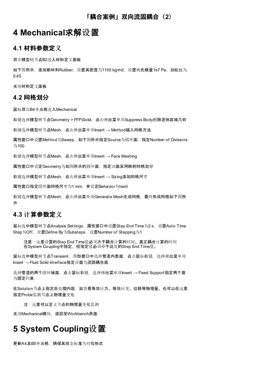
「耦合案例」双向流固耦合(2)4 Mechanical求解设置4.1 材料参数定义双击模型树节点B2进入材料定义面板如下图所示,添加新材料Rubber,设置其密度为1100 kg/m3,设置杨氏模量1e7 Pa,泊松比为0.45关闭材料定义面板4.2 网格划分鼠标双击B4单元格进入Mechanical右键选择模型树节点Geometry > FFF\Solid,点击弹出菜单项Suppress Body删除流体区域几何右键选择模型树节点Mesh,点击弹出菜单项Insert → Method插入网格方法属性窗口中设置Method为Sweep,如下图所示指定Source为圆环面,指定Number of Divisions 为100右键选择模型树节点Mesh,点击弹出菜单项Insert → Face Meshing属性窗口中设定Geometry为如图所示的圆环面,指定该面采用映射网格划分右键选择模型树节点Mesh,点击弹出菜单项Insert → Sizing添加网格尺寸属性窗口指定圆环面网格尺寸为1 mm,并设定Behavior为hard右键选择模型树节点Mesh,点击弹出菜单项Generate Mesh生成网格,最终形成网格如下图所示4.3 计算参数定义鼠标选中模型树节点Analysis Settings,属性窗口中设置Step End Time为2 s,设置Auto Time Step为Off,设置Define By为Substeps,设置Number of Stepping为1注意:这里设置的Step End Time值必须大于耦合计算的时间。
真正耦合计算的时间在System Coupling中指定,但指定值必须小于此处的Step End Time值。
鼠标选中模型树节点Transient,图形窗口中选择管道内表面,点击鼠标右键,选择弹出菜单项Insert → Fluid Solid Interface指定该面为流固耦合面选择管道的两个圆环端面,点击鼠标右键,选择弹出菜单项Insert → Fixed Support指定两个面为固定约束在Solution节点上指定后处理内容,如查看等效应力、等效应变、位移等物理量。
双向流固耦合和单向流固耦合
双向流固耦合和单向流固耦合说到流固耦合,可能你会觉得有点头大,这听起来像是工程师的专属术语,其实就是流体和固体相互“搅和”的故事。
简单来说,它指的就是流体的流动跟固体的形变之间的相互作用。
想象一下,河水冲击着堤坝,水流的速度和冲击力会影响堤坝的结构;而堤坝的强度和形状,又反过来影响水流的走向。
听起来是不是有点像是我们生活中两个人拉锯战的情形?没错,这就是“流固耦合”,流体和固体的互动,完全离不开彼此的“捆绑”!这时候,你可能会问:单向流固耦合和双向流固耦合到底有什么区别呢?简单说,单向流固耦合就好比是单方出击,水流影响固体,但固体对水流的影响几乎可以忽略不计。
就好比你和朋友一起走在路上,你一直往前走,朋友只是跟着你跑,不会影响到你前进的速度。
就像飞行器在大气中飞行,空气流动影响机翼的形状,但机翼对空气流动几乎没有影响。
简单明了,没什么复杂的交互。
而双向流固耦合就不一样了!它更像是两个人在一起跳舞,谁也不敢停下脚步,彼此影响,彼此反应。
想象一下你在舞池中跳舞,不仅要考虑自己的动作,还得时刻注意舞伴的反应。
比如,空气流动影响到飞机的机翼形态,而机翼的变化又影响到气流的变化,气流的变化又反过来影响机翼的形状。
这可不是简单的“你走你的,我走我的”,是相互依存、互相影响的精密合作。
听着是不是挺复杂?其实这就像我们生活中的各种合作关系一样:大家都在一条船上,哪怕是一个小小的波动,也能影响到整个系统的稳定。
为什么这两者的区分很重要呢?因为在很多实际问题中,搞清楚是单向的影响还是双向的互动,能帮助我们更好地解决问题。
如果是单向耦合,那就简简单单地解决问题就行,计算量小,模型简单,没啥难度;但是一旦是双向流固耦合,那可就得复杂多了。
你得同时考虑到固体和流体的影响,甚至还要考虑到它们之间的反馈作用,这就让问题变得非常有挑战性。
毕竟,不是每个人都喜欢做那种需要两头都照顾的事情吧?但这里的挑战并不意味着无解!如今的科学家们早就用计算机技术帮我们解决了大部分的难题。
CFX_流固双向耦合的实现
CFX_流固双向耦合的实现实现流固双向耦合需要以下几个步骤:1. 网格生成:首先需要生成流体和固体模型的网格。
对于流体,可以使用常规的CFD网格生成软件(如Ansys ICEM-CFD)生成适当的流体网格。
对于固体,可以使用CAD软件生成固体模型,并通过网格生成软件(如Ansys Meshing)将其转换为固体网格。
2. 物理模型设定:根据实际情况,选择合适的流体和固体模型进行设定。
对于流体,可以选择使用Navier-Stokes方程来描述流体的运动。
对于固体,可以选择使用弹性力学方程进行模拟。
3.边界条件设定:对于流体和固体的边界条件进行设定。
对于流体,包括入口流速、出口压力、壁面摩擦等边界条件。
对于固体,包括固体的位移、力或者应力等边界条件。
4. 数值求解:根据设定的物理模型和边界条件,使用CFX软件进行数值求解。
CFX使用有限体积法对Navier-Stokes方程进行离散化,同时使用显式或隐式方法求解弹性力学方程。
5.耦合求解:在流固双向耦合中,流体和固体之间的相互作用需要通过迭代的方式求解。
首先,在给定流体的边界条件下,使用CFX求解流体部分的问题。
然后,在给定固体的边界条件下,使用CFX求解固体部分的问题。
接着,将固体的变形信息传递给流体,影响流体的边界条件。
再次使用CFX求解流体的问题,得到新的流场分布。
重复这个过程,直到流体和固体的解收敛。
6.结果分析:对求解得到的结果进行分析和后处理。
可以通过CFX提供的后处理工具,如应力和变形分布、速度和压力分布等来评估流固耦合模拟的效果。
值得注意的是,流固双向耦合模拟的实现通常需要较高的计算资源和时间。
同时,由于流固耦合问题的复杂性,对物理模型的设定以及边界条件的设定也需要经验和专业知识。
综上所述,CFX流固双向耦合的实现可以分为网格生成、物理模型设定、边界条件设定、数值求解、耦合求解和结果分析等几个步骤。
通过迭代的方式求解流固双向耦合问题,可以模拟流体和固体之间的相互作用,为工程实践提供有价值的参考。
(整理)FLUENT14双向流固耦合案例.
说明:本例只应用于FLUENT14.0以上版本。
ANSYS 14.0是2011年底新推出的版本,在该版本中,加入了一个新的模块System Coupling,目前只能用于fluent与ansys mechanical的双向流固耦合计算。
官方文档中有介绍说以后会逐渐添加对其它求解器的支持,不过这不重要,重要的是现在FLUENT终于可以不用借助第三方软件进行双向流固耦合计算了,个人认为这是新版本一个不小的改进。
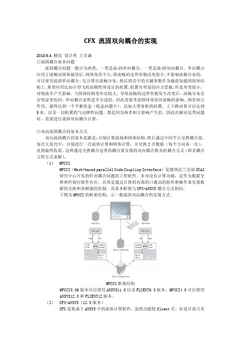
模块及数据传递方式如下图所示。
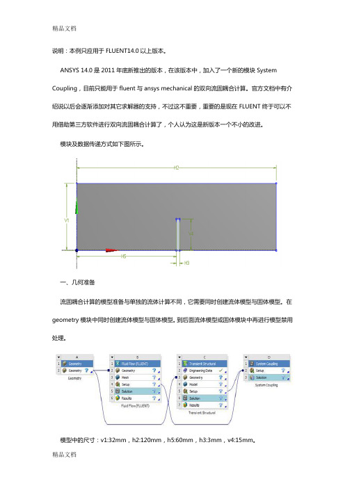
一、几何准备流固耦合计算的模型准备与单独的流体计算不同,它需要同时创建流体模型与固体模型。
在geometry模块中同时创建流体模型与固体模型。
到后面流体模型或固体模块中再进行模型禁用处理。
模型中的尺寸:v1:32mm,h2:120mm,h5:60mm,h3:3mm,v4:15mm。
由于流体计算中需要进行动网格设置,因此推荐使用四面体网格。
当然如果挡板刚度很大网格变形很小时,可以使用六面体网格,划分六面体网格可以先将几何进行slice切割。
这里对流体区域网格划分六面体网格,固体域同样划分六面体网格。
二、流体部分设置1、网格划分双击B3单元格,进入meshing模块进行网格划分。
禁用固体部分几何。
设定各相关部分的尺寸,由于固体区域几何较为整齐,因此在切割后只需设定一个全局尺寸即可划分全六面体网格。
这里设定全局尺寸为1mm。
划分网格后如下图所示。
2、进行边界命名,以方便在fluent中进行边界条件设置设置左侧面为速度进口velocity inlet,右侧面为自由出流outflow,上侧面为壁面边界wall_top,正对的两侧面为壁面边界wall_side1与wall_side2(这两个边界在动网格设定中为变形域),设定与固体交界面为壁面边界(该边界在动网格中设定为system coupling类型)。
操作方式:选择对应的表面,点击右键,选择菜单create named selection,然后输入相应的边界名称。
CFX_流固双向耦合的实现
CFX 流固双向耦合的实现2010.6.4 精仪 设计所 王昊森○流固耦合基本问题流固耦合问题一般分为两类,一类是流‐固单向耦合,一类是流‐固双向耦合。
单向耦合应用于流畅对固体最用后,固体变形不大,即流畅的边界形貌改变很小,不影响流畅分布的,可以使用流固单向耦合。
先计算出流畅分布,然后将其中的关键参数作为载荷加载到固体结构上。
典型应用比如小型飞机按刚性体设计的机翼,机翼有明显的应力受载,但是形变很小,对绕流不产生影响。
当固体结构变形比较大,导致流畅的边界形貌发生改变后,流畅分布会有明显变化时,单向耦合显然是不合适的,因此需要考虑固体变形对流畅的影响。
两者相互作用,最终达到一个平衡状态(稳态问题中)。
比如大型客机的机翼,上下跳动量可以达到5米,以及一切机翼的气动弹性问题,都是因为两者相互影响产生的。
因此在解决这类问题时,需要进行流固双向耦合计算。
○双向流固耦合的基本方式双向流固耦合的基本思路是:分别计算流场和固体结构,然后通过中间平台交换耦合量。
每次大迭代中,分别进行一次流体计算和固体计算,并交换2次数据(每个方向各一次),直到最终收敛。
这种通过交换耦合边界的耦合量实现的双向耦合称为松耦合方式(即非耦合方程方式求解)。
(1) MPCCIMPCCI(Mesh-based parallel Code Coupling Interface)是德国法兰克福SCAI研究中心开发的针对耦合问题的工程软件。
本身没有计算功能,是作为数据交换和控制台软件存在。
具体是通过计算机内部的口通讯的监听和操作来实现数据的交换和求解器的控制。
其基本框架与CFX-ANSYS耦合方式相同。
下图为MPCCI的框架结构,示一般流固双向耦合的实现方式。
MPCCI框架结构MPCCI3.06版本可以使用ANSYS11.0以及FLUENT6.3版本。
MPCCI4.0可以使用ANSYS12.0和FLUENT12版本。
(2) CFX-ANSYS(12.0版本)CFX是集成于ANSYS中的流体计算软件,虽然功能较fluent差,但是目前只有CFX可以不借助第三方软件与ANSYS实现双向流固耦合的计算。
fluent流固耦合案例
fluent流固耦合案例
一个常见的流固耦合案例是风洞实验。
风洞是一个用于模拟飞行器在风场中运动的设备,其中飞行器模型放置在流场中,通过控制风洞内的气流运动来模拟不同飞行状态下的飞行器性能。
在风洞实验中,流体(空气)和固体(飞行器模型)之间存在耦合关系。
流体流动会受到飞行器模型的阻力、升力等力的影响,同时飞行器模型的形状、表面特性也会影响流体的流动状态。
通过调整风洞中的气流速度、飞行器模型的姿态等参数,可以模拟不同飞行状态下的流体流动和飞行器性能,帮助工程师评估飞行器设计的稳定性、升阻比、气动特性等。
在这个案例中,流体和固体之间的流固耦合是通过相互作用来实现的。
流体的速度和压力分布会受到固体表面的细微变化影响,而固体的运动和力学性能则会受到流体的作用力和流动状况的限制。
通过对风洞实验的观测和数据分析,可以获取关于飞行器在不同飞行状态下的气动性能的重要信息,为改进飞行器设计、提高性能和安全性提供参考。
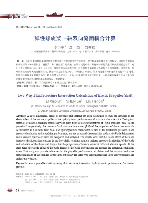
弹性螺旋桨-轴双向流固耦合计算
31、别人笑我太疯癫,我笑他人看不 穿。(名 言网) 32、我不想听失意者的哭泣,抱怨者 的牢骚 ,这是 羊群中 的瘟疫 ,我不 能被它 传染。 我要尽 量避免 绝望, 辛勤耕 耘,忍 受苦楚 。我一 试再试 ,争取 每天的 成功, 避免以 失败收 常在别 人停滞 不怕前面跌宕的山岩,生命 就永远 只能是 死水一 潭。 34、当你眼泪忍不住要流出来的时候 ,睁大 眼睛, 千万别 眨眼!你会看到 世界由 清晰变 模糊的 全过程 ,心会 在你泪 水落下 的那一 刻变得 清澈明 晰。盐 。注定 要融化 的,也 许是用 眼泪的 方式。
35、不要以为自己成功一次就可以了 ,也不 要以为 过去的 光荣可 以被永 远肯定 。
谢谢你的阅读
❖ 知识就是财富 ❖ 丰富你的人生
71、既然我已经踏上这条道路,那么,任何东西都不应妨碍我沿着这条路走下去。——康德 72、家庭成为快乐的种子在外也不致成为障碍物但在旅行之际却是夜间的伴侣。——西塞罗 73、坚持意志伟大的事业需要始终不渝的精神。——伏尔泰 74、路漫漫其修道远,吾将上下而求索。——屈原 75、内外相应,言行相称。——韩非
- 1、下载文档前请自行甄别文档内容的完整性,平台不提供额外的编辑、内容补充、找答案等附加服务。
- 2、"仅部分预览"的文档,不可在线预览部分如存在完整性等问题,可反馈申请退款(可完整预览的文档不适用该条件!)。
- 3、如文档侵犯您的权益,请联系客服反馈,我们会尽快为您处理(人工客服工作时间:9:00-18:30)。
双向流固耦合实例(Fluent与structure)
说明:本例只应用于FLUENT14.0以上版本。
ANSYS 14.0是2011年底新推出的版本,在该版本中,加入了一个新的模块System Coupling,目前只能用于fluent与ansys mechanical的双向流固耦合计算。
官方文档中有介绍说以后会逐渐添加对其它求解器的支持,不过这不重要,重要的是现在FLUENT终于可以不用借助第三方软件进行双向流固耦合计算了,个人认为这是新版本一个不小的改进。
模块及数据传递方式如下图所示。
一、几何准备
流固耦合计算的模型准备与单独的流体计算不同,它需要同时创建流体模型与固体模型。
在geometry模块中同时创建流体模型与固体模型。
到后面流体模型或固体模块中再进行模型禁用处理。
模型中的尺寸:v1:32mm,h2:120mm,h5:60mm,h3:3mm,v4:15mm。
由于流体计算中需要进行动网格设置,因此推荐使用四面体网格。
当然如果挡板刚度很大网格变形很小时,可以使用六面体网格,划分六面体网格可以先将几何进行slice切割。
这里对流体区域网格划分六面体网格,固体域同样划分六面体网格。
二、流体部分设置
1、网格划分
双击B3单元格,进入meshing模块进行网格划分。
禁用固体部分几何。
设定各相关部分的尺寸,由于固体区域几何较为整齐,因此在切割后只需设定一个全局尺寸即可划分全六面体网格。
这里设定全局尺寸为1mm。
划分网格后如下图所示。
2、进行边界命名,以方便在fluent中进行边界条件设置
设置左侧面为速度进口velocity inlet,右侧面为自由出流outflow,上侧面为壁面边界wall_top,正对的两侧面为壁面边界wall_side1与wall_side2(这两个边界在动网格设定中为变形域),设定与固体交界面为壁面边界(该边界在动网格中设定为system coupling类型)。
操作方式:选择对应的表面,点击右键,选择菜单create named selection,然后输入相应的边界名称。
注意:FLUENT会自动检测输入的名称以使用对应的边界类型,当然用户也可以在fluent进行类型更改。
完成后的树形菜单如下图所示。
本部分操作完毕后,关闭meshing模块。
返回工程面板。
3、进入fluent设置
FLUENT主要进行动网格设置。
其它设置与单独进行FLUENT仿真完全一致。
设置使用瞬态计算,使用K-Epsilon湍流模型。
这里的动网格主要使用弹簧光顺处理(由于使用的是六面体网格且运动不规律),需要使用TUI命令打开光顺对六面体网格的支持。
使用命令
/define/dynamic-mesh/controls/smoothing-parameters。
动态层技术与网格重构方法在六面体网格中失效。
因此,建议使用四面体网格。
我们这里由于变形小,所以只使用光顺方法即可满足要求。
点击Dynamic mesh进入动网格设置面板。
如下图所示,激活动网格模型。
4、smoothing参数
使用弹簧光顺方法。
设置参数弹簧常数0.6,边界节点松弛因子0.6。
如下图所示。
5、运动区域设置
主要包括三个运动区域:流固耦合面、两侧的面。
其中流固耦合面运动方式为system coupling,两侧壁面运动类型为deforming。
设置最小网格尺寸0.8,最大网格尺寸1.5,最大扭曲率0.6。
如下图所示(点击查看大图)。
6、其它设置
包括求解控制参数设置、动画设置、自动保存设置、初始化设置、计算时间步及步长设置等。
与单独FLUENT使用没有任何差异。
迭代参数设置如下图所示。
关闭FLUENT,返回工程面板。
二、固体部分设置
1、材料设置
双击C2单元格进入固体材料设置。
这里保持默认的结构钢。
弹性模量2.1e11Pa,泊松比0.3。
需要注意的是材料特性决定了变形,因此对于刚度小的材料可能会存在大的位移,在流体求解器中动网格设置时需要加以关注。
点击retrun to project回到工程面板。
2、网格划分及进行约束
双击C4单元格进入固体网格划分模块。
设定网格尺寸1mm划分网格。
添加流固耦合面及固定边界约束。
设置分析参数,时间步长设置为0.01s,总时间为1s。
如下图所示。
设置完毕后,关闭DS返回工程面板。
右键单击C5单元格,选择update进行更新。
三、System Coupling设置
1、设置时间耦合
双击D2单元格,进入System Coupling面板。
点击Analysis Settings,如左下图所示。
在弹出的面板中设置end time为1s,设置step size为0.01s,如右上图所示。
2、设置耦合面
点选ctrl的同时选择固体与流体中的耦合面名称,点击右键,创建流固耦合面。
如下图所示。
点击Co-Sim. sequence单元格,在弹出的编辑面板中设置各求解器的启动顺序。
设置fluent为1,Transient为2。
如下图所示。
3、进行流固耦合计算
通过点击工具栏上的Update Project按钮进行流固耦合计算。