Matlab代码1运行结果
MATLAB实验代码与运行结果
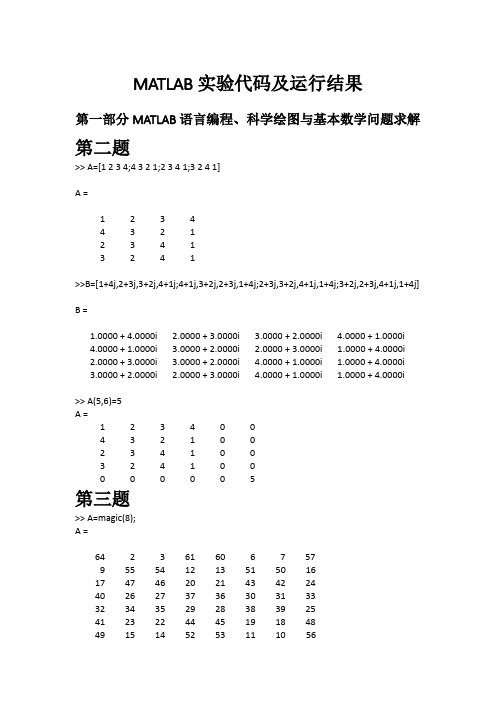
MATLAB实验代码及运行结果第一部分MATLAB语言编程、科学绘图与基本数学问题求解第二题>> A=[1 2 3 4;4 3 2 1;2 3 4 1;3 2 4 1]A =1 2 3 44 3 2 12 3 4 13 24 1>>B=[1+4j,2+3j,3+2j,4+1j;4+1j,3+2j,2+3j,1+4j;2+3j,3+2j,4+1j,1+4j;3+2j,2+3j,4+1j,1+4j]B =1.0000 + 4.0000i2.0000 +3.0000i 3.0000 + 2.0000i4.0000 + 1.0000i4.0000 + 1.0000i 3.0000 + 2.0000i 2.0000 + 3.0000i 1.0000 + 4.0000i2.0000 +3.0000i 3.0000 + 2.0000i4.0000 + 1.0000i 1.0000 + 4.0000i3.0000 + 2.0000i 2.0000 + 3.0000i4.0000 + 1.0000i 1.0000 + 4.0000i >> A(5,6)=5A =1 2 3 4 0 04 3 2 1 0 02 3 4 1 0 03 24 1 0 00 0 0 0 0 5第三题>> A=magic(8);A =64 2 3 61 60 6 7 579 55 54 12 13 51 50 1617 47 46 20 21 43 42 2440 26 27 37 36 30 31 3332 34 35 29 28 38 39 2541 23 22 44 45 19 18 4849 15 14 52 53 11 10 568 58 59 5 4 62 63 1 B=A(2:2:end,:)B =9 55 54 12 13 51 50 1640 26 27 37 36 30 31 3341 23 22 44 45 19 18 488 58 59 5 4 62 63 1 第四题>> format long;sum(2.^[0:63])ans =1.844674407370955e+19>> sum(sym(2).^[0:63])ans =18446744073709551615第五题(1)>> x=[-1:0.001:1];y=sin(1./x);plot(x,y)(2)>>t=[-pi:0.005:pi];y=sin(tan(t))-tan(sin(t));plot(t,y)第六题[x,y]=meshgrid(-2:0.1:2);z=1./(sqrt((1-x).^2+y.^2))+1./(sqrt((1+x).^2+y.^2));subplot(2 24),surf(x,y,z),shadingflat;subplot(221),surf(x,y,z),view(0,90);subplot(222),surf(x,y,z),view(90,0);subplot(22 3),surf(x,y,z),view(0,0)>>Warning: Divide by zero.Warning: Divide by zero.xx=[-2:0.1:-1.2,-1.1:0.02:-0.9,-0.8:0.1:0.8,0.9:0.02:1.1,1.2:0.1:2];yy=[-1:0.1:-0.2,-0.1:0 .02:0.1,0.2:0.1:1];[x,y]=meshgrid(xx,yy);z=1./((sqrt(1-x).^2+y.^2))+1./(sqrt((1+x).^2+y. ^2));subplot(224),surf(x,y,z),shadingflat;zlim([0,15]);subplot(221),surf(x,y,z),view(0,90);subplot(222),surf(x,y,z),view(90,0) ;subplot(223),surf(x,y,z),view(0,0)第七题(1)>> syms x;f=(3^x+9^x)^(1/x);limit(f,x,inf)ans =9(2)>> syms x y;f=x*y/(sqrt(x*y+1)-1);limit(limit(f,y,0),x,0)ans =2(3)>> syms x y;f=(1-cos(x^2+y^2))/((x^2+y^2)*exp(x^2+y^2));limit(limit(f,y,0),x,0) ans =第八题第一步新建脚本function result=paradiff(y,x,t,n)if mod(n,1)~=0,error('n should positive innteger,please correct')else if n==1,result=diff(y,t)/diff(x,t);else result=diff(y,x,t,n-1)/diff(x,t);end,end(1)syms t;x=log(cos(t));y=cos(t)-t*sin(t);f=simplify(paradiff(y,x,t,1))f =(cos(t)*(2*sin(t) + t*cos(t)))/sin(t)(2)syms t;f=(cos(t)*(2*sin(t) + t*cos(t)))/sin(t);f1=diff(f)f1 =(cos(t)*(3*cos(t) - t*sin(t)))/sin(t) - t*cos(t) - (cos(t)^2*(2*sin(t) + t*cos(t)))/sin(t)^2 - 2*sin(t)t=pi/3;f1 =(cos(t)*(3*cos(t) - t*sin(t)))/sin(t) - t*cos(t) - (cos(t)^2*(2*sin(t) + t*cos(t)))/sin(t)^2 - 2*sin(t)f1 =-2.6651第九题>> syms x y t;f=int(exp(-t^2),t,0,x*y);F=(x/y)*(diff(f,x,2))-2*(diff(diff(f,x,1),y,1))+diff(f,y,2)F =2*x^2*y^2*exp(-x^2*y^2) - 2*x^3*y*exp(-x^2*y^2) - 2*exp(-x^2*y^2)第十题(1)>> syms n m;limit(symsum(1/((2*m)^2-1),m,1,n),n,inf)1/2(2)>> syms m n;limit(symsum(n*(1/(n^2+m*pi)),m,1,n),n,inf)ans =1第十一题(1)>> syms t;syms a positive;x=a*(cos(t)+t*sin(t));y=a*(sin(t)-t*cos(t));I=int((x^2+y^2)*sqrt(diff(y,t)^2+diff (x,t)^2),t,0,2*pi)I =2*pi^2*a^3*(2*pi^2 + 1)(2)>> syms t x y;syms a c b positive;x=c*cos(t)/a;y=c*sin(t)/b;F=[y*x^3+exp(y),x*y^3+x*exp(y)-2*y];ds=[diff(x,t); diff(y,t)]; I=int(F*ds,t,pi,0)I =(2*c*(15*b^4 - 2*c^4))/(15*a*b^4)第十二题>> syms a b c d e;A=[a^4,a^3,a^2,a,1;b^4,b^3,b^2,b,1;c^4,c^3,c^2,c,1;d^4,d^3,d^2,d,1;e^4,e^3,e^2,e,1];simplify (det(A))ans =(a - b)*(a - c)*(a - d)*(b - c)*(a - e)*(b - d)*(b - e)*(c - d)*(c - e)*(d - e)第十三题>> A=[2 0.5 -0.5 0.5;0 -1.5 0.5 -0.5;2,0.5 -4.5 0.5;2 1 -2 -2];[V,J]=jordan(sym(A))V =[ 0, 1/8, 1/2, 3/8][ 0, 0, -2, -3][ -1/6, 1/24, -1/2, 1/8][ -1/6, 1/24, -5/2, 9/8]J =[ -4, 0, 0, 0][ 0, 2, 0, 0][ 0, 0, -2, 1][ 0, 0, 0, -2]第十四题编写函数代码function X=lyapsym(A,B,C)if nargin==2,C=B;B=A';end[nr,nc]=size(C);A0=kron(A,eye(nc))+kron(eye(nr),B');tryC1=C';x0=-inv(A0)*C1(:);X=reshape(x0,nc,nr)';catch,error('singular matrix found.'),end>> A=[3 -6 -4 0 5;1 4 2 -2 4;-6 3 -6 7 3;-13 10 0 -11 0;0 4 0 3 4];B=[3 -2 1;-2 -9 2;-2 -1 9];C=-[-2 1 -1;4 1 2;5 -6 1;6 -4 -4;-6 6 -3];X=lyap(A,B,C),norm(A*X+X*B+C);X=lyapsym(sym(A),B,C),norm(A*X+X*B+C)X =4.0569 14.5128 -1.5653-0.0356 -25.0743 2.7408-9.4886 -25.9323 4.4177-2.6969 -21.6450 2.8851-7.7229 -31.9100 3.7634X =[ 434641749950/107136516451, 4664546747350/321409549353, -503105815912/321409549353][ -3809507498/107136516451, -8059112319373/321409549353, 880921527508/321409549353][ -1016580400173/107136516451, -8334897743767/321409549353, 1419901706449/321409549353][ -288938859984/107136516451, -6956912657222/321409549353, 927293592476/321409549353][ -827401644798/107136516451, -10256166034813/321409549353, 1209595497577/321409549353](2)>> A=[3 -6 -4 0 5;1 4 2 -2 4;-6 3 -6 7 3;-13 10 0 -11 0;0 4 0 3 4];B=[3 -2 1;-2 -9 2;-2 -1 9];C=-[-2 1 -1;4 1 2;5 -6 1;6 -4 -4;-6 6 -3];X=lyap(A,B,C),norm(A*X+X*B+C)X =4.0569 14.5128 -1.5653-0.0356 -25.0743 2.7408-9.4886 -25.9323 4.4177-2.6969 -21.6450 2.8851-7.7229 -31.9100 3.7634ans =3.4356e-13第十五题>> syms t;A=[-4.5,0,0.5,-1.5;-0.5,-4,0.5,-0.5;1.5,1,-2.5,1.5;0,-1,-1,-3];B=simplify(expm(A*t))B =[ (exp(-5*t)*(exp(2*t) - t*exp(2*t) + t^2*exp(2*t) + 1))/2, (exp(-5*t)*(2*t*exp(2*t) - exp(2*t) + 1))/2, (t*exp(-3*t)*(t + 1))/2, -(exp(-5*t)*(exp(2*t) + t*exp(2*t) - t^2*exp(2*t) - 1))/2][ (exp(-5*t)*(t*exp(2*t) - exp(2*t) + 1))/2, (exp(-5*t)*(exp(2*t) + 1))/2, (t*exp(-3*t))/2, (exp(-5*t)*(t*exp(2*t) - exp(2*t) + 1))/2][ (exp(-5*t)*(exp(2*t) + t*exp(2*t) - 1))/2, (exp(-5*t)*(exp(2*t) - 1))/2, (exp(-3*t)*(t + 2))/2, (exp(-5*t)*(exp(2*t) + t*exp(2*t) - 1))/2][ -(t^2*exp(-3*t))/2, -t*exp(-3*t), -(t*exp(-3*t)*(t + 2))/2, -(exp(-3*t)*(t^2 - 2))/2]>> C=simplify(sin(A*t))C =[ -sin((9*t)/2), 0, sin(t/2), -sin((3*t)/2)][ -sin(t/2), -sin(4*t), sin(t/2), -sin(t/2)][ sin((3*t)/2), sin(t), -sin((5*t)/2), sin((3*t)/2)][ 0, -sin(t), -sin(t), -sin(3*t)]>> D=simplify(expm(A*t)*sin(A^2*expm(A*t)*t))D =[ (exp(-5*t)*sin((t*exp(-5*t)*(9*t*exp(2*t) - 15*exp(2*t) + 25))/2)*(2*t*exp(2*t) - exp(2*t) + 1))/2 + (exp(-5*t)*sin((t*exp(-3*t)*(9*t^2 - 12*t + 2))/2)*(exp(2*t) + t*exp(2*t) - t^2*exp(2*t) - 1))/2 + (exp(-5*t)*sin((t*exp(-5*t)*(17*exp(2*t) - 21*t*exp(2*t) + 9*t^2*exp(2*t) + 25))/2)*(exp(2*t) - t*exp(2*t) + t^2*exp(2*t) + 1))/2 + (t*exp(-3*t)*sin((t*exp(-5*t)*(3*exp(2*t) + 9*t*exp(2*t) - 25))/2)*(t + 1))/2, (exp(-5*t)*sin((t*exp(-5*t)*(9*exp(2*t) + 25))/2)*(2*t*exp(2*t) - exp(2*t) + 1))/2 + (exp(-5*t)*sin((t*exp(-5*t)*(18*t*exp(2*t) - 21*exp(2*t) + 25))/2)*(exp(2*t) - t*exp(2*t) + t^2*exp(2*t) + 1))/2 + (exp(-5*t)*sin(3*t*exp(-3*t)*(3*t - 2))*(exp(2*t) + t*exp(2*t) - t^2*exp(2*t) - 1))/2 + (t*exp(-3*t)*sin((t*exp(-5*t)*(9*exp(2*t) - 25))/2)*(t + 1))/2, (exp(-5*t)*sin((3*t*exp(-3*t)*(3*t - 2))/2)*(2*t*exp(2*t) - exp(2*t) + 1))/2 - (exp(-5*t)*sin((t*exp(-3*t)*(- 9*t^2 + 3*t + 4))/2)*(exp(2*t) - t*exp(2*t) + t^2*exp(2*t) + 1))/2 + (exp(-5*t)*sin((t*exp(-3*t)*(9*t^2 + 6*t - 10))/2)*(exp(2*t) + t*exp(2*t) - t^2*exp(2*t) - 1))/2 + (t*exp(-3*t)*sin((3*t*exp(-3*t)*(3*t + 4))/2)*(t + 1))/2, (exp(-5*t)*sin((t*exp(-5*t)*(9*t*exp(2*t) - 15*exp(2*t) + 25))/2)*(2*t*exp(2*t) - exp(2*t) + 1))/2 - (exp(-5*t)*sin((t*exp(-5*t)*(exp(2*t) + 21*t*exp(2*t) - 9*t^2*exp(2*t) - 25))/2)*(exp(2*t) - t*exp(2*t) + t^2*exp(2*t) + 1))/2 - (exp(-5*t)*sin((t*exp(-3*t)*(- 9*t^2 + 12*t + 16))/2)*(exp(2*t) + t*exp(2*t) - t^2*exp(2*t) - 1))/2 + (t*exp(-3*t)*sin((t*exp(-5*t)*(3*exp(2*t) + 9*t*exp(2*t) - 25))/2)*(t + 1))/2][ (exp(-5*t)*sin((t*exp(-5*t)*(1 7*exp(2*t) - 21*t*exp(2*t) + 9*t^2*exp(2*t) + 25))/2)*(t*exp(2*t) - exp(2*t) + 1))/2 - (exp(-5*t)*sin((t*exp(-3*t)*(9*t^2 - 12*t + 2))/2)*(t*exp(2*t) - exp(2*t) + 1))/2 + (t*exp(-3*t)*sin((t*exp(-5*t)*(3*exp(2*t) + 9*t*exp(2*t) - 25))/2))/2 + (exp(-5*t)*sin((t*exp(-5*t)*(9*t*exp(2*t) - 15*exp(2*t) + 25))/2)*(exp(2*t) + 1))/2, (exp(-5*t)*sin((t*exp(-5*t)*(18*t*exp(2*t) - 21*exp(2*t) + 25))/2)*(t*exp(2*t) - exp(2*t) + 1))/2 - (exp(-5*t)*sin(3*t*exp(-3*t)*(3*t - 2))*(t*exp(2*t) - exp(2*t) + 1))/2 + (t*exp(-3*t)*sin((t*exp(-5*t)*(9*exp(2*t) - 25))/2))/2 + (exp(-5*t)*sin((t*exp(-5*t)*(9*exp(2*t) + 25))/2)*(exp(2*t) + 1))/2, (exp(-3*t)*sin((3*t*exp(-3*t)*(3*t - 2))/2))/2 + (exp(-5*t)*sin((3*t*exp(-3*t)*(3*t - 2))/2))/2 + (exp(-3*t)*sin((t*exp(-3*t)*(- 9*t^2 + 3*t + 4))/2))/2 - (exp(-5*t)*sin((t*exp(-3*t)*(- 9*t^2 + 3*t + 4))/2))/2 + (exp(-3*t)*sin((t*exp(-3*t)*(9*t^2 + 6*t - 10))/2))/2 - (exp(-5*t)*sin((t*exp(-3*t)*(9*t^2 + 6*t - 10))/2))/2 + (t*exp(-3*t)*sin((3*t*exp(-3*t)*(3*t + 4))/2))/2 - (t*exp(-3*t)*sin((t*exp(-3*t)*(- 9*t^2 + 3*t + 4))/2))/2 - (t*exp(-3*t)*sin((t*exp(-3*t)*(9*t^2 + 6*t - 10))/2))/2, (exp(-5*t)*sin((t*exp(-3*t)*(- 9*t^2 + 12*t + 16))/2)*(t*exp(2*t) - exp(2*t) + 1))/2 - (exp(-5*t)*sin((t*exp(-5*t)*(exp(2*t) + 21*t*exp(2*t) - 9*t^2*exp(2*t) - 25))/2)*(t*exp(2*t) - exp(2*t) + 1))/2 + (t*exp(-3*t)*sin((t*exp(-5*t)*(3*exp(2*t) + 9*t*exp(2*t) - 25))/2))/2 + (exp(-5*t)*sin((t*exp(-5*t)*(9*t*exp(2*t) - 15*exp(2*t) + 25))/2)*(exp(2*t) + 1))/2][ (exp(-5*t)*sin((t*exp(-5*t)*(17*ex p(2*t) - 21*t*exp(2*t) + 9*t^2*exp(2*t) + 25))/2)*(exp(2*t) + t*exp(2*t) - 1))/2 - (exp(-5*t)*sin((t*exp(-3*t)*(9*t^2 - 12*t + 2))/2)*(exp(2*t) + t*exp(2*t) - 1))/2 + exp(-3*t)*sin((t*exp(-5*t)*(3*exp(2*t) + 9*t*exp(2*t) - 25))/2)*(t/2 + 1) + (exp(-5*t)*sin((t*exp(-5*t)*(9*t*exp(2*t) - 15*exp(2*t) + 25))/2)*(exp(2*t) - 1))/2, exp(-3*t)*sin((t*exp(-5*t)*(9*exp(2*t) - 25))/2)*(t/2 + 1) + (exp(-5*t)*sin((t*exp(-5*t)*(9*exp(2*t) + 25))/2)*(exp(2*t) - 1))/2 + (exp(-5*t)*sin((t*exp(-5*t)*(18*t*exp(2*t) - 21*exp(2*t) + 25))/2)*(exp(2*t) + t*exp(2*t) - 1))/2 - (exp(-5*t)*sin(3*t*exp(-3*t)*(3*t - 2))*(exp(2*t) + t*exp(2*t) - 1))/2, exp(-3*t)*sin((3*t*exp(-3*t)*(3*t + 4))/2)*(t/2 + 1) - (exp(-5*t)*sin((t*exp(-3*t)*(9*t^2 + 6*t - 10))/2)*(exp(2*t) + t*exp(2*t) - 1))/2 - (exp(-5*t)*sin((t*exp(-3*t)*(- 9*t^2 + 3*t + 4))/2)*(exp(2*t) + t*exp(2*t) - 1))/2 + (exp(-5*t)*sin((3*t*exp(-3*t)*(3*t - 2))/2)*(exp(2*t) - 1))/2, (exp(-5*t)*sin((t*exp(-3*t)*(- 9*t^2 + 12*t + 16))/2)*(exp(2*t) + t*exp(2*t) - 1))/2 + exp(-3*t)*sin((t*exp(-5*t)*(3*exp(2*t) + 9*t*exp(2*t) - 25))/2)*(t/2 + 1) + (exp(-5*t)*sin((t*exp(-5*t)*(9*t*exp(2*t) - 15*exp(2*t) + 25))/2)*(exp(2*t) - 1))/2 - (exp(-5*t)*sin((t*exp(-5*t)*(exp(2*t) + 21*t*exp(2*t) - 9*t^2*exp(2*t) - 25))/2)*(exp(2*t) + t*exp(2*t) - 1))/2][exp(-3*t)*sin((t*exp(-3*t)*(9*t^2 - 12*t + 2))/2)*(t^2/2 - 1) - (t^2*exp(-3*t)*sin((t*exp(-5*t)*(17*exp(2*t) - 21*t*exp(2*t) + 9*t^2*exp(2*t) + 25))/2))/2 - t*exp(-3*t)*sin((t*exp(-5*t)*(9*t*exp(2*t) - 15*exp(2*t) + 25))/2) - (t*exp(-3*t)*sin((t*exp(-5*t)*(3*exp(2*t) + 9*t*exp(2*t) - 25))/2)*(t + 2))/2, exp(-3*t)*sin(3*t*exp(-3*t)*(3*t - 2))*(t^2/2 - 1) - t*exp(-3*t)*sin((t*exp(-5*t)*(9*exp(2*t) + 25))/2) - (t^2*exp(-3*t)*sin((t*exp(-5*t)*(18*t*exp(2*t) - 21*exp(2*t) + 25))/2))/2 - (t*exp(-3*t)*sin((t*exp(-5*t)*(9*exp(2*t) - 25))/2)*(t + 2))/2, -(exp(-3*t)*(2*sin((t*exp(-3*t)*(9*t^2 + 6*t - 10))/2) - t^2*sin((t*exp(-3*t)*(- 9*t^2 + 3*t + 4))/2) - t^2*sin((t*exp(-3*t)*(9*t^2 + 6*t - 10))/2) + 2*t*sin((3*t*exp(-3*t)*(3*t - 2))/2) + 2*t*sin((3*t*exp(-3*t)*(3*t + 4))/2) + t^2*sin((3*t*exp(-3*t)*(3*t + 4))/2)))/2, exp(-3*t)*sin((t*exp(-3*t)*(- 9*t^2 + 12*t + 16))/2) - (t^2*exp(-3*t)*sin((t*exp(-3*t)*(- 9*t^2 + 12*t + 16))/2))/2 - t*exp(-3*t)*sin((t*exp(-5*t)*(3*exp(2*t) + 9*t*exp(2*t) - 25))/2) - t*exp(-3*t)*sin((t*exp(-5*t)*(9*t*exp(2*t) - 15*exp(2*t) + 25))/2) - (t^2*exp(-3*t)*sin((t*exp(-5*t)*(3*exp(2*t) + 9*t*exp(2*t) - 25))/2))/2 + (t^2*exp(-3*t)*sin((t*exp(-5*t)*(exp(2*t) + 21*t*exp(2*t) - 9*t^2*exp(2*t) - 25))/2))/2]第二部分数学问题求解与数据处理第一题(1)>> syms a t;f=sin(a*t)/t;F=simplify(laplace(f))F =atan(a/s)(2)>> syms a t;f=t^5*sin(a*t);F=simplify(laplace(f))F =(240*a*s*(3*a^4 - 10*a^2*s^2 + 3*s^4))/(a^2 + s^2)^6(3)>> syms a t;f=t^8*cos(a*t);F=simplify(laplace(f))F =(40320*s*(9*a^8 - 84*a^6*s^2 + 126*a^4*s^4 - 36*a^2*s^6 + s^8))/(a^2 + s^2)^9 第二题(1)>> syms a s b t;f=1/(sqrt(s*s)*(s^2-a^2)*(s+b));f1=ilaplace(f,s,t)f1 =-ilaplace(1/((b + s)*(a^2 - s^2)*(s^2)^(1/2)), s, t)(2)>> syms s a b t;f=sqrt(s-a)-sqrt(s-b);f1=ilaplace(f,s,t)f1 =ilaplace((s - a)^(1/2), s, t) - ilaplace((s - b)^(1/2), s, t)(3)>> syms a b s t;f=log((s-a)/(s-b));f1=ilaplace(f,s,t)f1 =exp(b*t)/t - exp(a*t)/t第三题(1)>> syms x t;f=x^2*(3*pi-abs(2*x));f1=ifourier(f,x)f1 =-(24/x^4 + 6*pi^2*dirac(x, 2))/(2*pi)(2)>> syms t;f=t^2*(t-2*pi);f1=ifourier(f,t)f1 =(pi*dirac(t, 3)*2*i + 4*pi^2*dirac(t, 2))/(2*pi)第四题(1)>> syms a T K;f=cos(K*a*T);f1=ztrans(f);f2=iztrans(f1)f2 =cos(K*T*n)(2)>> syms a T K;f=(K*T)^2*exp(-a*K*T);f1=ztrans(f);f2=iztrans(f1)f2 =K^2*T^2*kroneckerDelta(n, 0) - K^2*T^2*exp(-K*T)*(exp(K*T)*kroneckerDelta(n, 0) - exp(-K*T)^n*exp(K*T))(3)>> syms a K T;f=(a*T*K-1+exp(-a*T*K))/a;f1=ztrans(f);f2=iztrans(f1)f2 =exp(-K*T)^n/n - 1/n - K*T*(kroneckerDelta(n, 0) - 1) + K*T*kroneckerDelta(n, 0)第五题(1)>> syms x;f=exp(-(x+1)^2+pi/2)*sin(5*x+2);t=solve(f)t =-2/5>> subs(f,x,-2/5)ans =(2)>> syms x y;f=(x^2+y^2+x*y)*exp(-x^2-y^2-x*y);x1=solve('(x^2+y^2+x*y)*exp(-x^2-y^2-x*y)','x') x1 =- y/2 + (3^(1/2)*y*i)/2- y/2 - (3^(1/2)*y*i)/2>> simplify(subs(f,x,x1))ans =第六题>> syms c x;solve(diff(int((exp(x)-c*x)^2,x,0,1),c))ans =3第七题写函数: function [c,ce]=c6exmcon(x)ce=[];c=[x(1)+x(2);x(1)*x(2)-x(1)-x(2)+1.5;-10-x(1)*x(2)];>> clear P;P.nonlcon=@c6exmcon;P.solver='fmincon';P.options=optimset;P.objective=@(x)exp(x(1))*(4*x( 1)^2+2*x(2)^2+4*x(1)*x(2)+2*x(2)+1);...ff=optimset;ff.TolX=1e-20;ff.TolFum=1e-20;P.options=ff;P.lb=[-10;-10];P.ub=-P.lb;P.x0=[0;0];[x,f1,fla g]=fmincon(P)Local minimum found that satisfies the constraints.Optimization completed because the objective function is non-decreasing infeasible directions, to within the default value of the function tolerance,and constraints are satisfied to within the default value of the constraint tolerance.<stopping criteria details>x =1.1825-1.7398f1 =3.0608flag =1第八题N=10;[x1,x2,x3,x4,x5,x6,x7]=ndgrid(1:N,1:N,4:N,1:N,2:N,5:N,6:N);i=find((-x1<=0)&(-x2<=0)&(-x3< =0)&(-x4<=0)&(-x5<=0)&(-x6<=0)&(-x7<=0)&(3534*x1+2356*x2+1767*x3+589*x4+528*x5+451* x6+304*x7<=119567));x1=x1(i);x2=x2(i);x3=x3(i);x4=x4(i);x5=x5(i);x6=x6(i);x7=x7(i);f=592*x1+381 *x2+273*x3+55*x4+48*x5+37*x6+23*x7;[fmax,ii]=sort(f);index=ii(1);x=[x1(index),x2(index),x3(in dex),x4(index),x5(index),x6(index),x7(index)]x =1 1 4 12 5 6第九题syms x y;y1=dsolve('D2y-(2-1/x)*Dy+(1-1/x)*y=x^2*exp(-5*x)','x');simplify(y1)ans =(exp(-5*x)*(30*x - 6*ei(-6*x)*exp(6*x) + 36*x^2 + 1296*C7*exp(6*x) + 1296*C8*exp(6*x)*log(x) + 11))/1296>> y=dsolve('D2y-(2-1/x)*Dy+(1-1/x)*y=x^2*exp(-5*x)','y(1)=sym(pi)','y((pi))=1','x');simplify(y)ans =(exp(-5*x)*(30*x + 6*log(x) + 108*x^2*log(x) + 216*x^3*log(x) - 6*ei(-6*x)*exp(6*x) + 36*x*log(x) + 36*x^2 + 11))/1296 - (exp(-5*x)*log(x)*(216*x^3 + 108*x^2 + 36*x + 6))/1296 + (exp(-6)*exp(x)*(6*ei(-6)*exp(6) + 1296*exp(5)*sym(pi) - 77))/1296 - (exp(-6*pi)*exp(-6)*exp(x)*log(x)*(11*exp(6) - 77*exp(6*pi) + 30*pi*exp(6) + 36*pi^2*exp(6) - 1296*exp(5*pi)*exp(6) + 6*ei(-6)*exp(6*pi)*exp(6) + 1296*exp(6*pi)*exp(5)*sym(pi) - 6*exp(6*pi)*exp(6)*ei(-6*pi)))/(1296*log(pi))第十题(1)>> syms t;x=dsolve('D2x+2*t*Dx+t^2*x=t+1');simplify(x)ans =C4*exp(-(t*(t - 2))/2) + C5*exp(-(t*(t + 2))/2) - (2^(1/2)*pi^(1/2)*erf(2^(1/2)*((t*i)/2 - i/2))*exp(-(t - 1)^2/2)*i)/2(2)>> syms x y;y=dsolve('Dy+2*x*y=x*exp(-x^2)')y =(exp(-x^2)*(C2*exp(-2*t*x) + 1))/2第十一题>>f=@(t,x)[-x(2)-x(3);x(1)+0.2*x(2);0.2+(x(1)-5.7)*x(3)];[t,x]=ode45(f,[0,100],[0;0;0]);plot(t,x) ;grid ;view(0,90)第十二题>>f=inline(['[x(2);-x(1)-x(3)-(3*x(2))^2+(x(4))^3+6*x(5)+2*t;','x(4);x(5);-x(5)-x(2)-exp(-x(1))-t]'],'t','x'); [t1,x1]=ode45(f,[1,0],[2,-4,-2,7,6]'); [t2,x2]=ode45(f,[1,2],[2,-4,-2,7,6]'); t=[t1(end:-1:1);t2];x=[x1(end:-1:1,:);x2];plot(x(:,1),x(:,3));plot(t,x)>> plot(x(:,1),x(:,3))第十三题[t,x,y]=sim('untitled12',[0,10]);plot(t,x)figure;plot(t,y)第十四题t=0:0.2:2; y=t.^2.*exp(-5*t).*sin(t);plot(t,y,'o')ezplot('t.^2.*exp(-5*t).*sin(t)',[0,2]);hold on;x1=0:0.01:2;y1=interp1(t,y,x1,'spline');plot(x1,y1)。
MATLAB程序运行结果
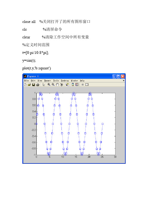
close all %关闭打开了的所有图形窗口clc %清屏命令clear %清除工作空间中所有变量%定义时间范围t=[0:pi/10:8*pi];y=sin(t);plot(t,y,'b:square')close allclcclear%定义时间范围t=[0:pi/20:9*pi];grid onhold on %允许在同一坐标系下绘制不同的图形plot(t,sin(t),'r:*')plot(t,cos(t))plot(t,-cos(t),'k')%grid on %在所画出的图形坐标中添加栅格,注意用在plot之后4-1:close allclcclear%定义时间范围t=[0:pi/20:9*pi];hold on %允许在同一坐标系下绘制不同的图形plot(t,sin(t),'r:*')plot(t,cos(t))plot(t,-cos(t),'k')grid on %在所画出的图形坐标中添加栅格,注意用在plot之后hold off %覆盖旧图,自动把栅格去掉,且若要在加入栅格就%必须把grid on加在plot后面plot(t,-sin(t))grid on%主程序exp2_10.mglobal a %声明变量a为全局变量x=1:100;a=3;c=prods(x) %调用子程序prods.m%子程序prods.m% function result=prods(x)% global a% result=a*sum(x);%声明了与主程序一样的全局变量a,以便在子程序中可以%使用主程序中定义的变量答案:15150exmdl2_1.mclearclose allclct=[0:pi/20:5*pi];figure(1)plot(t,out)grid onxlabel('time')ylabel('magnitude')exp2_1.mclc %清屏clear %从内存中清除变量和函数more onecho on%求矩阵与矩阵的乘积,矩阵与向量的乘积A=[5 6 7;9 4 6;4 3 6]B=[3 4 5;5 7 9;7 3 1]C=A*BY=A*Xmore offecho off答案:%求矩阵与矩阵的乘积,矩阵与向量的乘积A=[5 6 7;9 4 6;4 3 6]A =5 6 79 4 64 3 6B=[3 4 5;5 7 9;7 3 1]B =3 4 55 7 97 3 1X=[5 ;7;8]X =578C=A*BC =94 83 8689 82 8769 55 53Y=A*XY =12189more offecho offexp2_2.mclcclearmore onecho on%为便于理解,在程序等执行过程中显示程序的表达式a=16;b=12;c=3;d=4;e=a+b-c*df=e/2k=e\2h=c^3g=e+f+ ...2+1-9aa=sin(g)abs(aa)bb=2+3jcc=conj(bb)rbb=real(bb) log(rbb) sqrt(rbb) exp(rbb) echo off more offa=16;b=12;c=3;d=4;e=a+b-c*de =16f=e/2f =8k=e\2k =0.1250h=c^3h =27g=e+f+ ...2+1-9g =18aa=sin(g)aa =-0.7510abs(aa)ans =0.7510bb=2+3jbb =2.0000 +3.0000i cc=conj(bb)cc =2.0000 -3.0000i rbb=real(bb)rbb =2log(rbb)ans =0.6931sqrt(rbb)ans =1.4142exp(rbb)ans =7.3891echo offans =7.3891exp2_5.m%绘制单位圆clearclose allclc%定义时间范围t=[0:0.01:2*pi];x=sin(t);y=cos(t);plot(x,y)axis([-1.5 1.5 -1.5 1.5])%限定x轴和y轴的显示范围grid onaxis('equal')%axis([xmin,xmax,ymin,ymax])函数来调整图轴的范围:答案:exp2_5_.mclearclose allclct=[0:pi/20:5*pi];plot(t,sin(t),'r:*')axis([0 5*pi -1.5 1.5 ])%给x轴和y轴命名xlabel('t(deg)')ylabel('magnitude')%给图形加标题title('sine wave from zero to 5\pi')%在指定位置创建说明性文字text(pi/2,sin(pi/2),'\bullet\leftarrow The sin(t) at t=2')%图形文字标示命令的使用clearclose allclct=[0:pi/20:5*pi];plot(t,sin(t),'r:*')axis([0 5*pi -1.5 1.5 ])%给x轴和y轴命名xlabel('t(deg)')ylabel('magnitude')%给图形加标题title('sine wave from zero to 5\pi')%在指定位置创建说明性文字text(pi/2,sin(pi/2),'\bullet\leftarrow The sin(t) at t=2') %输入特定的字符%\pi%\alpha%\leftarrow%\rightarrow%\bullet(点号)hold onplot(t,cos(t))%区分图形上不同的曲线legend('sin(t)','cos(t)')%用鼠标在特定位置输入文字gtext('文字标示命令举例') hold offexp2_6.m%图形分割命令的使用clearclose allclct=[0:pi/20:5*pi];subplot(321)plot(t,sin(t))axis([0 16 -1.5 1.5]) xlabel('t(deg)') ylabel('magnitude') grid ontitle('sin(t)') subplot(322)plot(t,-sin(t))axis([0 16 -1.5 1.5]) xlabel('t(deg)') ylabel('magnitude') grid ontitle('-sin(t)') subplot(323)plot(t,cos(t))axis([0 16 -1.5 1.5]) xlabel('t(deg)') ylabel('magnitude') grid ontitle('cos(t)') subplot(324)plot(t,-cos(t))axis([0 16 -1.5 1.5]) xlabel('t(deg)') ylabel('magnitude') grid ontitle('-cos(t)') subplot(325) subplot(326)exp2_7.mclcclear%绘制对应于每个输入x的输出y的高度条形图subplot(221)x=[1 2 3 4 5 6 7 8 9 10];y=[5 6 3 4 8 1 10 3 5 6];bar(x,y)%绘制x1在以y1为中心的区间中分布的个数条形图subplot(222)x1=randn(1,1000);%生成1000个各随机数y1=-3:0.1:3;hist(x1,y1)%绘制y2对应于x2的梯形图subplot(223)x2=0:0.1:10;y2=1./(x2.^3-2.*x2+4);stairs(x2,y2)%绘制y3对应于x3的散点图subplot(224)x3=0:0.1:10;y3=1./(x2.^3-2.*x2+4);stem(x3,y3)exp2_8.mecho off % 不显示程序内容%clear allclearclca=4;b=6disp('暂停,请按任意键继续') % disp指令可以用来显示字符pause % 暂停,直到用户按任意键echo on% 显示程序内容,注意matlab默认是不显示c=a+b% 暂时把控制权交给键盘(在命令窗口中出现k提示符), % 输入return,回车后退出,继续执行下面的语句。
matlab基本语句及语法
matlab基本语句及语法一、基本语法1. 变量定义与赋值:在MATLAB中,可以使用等号(=)将一个数值或表达式赋值给一个变量。
例如:a = 5; 表示将数值5赋值给变量a。
2. 注释:在MATLAB中,可以使用百分号(%)来添加注释,以便于代码的阅读和理解。
例如:% 这是一条注释。
3. 函数的定义与调用:在MATLAB中,可以使用关键字function 来定义函数,并使用函数名进行调用。
例如:function result = add(a, b) 表示定义了一个名为add的函数,该函数接受两个参数a 和b,并返回一个结果result。
4. 条件语句:在MATLAB中,可以使用if语句来实现条件判断。
例如:if a > b 表示如果a大于b,则执行if语句块中的代码。
5. 循环语句:在MATLAB中,可以使用for循环和while循环来实现循环操作。
例如:for i = 1:10 表示从1循环到10,每次循环中i 的值递增1。
6. 矩阵的定义与操作:在MATLAB中,可以使用方括号([])来定义矩阵,并使用各种运算符进行矩阵的操作。
例如:A = [1 2; 3 4] 表示定义了一个2x2的矩阵A。
7. 字符串的操作:在MATLAB中,可以使用单引号('')来定义字符串,并使用加号(+)来进行字符串的拼接。
例如:str = 'Hello' + 'World' 表示将字符串'Hello'和'World'进行拼接。
8. 文件的读写:在MATLAB中,可以使用fopen、fread、fwrite 等函数来进行文件的读写操作。
例如:fid = fopen('file.txt', 'w') 表示打开一个名为file.txt的文件,并以写入模式打开。
9. 图形绘制:在MATLAB中,可以使用plot、scatter、histogram等函数来进行图形的绘制。
MATLAB程序运行结果

closeall %关闭打开了的所有图形窗口clc %清屏命令clear%清除工作空间中所有变量%定义时间范围t=[0:pi/10:8*pi];y=sin(t);plot(t,y,'b:square')closeallclcclear%定义时间范围t=[0:pi/20:9*pi];grid onhold on %允许在同一坐标系下绘制不同的图形plot(t,sin(t),'r:*')plot(t,cos(t))plot(t,-cos(t),'k')%grid on %在所画出的图形坐标中添加栅格,注意用在pl ot之后4-1:closeallclcclear%定义时间范围t=[0:pi/20:9*pi];hold on %允许在同一坐标系下绘制不同的图形plot(t,sin(t),'r:*')plot(t,cos(t))plot(t,-cos(t),'k')grid on %在所画出的图形坐标中添加栅格,注意用在pl ot之后hold off %覆盖旧图,自动把栅格去掉,且若要在加入栅格就%必须把gri d on加在pl ot后面plot(t,-sin(t))grid on%主程序exp2_10.mglobal a %声明变量a为全局变量x=1:100;a=3;c=prods(x) %调用子程序p rods.m%子程序pro d s.m% functi on result=prods(x)% global a% result=a*sum(x);%声明了与主程序一样的全局变量a,以便在子程序中可以%使用主程序中定义的变量答案:15150exmdl2_1.mclearcloseallclct=[0:pi/20:5*pi];figure(1)plot(t,out)grid onxlabel('time')ylabel('magnit ude')exp2_1.mclc %清屏clear%从内存中清除变量和函数more onecho on%求矩阵与矩阵的乘积,矩阵与向量的乘积A=[5 6 7;9 4 6;4 3 6]B=[3 4 5;5 7 9;7 3 1]C=A*BY=A*Xmore offecho off答案:%求矩阵与矩阵的乘积,矩阵与向量的乘积A=[5 6 7;9 4 6;4 3 6]A =5 6 79 4 64 3 6B=[3 4 5;5 7 9;7 3 1]B =3 4 55 7 97 3 1X=[5 ;7;8]X =578C=A*BC =94 83 8689 82 8769 55 53Y=A*XY =12189more offecho offexp2_2.mclcclearmore onecho on%为便于理解,在程序等执行过程中显示程序的表达式a=16;b=12;c=3;d=4;e=a+b-c*df=e/2k=e\2h=c^3g=e+f+ ...2+1-9aa=sin(g)abs(aa)bb=2+3jcc=conj(bb)rbb=real(bb) log(rbb) sqrt(rbb) exp(rbb) echo off more offa=16;b=12;c=3;d=4;e=a+b-c*de =16f=e/2f =8k=e\2k =0.1250h=c^3h =27g=e+f+ ...2+1-9g =18aa=sin(g)aa =-0.7510abs(aa)ans =0.7510bb=2+3jbb =2.0000 +3.0000icc=conj(bb)cc =2.0000 -3.0000irbb=real(bb)rbb =2log(rbb)ans =0.6931sqrt(rbb)ans =1.4142exp(rbb)ans =7.3891echo offans =7.3891exp2_5.m%绘制单位圆clearcloseallclc%定义时间范围t=[0:0.01:2*pi];x=sin(t);y=cos(t);plot(x,y)axis([-1.5 1.5 -1.5 1.5])%限定x轴和y轴的显示范围grid onaxis('equal')%axis([xmin,xmax,ymin,ymax])函数来调整图轴的范围:答案:exp2_5_.mclearcloseallclct=[0:pi/20:5*pi];plot(t,sin(t),'r:*')axis([0 5*pi -1.5 1.5 ])%给x轴和y轴命名xlabel('t(deg)')ylabel('magnit ude')%给图形加标题title('sine wave from zero to 5\pi')%在指定位置创建说明性文字text(pi/2,sin(pi/2),'\bullet\leftar row The sin(t) at t=2')%图形文字标示命令的使用clearcloseallclct=[0:pi/20:5*pi];plot(t,sin(t),'r:*')axis([0 5*pi -1.5 1.5 ])%给x轴和y轴命名xlabel('t(deg)')ylabel('magnit ude')%给图形加标题title('sine wave from zero to 5\pi')%在指定位置创建说明性文字text(pi/2,sin(pi/2),'\bullet\leftar row The sin(t) at t=2') %输入特定的字符%\pi%\alpha%\leftar row%\righta rrow%\bullet(点号)hold onplot(t,cos(t))%区分图形上不同的曲线legend('sin(t)','cos(t)')%用鼠标在特定位置输入文字gtext('文字标示命令举例') hold offexp2_6.m%图形分割命令的使用clearcloseallclct=[0:pi/20:5*pi];subplo t(321)plot(t,sin(t))axis([0 16 -1.5 1.5]) xlabel('t(deg)') ylabel('magnit ude') grid ontitle('sin(t)')subplo t(322)plot(t,-sin(t))axis([0 16 -1.5 1.5]) xlabel('t(deg)') ylabel('magnit ude') grid ontitle('-sin(t)') subplo t(323)plot(t,cos(t))axis([0 16 -1.5 1.5]) xlabel('t(deg)') ylabel('magnit ude') grid ontitle('cos(t)')subplo t(324)plot(t,-cos(t))axis([0 16 -1.5 1.5]) xlabel('t(deg)') ylabel('magnit ude') grid ontitle('-cos(t)') subplo t(325) subplo t(326)exp2_7.mclcclear%绘制对应于每个输入x的输出y的高度条形图subplo t(221)x=[1 2 3 4 5 6 7 8 9 10];y=[5 6 3 4 8 1 10 3 5 6];bar(x,y)%绘制x1在以y1为中心的区间中分布的个数条形图subplo t(222)x1=randn(1,1000);%生成1000个各随机数y1=-3:0.1:3;hist(x1,y1)%绘制y2对应于x2的梯形图subplo t(223)x2=0:0.1:10;y2=1./(x2.^3-2.*x2+4);stairs(x2,y2)%绘制y3对应于x3的散点图subplo t(224)x3=0:0.1:10;y3=1./(x2.^3-2.*x2+4);stem(x3,y3)exp2_8.mecho off % 不显示程序内容%clearallclearclca=4;b=6disp('暂停,请按任意键继续') % disp指令可以用来显示字符pause% 暂停,直到用户按任意键echo on% 显示程序内容,注意matl ab默认是不显示c=a+b% 暂时把控制权交给键盘(在命令窗口中出现k提示符), % 输入retu rn,回车后退出,继续执行下面的语句。
MATLAB程序代码

0.0444
B =
679.6289
595.7766
x =
29.9993
y =
0.1500
dxk =
37.2723
dyk =
0.1500
B =
689.1351
592.6738
x =
39.9972
y =
0.3555
dxk =
47.2702
dyk =
0.3555
B =
698.6719
589.6662
y0=604.47 %%%JD0的坐标
x1=757.119
y1=569.527 %%%JD1的坐标
dx=x0-x1
dy=y0-y1
L=(dx^2+dy^2)^0.5 %JD1到ID2的距离
T=T1(12,28,37) %%%切线长
xk0=T-L
yk0=0 %JD0的局部坐标
xk1=T
yk1=0 %JD1的局部坐标
matlab程序代码以及运行结果functiondetailedexplanationgoesherex0653779y060447jd0的坐标x1757119y1569527jd1的坐标dxx0x1dyy0y1ldx2dy205jd1到id2的距离tt1122837切线长xk0tlyk00jd2的局部坐标c09473s03203预设cos和sin求左端缓和曲线x局部坐标求左端缓和曲线y局部坐标dxkxxk0dykyyk0bx0
%求左端缓和曲线Y局部坐标
dxk=x-xk0
dyk=y-yk0
B=[x0;y0]+[c,-s;s,c]*[dxk;dyk]
%进行坐标换算
end
matlab中while 1的用法

题目:深入探讨MATLAB中while 1的用法一、引言MATLAB(Matrix Laboratory)是一种强大的数学软件,广泛应用于工程、科学领域的数据分析和可视化。
在MATLAB中,while循环是一种常见的控制结构,用于根据特定条件重复执行一段代码。
本文将深入探讨MATLAB中while 1的用法,以便读者更好地理解和应用该特性。
二、while 1的基本语法在MATLAB中,while 1是一种常见的编程技巧,用于创建一个无限循环。
它的基本语法如下:```while 1循环体代码end```其中,while关键字后的条件表达式为1,表示条件始终为真,因此循环将无限执行下去。
在循环体内部,可以编写一系列需重复执行的代码逻辑。
三、while 1的应用场景1. 任务监控在实际编程中,while 1常用于任务监控的场景。
当需要不断监听外部输入或者定时执行某个任务时,可以使用while 1构建一个持续监控的循环。
2. 实时数据处理MATLAB常用于处理实时数据,而while 1循环则可以保证对实时数据进行持续性的处理和分析。
这种用法通常用于传感器数据的采集与处理,网络数据的实时传输等场景。
3. 程序测试与调试在程序测试和调试阶段,while 1循环也具有重要作用。
它能够让程序持续执行,方便程序员观察程序行为、调试代码逻辑、捕捉异常等。
4. 无限循环有些情况下,程序需要执行一个没有终止条件的循环。
此时,while 1循环可派上用场,实现程序的无限循环。
四、while 1的注意事项1. 防止死循环使用while 1循环时,务必小心防止死循环。
在循环体内部必须有合适的跳出机制,否则程序将陷入无尽的循环之中,造成系统资源的浪费和程序的崩溃。
2. 兼顾性能和效率在使用while 1循环时,要注意兼顾性能和效率。
循环体内的代码应尽量简洁高效,避免不必要的计算和重复操作,以提高程序的执行效率。
3. 注意程序运行时间无限循环可能导致程序长时间运行,因此需特别留意程序的运行时间。
MATLAB应用实验指导书1234-结果

MATLAB应用实验指导书1234-结果************************ MATLAB语言实验指导书************************中国矿业大学信息与电气工程学院2014年3月实验一 MATLAB 工作环境熟悉及基本运算一、实验目的:熟悉MATLAB 的工作环境,学会使用MATLAB 进行一些简单的运算。
掌握基本的矩阵运算及常用的函数。
二、实验内容:MATLAB 的启动和退出,熟悉MATLAB 的桌面(Desktop ),包括菜单(Menu )、工具条(Toolbar )、命令窗口(Command Window)、历史命令窗口、工作空间(Workspace)等;完成一些基本的矩阵操作;学习使用在线帮助系统。
三、实验步骤:1、启动MATLAB ,熟悉MATLAB 的桌面。
2、在命令窗口执行命令完成以下运算,观察workspace 的变化,记录运算结果。
(1)(365-522-70) 3 = (2)area=pi*^2 = (3)已知x=3,y=4,在MATLAB 中求z :()232y x y x z -== 576 (4)将下面的矩阵赋值给变量m1,在workspace 中察看m1在内存中占用的字节数。
m1=11514412679810115133216 执行以下命令>>m1( 2 , 3 )=10 >>m1( 11 )=6>>m1( : , 3 )= 3 10 6 15>>m1( 2 : 3 , 1 : 3 )=[ 5 11 10;9 7 6]>>m1( 1 ,4 ) + m1( 2 ,3 ) + m1( 3 ,2 ) + m1( 4 ,1)=34(5)执行命令>>help abs查看函数abs 的用法及用途,计算abs( 3 + 4i )=5 (6)执行命令>>x=0::6*pi; >>y=5*sin(x); >>plot(x,y)(7)运行MATLAB 的演示程序,>>demo ,以便对MATLAB 有一个总体了解。
Matlab程序编制简介
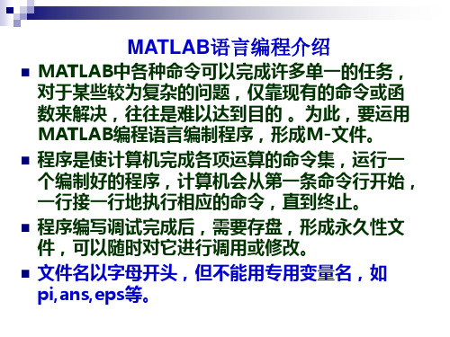
的正实根. 例1:用二分法求函数 :用二分法求函数x^2-2=0的正实根 的正实根
f ( x) = x2 2, [a, b] = [1,2], f (a) f (b) < 0
1)c = (a + b) / 2 : if f (c) = 0(| f (c) |< r), g = c;
elseif f (c) f (a) < 0 b = c, f (b) = f (c);
例2:求阶乘:p=1×2 × 3 × … × n=n! :求阶乘: ×
n=input('请输入 n= ') 请输入 p=1 for i=1:n p=p*i fprintf(' i=%.0f, p=%.0f\n ',i,p) end aa2.m
例3:求e:e=1+1+1/2!+1/3!+…+1/n! : : n=input('请输入 n= ') 请输入 p=1;e=1 for i=1:n p=p*i p1=1/p e=e+p1 fprintf(' i=%.0f, p=%.0f, e=%.8f \n ',i,p,e); end
a=input(‘a=‘) b=input(‘b=‘) n=input(‘n=‘) [p,q]=fun1(a,b,n); fprintf(‘(a+b)^n=%.4f,(a-b)^n=%.4f\n’,p,q)
数值计算问题举例
问题: 问题:求无理数的近似值 n A ( A > 1, n ≥ 2 ) 的近似值,再设计通用函数. 先求 2 的近似值,再设计通用函数.
例7:建立符号函数 :建立符号函数sgn(x)
function sn=sgn(x) if x>0 sn=1; elseif x==0 sn=0; else sn=-1; end 作为文件名存盘, 以sgn作为文件名存盘,即建立了函数。 作为文件名存盘 即建立了函数。 调用: 调用: 在命令区执行 : sn=sgn(10)或sn=sgn(-2) 或