8 基于几何光学的单幅二维图像深度估计

合集下载

基于几何光学的单幅二维图像三维重建

第六章基于几何光学的单幅二维图像三维重建单幅二维图像进行三维重建一直是计算机视觉领域的难题，因为每一图像点都有无限多个场景点与之对应。

故从光学成像的角度分析，单幅二维图像三维重建问题好像不存在较为通用的解决方案。

然而反思人类自身视觉经验，仅用一只眼睛观察单幅二维图像，同样能感觉到栩栩如生的三维世界。

而且完成这一过程是不需要任何意识努力，好像是全部自动进行的。

这些表明人类视觉系统能轻松解决这个问题。

人眼与照相机的光学成像机制几乎完全相同，故模拟人类视觉系统，计算机对单幅二维图像进行三维重建又是完全有可能的，这正是本章研究工作的基本思路与逻辑起点。

单幅二维图像三维重建问题的难点在于对单幅二维图像深度估计，本文第五章提出解决解决这一问题的有效方法。

本章将在第五章提出的深度模型(图5-1)的基础上，研究基于几何光学的二维图像三维重建算法。

本质上讲，大小恒常性变换就是一种单幅二维图像三维重建过程。

故本章也对基于心理学的重建方法与基于几何光学的重建方法进行比较，继续探讨在计算机视觉中应用视觉心理学结论的适应性问题。

6.1引言计算机视觉的研究目标是使计算机具有通过二维图像认知三维环境信息的能力，然后达到认识世界的目的，故二维图像三维重建一直是计算机视觉的主要内容。

计算机视觉奠基人Marr名著《Vision》的中心内容就是力图阐述如何从二维图像出发，重建客观世界物体的三维模型。

从上世纪60年代以来，许多学者从不同的角度，提出了不同的三维重建方法，主要分为以下五类：多相机立体视觉、光度学立体视觉、用阴影求形状、基于模型重建及三灭点重建等，下面分别叙述。

(1)多相机立体视觉[Stewenius 2005][Rajagopalan 2004][Cheng 2005] [Williams 2005] [马颂德1998, pp72-93]。

这是指用两架或多架照相机对同一空间场景进行拍照，得到同一场景不同视角的两幅或多幅图像，并用这些图像恢复三维空间几何形状的方法。

基于监督学习的单幅图像深度估计综述

基于监督学习的单幅图像深度估计综述
毕天腾;刘越;翁冬冬;王涌天
【期刊名称】《计算机辅助设计与图形学学报》
【年(卷),期】2018(030)008
【摘要】单幅图像深度估计是三维重建中基于图像获取场景深度的重要技术,也是计算机视觉中的经典问题,近年来,基于监督学习的单幅图像深度估计发展迅速.文中介绍了基于监督学习的单幅图像深度估计及其模型和优化方法;分析了现有的参数学习、非参数学习、深度学习3类方法及每类方法的国内外研究现状及优缺点;最后对基于监督学习的单幅图像深度估计进行总结,得出了深度学习框架下的单幅图像深度估计是未来研究的发展趋势和重点.
【总页数】11页(P1383-1393)
【作者】毕天腾;刘越;翁冬冬;王涌天
【作者单位】北京理工大学光电学院北京 100081;北京理工大学光电学院北京100081;北京理工大学光电学院北京 100081;北京理工大学光电学院北京100081
【正文语种】中文
【中图分类】TP391.41
【相关文献】
1.基于多尺度纹理能量测度的单幅图像深度估计 [J], 蓝建梁;丁友东;黄东晋;吴冏
2.基于非参数化采样的单幅图像深度估计 [J], 朱尧;喻秋
3.基于单幅图像的深度非连续性估计 [J], 马祥音; 查红彬
4.基于自监督学习的番茄植株图像深度估计方法 [J], 周云成; 许童羽; 邓寒冰; 苗腾; 吴琼
5.基于多通道卷积神经网络的单幅图像深度估计 [J], 朱丙丽; 高晓琴; 阮玲英
因版权原因，仅展示原文概要，查看原文内容请购买。

单目深度估计的基础

单目深度估计的基础单目深度估计是利用单个摄像头或图像来推测场景中物体的深度信息的技术。

它是计算机视觉和机器视觉领域的一个重要任务，具有广泛的应用，如增强现实、自动驾驶、机器人导航等。

单目深度估计的基础是基于图像中的视觉几何关系来推断深度。

以下是几种常见的基于单目图像的深度估计方法：1.视差法（Disparity-basedmethods）：这种方法使用了立体视觉的原理。

通过计算左右视图之间的视差（即对应像素的水平偏移），可以估计出物体的深度信息。

这种方法需要至少两个摄像头或多个图像，例如双目摄像头或多目摄像头系统。

2.结构光法（Structured-lightmethods）：这种方法使用投射结构光的方式，通过分析光斑在场景中的形变情况来推测深度。

常见的结构光方法包括使用投影仪投射特殊的光纹或条纹，并通过摄像头观察光纹的形变来计算深度。

3.光流法（Opticalflowmethods）：这种方法基于物体在图像序列中的运动信息来推断深度。

通过分析图像中的像素运动模式，可以计算出物体的相对深度。

光流方法需要至少两个连续帧的图像序列。

4.基于学习的方法（Learning-basedmethods）：近年来，深度学习技术的发展为单目深度估计带来了显著的进展。

通过使用大量带有深度标注的数据进行训练，可以构建深度估计模型。

这些模型可以通过输入单目图像直接输出对应的深度图或深度估计结果。

这些方法各有优劣，可以根据具体的应用场景和需求选择适合的方法。

此外，单目深度估计也可以与其他传感器（如惯性测量单元、激光雷达等）的数据进行融合，以提高深度估计的准确性和稳定性。

1/ 1。

Depth Estimation_CVPR2015

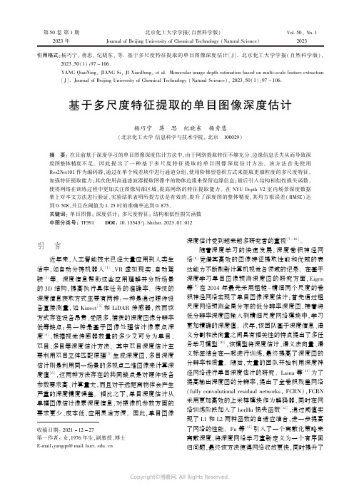
Deep Convolutional Neural Fields for Depth Estimation from a Single Image ∗Fayao Liu 1,Chunhua Shen 1,2,Guosheng Lin 1,21The University of Adelaide,Australia 2Australian Centre for Robotic VisionAbstractWe consider the problem of depth estimation from a sin-gle monocular image in this work.It is a challenging task as no reliable depth cues are available,e.g .,stereo corre-spondences,motions etc .Previous efforts have been focus-ing on exploiting geometric priors or additional sources of information,with all using hand-crafted features.Recently,there is mounting evidence that features from deep convo-lutional neural networks (CNN)are setting new records for various vision applications.On the other hand,considering the continuous characteristic of the depth values,depth esti-mations can be naturally formulated into a continuous con-ditional random ﬁeld (CRF)learning problem.Therefore,we in this paper present a deep convolutional neural ﬁeld model for estimating depths from a single image,aiming to jointly explore the capacity of deep CNN and continuous CRF.Speciﬁcally,we propose a deep structured learning scheme which learns the unary and pairwise potentials of continuous CRF in a uniﬁed deep CNN framework.The proposed method can be used for depth estimations of general scenes with no geometric priors nor any extra in-formation injected.In our case,the integral of the partition function can be analytically calculated,thus we can exactly solve the log-likelihood optimization.Moreover,solving the MAP problem for predicting depths of a new image is highly efﬁcient as closed-form solutions exist.We experimentally demonstrate that the proposed method outperforms state-of-the-art depth estimation methods on both indoor and out-door scene datasets.1.IntroductionEstimating depths from a single monocular image de-picting general scenes is a fundamental problem in com-puter vision,which has found wide applications in scene un-derstanding,3D modelling,robotics,etc .It is a notoriously ill-posed problem,as one captured image may correspond∗Thiswork is in part supported by ARC Grants FT120100969,LP120200485,LP130100156.Correspondence should be addressed to C.Shen (email:chhshen@).to numerous real world scenes [1].Whereas for humans,inferring the underlying 3D structure from a single image is of little difﬁculties,it remains a challenging task for com-puter vision algorithms as no reliable cues can be exploited,such as temporal information,stereo correspondences,etc .Previous works mainly focus on enforcing geometric as-sumptions,e.g .,box models,to infer the spatial layout of a room [2,3]or outdoor scenes [4].These models come with innate restrictions,which are limitations to model only particular scene structures and therefore not applicable for general scene depth ter on,non-parametric methods [5]are explored,which consists of candidate im-ages retrieval,scene alignment and then depth infer using optimizations with smoothness constraints.This is based on the assumption that scenes with semantic similar appear-ances should have similar depth distributions when densely aligned.However,this method is prone to propagate errors through the different decoupled stages and relies heavily on building a reasonable sized image database to perform the candidates retrieval.In recent years,efforts have been made towards incorporating additional sources of informa-tion,e.g .,user annotations [6],semantic labellings [7,8].In the recent work of [8],Ladicky et al .have shown that jointly performing depth estimation and semantic labelling can beneﬁt each other.However,they do need to hand-annotate the semantic labels of the images beforehand as such ground-truth information are generally not available.Nevertheless,all these methods use hand-crafted features.Different from the previous efforts,we propose to formu-late the depth estimation as a deep continuous CRF learning problem,without relying on any geometric priors nor any extra information.Conditional Random Fields (CRF)[9]are popular graphical models used for structured predic-tion.While extensively studied in classiﬁcation (discrete)domains,CRF has been less explored for regression (con-tinuous)problems.One of the pioneer work on continuous CRF can be attributed to [10],in which it was proposed for global ranking in document retrieval.Under certain con-straints,they can directly solve the maximum likelihood optimization as the partition function can be analytically calculated.Since then,continuous CRF has been applied a r X i v :1411.6387v 2 [c s .C V ] 18 D e c 2014for solving various structured regression problems,e.g.,re-mote sensing[11,12],image denoising[12].Motivated by all these successes,we here propose to use it for depth esti-mation,given the continuous nature of the depth values,and learn the potential functions in a deep convolutional neural network(CNN).Recent years have witnessed the prosperity of the deep convolutional neural network(CNN).CNN features have been setting new records for a wide variety of vision appli-cations[13].Despite all the successes in classiﬁcation prob-lems,deep CNN has been less explored for structured learn-ing problems,i.e.,joint training of a deep CNN and a graph-ical model,which is a relatively new and not well addressed problem.To our knowledge,no such model has been suc-cessfully used for depth estimations.We here bridge this gap by jointly exploring CNN and continuous CRF.To sum up,we highlight the main contributions of this work as follows:•We propose a deep convolutional neuralﬁeld model for depth estimations by exploring CNN and continuous CRF.Given the continuous nature of the depth values, the partition function in the probability density func-tion can be analytically calculated,therefore we can directly solve the log-likelihood optimization without any approximations.The gradients can be exactly cal-culated in the back propagation training.Moreover, solving the MAP problem for predicting the depth ofa new image is highly efﬁcient since closed form solu-tions exist.•We jointly learn the unary and pairwise potentials of the CRF in a uniﬁed deep CNN framework,which is trained using back propagation.•We demonstrate that the proposed method outperforms state-of-the-art results of depth estimation on both in-door and outdoor scene datasets.2.Related workPrior works[7,14,15]typically formulate the depth es-timation as a Markov Random Field(MRF)learning prob-lem.As exact MRF learning and inference are intractable in general,most of these approaches employ approximation methods,e.g.,multi-conditional learning(MCL),particle belief propagation(PBP).Predicting the depths of a new image is inefﬁcient,taking around4-5s in[15]and even longer(30s)in[7].To make things worse,these methods suffer from lacking ofﬂexibility in that[14,15]rely on hor-izontal alignment of images and[7]requires the semantic labellings of the training data available beforehand.More recently,Liu et al.[16]propose a discrete-continuous CRF model to take into consideration the relations between adja-cent superpixels,e.g.,occlusions.They also need to use approximation methods for learning and MAP inference.Besides,their method relies on image retrievals to obtain a reasonable initialization.By contrast,we here present a deep continuous CRF model in which we can directly solve the log-likelihood optimization without any approximations as the partition function can be analytically calculated.Pre-dicting the depth of a new image is highly efﬁcient since closed form solution exists.Moreover,our model do not inject any geometric priors nor any extra information.On the other hand,previous methods[5,7,8,15,16]all use hand-crafted features in their work,e.g.,texton,GIST, SIFT,PHOG,object bank,etc.In contrast,we learn deep CNN for constructing unary and pairwise potentials of CRF. By jointly exploring the capacity of CNN and continuous CRF,our method outperforms state-of-the-art methods on both indoor and outdoor scene depth estimations.Perhaps the most related work is the recent work of[1],which is concurrent to our work here.They train two CNNs for depth map prediction from a single image.However,our method bears substantial differences from theirs.They use the CNN as a black-box by directly regressing the depth map from an input image through convolutions.In contrast, we use CRF to explicitly model the relations of neighbour-ing superpixels,and learn the potentials in a uniﬁed CNN framework.One potential drawback of the method in[1]is that it tends to learn depths with location preferences,which is prone toﬁt into speciﬁc layouts.This partly explains why they have to collect a large number of labelled data to cover all possible layouts for training the networks(they collect extra training images using depth sensors),which is in the millions as reported in[1].Instead,our method en-joys translation invariance as we do not encode superpixel coordinates into the unary potentials,and can train on stan-dard dataset to get competetive performance without using additional training data.Furthermore,the predicted depth map of[1]is1/4-resolution of the original input image with some border areas lost,while our method does not have this limitation.In the most recent work of[17],Tompson et al.present a hybrid architecture for jointly training a deep CNN and an MRF for human pose estimation.Theyﬁrst train a unary term and a spatial model separately,then jointly learn them as aﬁne tuning step.Duringﬁne tuning of the whole model, they simply remove the partition function in the likelihood to have a loose approximation.In contrast,our model performs continuous variables prediction.We can directly solve the log-likelihood optimization without using approx-imations as the partition function is integrable and can be analytically calculated.Moreover,during prediction,we have closed-form solution for the MAP inference.3.Deep convolutional neuralﬁeldsWe present the details of our deep convolutional neural ﬁeld model for depth estimation in this section.Unless oth-CRF loss layerparameters parameters (pairwise)Neighbouring superpixel Negative log-likelihood:Supperpixel whereFigure 1:An illustration of our deep convolutional neural ﬁeld model for depth estimation.The input image is ﬁrst over-segmented into superpixels.In the unary part,for a superpixel p ,we crop the image patch centred around its centroid,then resize and feed it to a CNN which is composed of 5convolutional and 4fully-connected layers (details refer to Fig.2).In the pairwise part,for a pair of neighbouring superpixels (p,q ),we consider K types of similarities,and feed them into a fully-connected layer.The outputs of unary part and the pairwise part are then fed to the CRF structured loss layer,which minimizes the negative log-likelihood.Predicting the depths of a new image x is to maximize the conditional probability Pr(y |x ),which has closed-form solutions (see Sec.3.3for details).erwise stated,we use boldfaced uppercase and lowercase letters to denote matrices and column vectors respectively.3.1.OverviewThe goal here is to infer the depth of each pixel in a single image depicting general scenes.Following the work of [7,15,16],we make the common assumption that an im-age is composed of small homogeneous regions (superpix-els)and consider the graphical model composed of nodes deﬁned on superpixels.Kindly note that our framework is ﬂexible that can work on pixels or superpixels.Each su-perpixel is portrayed by the depth of its centroid.Let x be an image and y =[y 1,...,y n ] ∈R n be a vector of con-tinuous depth values corresponding to all n superpixels in x .Similar to conventional CRF,we model the conditional probability distribution of the data with the following den-sity function:Pr(y |x )=1Z(x )exp(−E (y ,x )),(1)where E is the energy function;Z is the partition functiondeﬁned as:Z(x )=yexp {−E (y ,x )}d y .(2)Here,because y is continuous,the integral in Eq.(A.1)can be analytically calculated under certain circumstances,which we will show in Sec.3.3.This is different from the discrete case,in which approximation methods need to be applied.To predict the depths of a new image,we solve the maximum a posteriori (MAP)inference problem:y =argmax yPr(y |x ).(3)We formulate the energy function as a typical combina-tion of unary potentials U and pairwise potentials V over the nodes (superpixels)N and edges S of the image x :E (y ,x )= p ∈NU (y p ,x )+(p,q )∈SV (y p ,y q ,x ).(4)The unary term U aims to regress the depth value from asingle superpixel.The pairwise term V encourages neigh-bouring superpixels with similar appearances to take similar depths.We aim to jointly learn U and V in a uniﬁed CNN framework.In Fig.1,we show a sketch of our deep convolutional neural ﬁeld model for depth estimation.As we can see,the whole network is composed of a unary part,a pairwise part and a CRF loss layer.For an input image,which has224224Figure 2:Detailed network architecture of the unary part in Fig.1.been over-segmented into n superpixels,we consider image patches centred around each superpxiel centroid.The unary part then takes all the image patches as input and feed each of them to a CNN and output an n -dimentional vector con-taining regressed depth values of the n superpixels.The network for the unary part is composed of 5convolutional and 4fully-connected layers with details in Fig.2.Kindly note that the CNN parameters are shared across all the su-perpixels.The pairwise part takes similarity vectors (each with K components)of all neighbouring superpixel pairs as input and feed each of them to a fully-connected layer (parameters are shared among different pairs),then output a vector containing all the 1-dimentional similarities for each of the neighbouring superpixel pair.The CRF loss layer takes as input the outputs from the unary and the pairwise parts to minimize the negative pared to the direct regression method in [1],our model possesses two potential advantages:1)We achieve translation invari-ance as we construct unary potentials irrespective of the su-perpixel’s coordinate (shown in Sec. 3.2);2)We explic-itly model the relations of neighbouring superpixels through pairwise potentials.In the following,we describe the details of potential functions involved in the energy function in Eq.(4).3.2.Potential functionsUnary potential The unary potential is constructed fromthe output of a CNN by considering the least square loss:U (y p ,x ;θ)=(y p −z p (θ))2,∀p =1,...,n.(5)Here z p is the regressed depth of the superpixel p parametrized by the CNN parameters θ.The network architecture for the unary part is depicted in Fig.2.Our CNN model in Fig.2is mainly based upon the well-known network architecture of Krizhevsky et al .[18]with modiﬁcations.It is composed of 5convolutional layers and 4fully connected layers.The input image is ﬁrst over-segmented into superpixels,then for each superpixel,we consider the image patch centred around its centroid.Each of the image patches is resized to 224×224pixels and then fed to the convolutional neural network.Note that the con-volutional and the fully-connected layers are shared across all the image patches of different superpixels.Rectiﬁed lin-ear units (ReLU)are used as activiation functions for theﬁve convolutional layers and the ﬁrst two fully connected layers.For the third fully-connected layer,we use the logis-tic function (f (x )=(1+e −x )−1)as activiation function.The last fully-connected layer plays the role of model en-semble with no activiation function followed.The output is an 1-dimentional real-valued depth for a single superpixel.Pairwise potential We construct the pairwise potential from K types of similarity observations,each of which en-forces smoothness by exploiting consistency information of neighbouring superpixels:V (y p ,y q ,x ;β)=12R pq (y p −y q )2,∀p,q =1,...,n.(6)Here R pq is the output of the network in the pairwise part (see Fig.1)from a neighbouring superpixel pair (p,q ).We use a fully-connected layer here:R pq =β[S (1)pq ,...,S (K )pq ]=K k =1βk S (k )pq ,(7)where S (k )is the k -th similarity matrix whose elements are S (k )pq (S (k )is symmetric);β=[β1,...,βk ] are the net-work parameters.From Eq.(A.4),we can see that we don’t use any activiation function.However,as our framework is general,more complicated networks can be seamlessly in-corporated for the pairwise part.In Sec .3.3,we will show that we can derive a general form for calculating the gradi-ents with respect to β(see Eq.(A.14)).To guarantee Z (x )(Eq.(A.3))is integrable,we require βk ≥0[10].We consider 3types of pairwise similarities,mea-sured by the color difference,color histogram difference and texture disparity in terms of local binary patterns(LBP)[19],which take the conventional form:S (k )pq =e −γ s (k )p −s (k )q ,k =1,2,3,where s (k )p ,s (k )q are the obser-vation values of the superpixel p ,q calculated from color,color histogram and LBP; · denotes the 2norm of a vec-tor and γis a constant.3.3.LearningWith the unary and the pairwise pontentials deﬁned in Eq.(5),(6),we can now write the energy function as:E (y ,x )= p ∈N(y p −z p )2+(p,q )∈S12R pq (y p −y q )2.(8)For ease of expression,we introduce the following notation:A =I +D −R ,(9)where I is the n ×n identity matrix;R is the matrix com-posed of R pq ;D is a diagonal matrix with D pp = q R pq .Expanding Eq.(A.2),we have:E (y ,x )=y Ay −2z y +z z .(10)Due to the quadratic terms of y in the energy function in Eq.(A.5)and the positive deﬁniteness of A ,we can analytically calculate the integral in the partition function (Eq.(A.3))as:Z (x )=yexp {−E (y ,x )}d y=(π)n 2|A |12exp {z A −1z −z z }.(11)From Eq.(A.1),(A.5),(11),we can now write the probabil-ity distribution function as (see supplementary for details):Pr(y |x )=|A |12πn 2exp −y Ay +2z y −z A −1z ,(12)where z =[z 1,...,z n ];|A |denotes the determinant of the matrix A ,and A −1the inverse of A .Then the negative log-likelihood can be written as:−log Pr(y |x )=y Ay −2z y +z A −1z(13)−12log(|A |)+n 2log(π).During learning,we minimizes the negative conditional log-likelihood of the training data.Adding regularization to θ,β,we then arrive at the ﬁnal optimization:min θ,β≥0−N i =1log Pr(y (i )|x (i );θ,β)(14)+λ12 θ 22+λ22β 22,where x (i ),y (i )denote the i -th training image and the cor-responding depth map;N is the number of training images;λ1and λ2are weight decay parameters.We use stochastic gradient descent (SGD)based back propagation to solve the optimization problem in Eq.(A.10)for learning all param-eters of the whole network.We project the solutions to the feasible set when the bounded constraints βk ≥0is vio-lated.In the following,we calculate the partial derivatives of −log Pr(y |x )with respect to the network parameters θl (one element of θ)and βk (one element of β)by using thechain rule (refer to supplementary for details):∂{−log Pr(y |x )}l =2(A −1z −y ) ∂z l,(15)∂{−log Pr(y |x )}∂βk=y Jy −z A −1JA −1z−12Tr A −1J ,(16)where Tr(·)denotes the trace of a matrix;J is an n ×n matrix with elements:J pq =−∂R pq∂βk +δ(p =q ) q ∂R pq ∂βk ,(17)where δ(·)is the indicator function,which equals 1if p =qis true and 0otherwise.From Eq.(A.13),we can see that our framework is general and more complicated networks for the pairwise part can be seamlessly incorporated.Here,in our case,with the deﬁnition of R pq in Eq.(A.4),we have∂R pq∂βk=S (k )pq .Depth prediction Predicting the depths of a new image is to solve the MAP inference in Eq.(3),in which closed form solutions exist here (details refer to supplementary):y =argmax y Pr(y |x )(18)=argmax y−y Ay +2z y =A −1z .If we discard the pairwise terms,namely R pq =0,thenEq.(18)degenerates to y =z ,which is a conventional regression model (we will report the results of this method as a baseline in the experiment).3.4.Implementation detailsWe implement the network training based on the efﬁcientCNN toolbox:VLFeat MatConvNet 1[20].Training is done on a standard desktop with an NVIDIA GTX 780GPU with 6GB memory.During each SGD iteration,around ∼700superpixel image patches need to be processed.The 6GB GPU may not be able to process all the image patches at one time.We therefore partition the superpixel image patches of one image into two parts and process them successively.Processing one image takes around 10s (including forward and backward)with ∼700superpixels when training the whole network.During implementation,we initialize the ﬁrst 6layers of the unary part in Fig.2using a CNN model trained on the ImageNet from [21].First,we do not back propa-gate through the previous 6layers by keeping them ﬁxed1VLFeatMatConvNet:/matconvnet/MethodErrorAccuracy (lower is better)(higher is better)rel log10rms δ<1.25δ<1.252δ<1.253SVR0.3130.128 1.0680.4900.7870.921SVR (smooth)0.2900.1160.9930.5140.8210.943Ours (unary only)0.2950.1170.9850.5160.8150.938Ours (pre-train)0.2570.1010.8430.5880.8680.961Ours (ﬁne-tune)0.2300.0950.8240.6140.8830.971Table 2:Baseline comparisons on the NYU v2dataset.Our method with the whole network training performs the best.MethodError (C1)Error (C2)(lower is better)(lower is better)rel log10rms rel log10rms SVR0.4330.1588.930.4290.17015.29SVR (smooth)0.3800.1408.120.3840.15515.10Ours (unary only)0.3660.1378.630.3630.14814.41Ours (pre-train)0.3310.1278.820.3240.13413.29Ours (ﬁne-tune)0.3140.1198.600.3070.12512.89Table 3:Baseline comparisons on the Make3D dataset.Our method with the whole network training performs the best.and train the rest of the network (we refer this process as pre-train)with the following settings:momentum is set to 0.9,and weight decay parameters λ1,λ2are set to 0.0005.During pre-train,the learning rate is initialized at 0.0001,and decreased by 40%every 20epoches.We then run 60epoches to report the results of pre-train (with learning rate decreased twice).The pre-train is rather efﬁcient,taking around 1hour to train on the Make3D dataset,and infer-ring the depths of a new image takes less than 0.1s.Then we train the whole network with the same momentum and weight decay.We apply dropout with ratio 0.5in the ﬁrst two fully-connected layers of Fig. 2.Training the whole network takes around 16.5hours on the Make3D dataset,and around 33hours on the NYU v2dataset.Predicting the depth of a new image from scratch takes ∼1.1s.4.ExperimentsWe evaluate on two popular datasets which are available online:the NYU v2Kinect dataset [22]and the Make3D range image dataset [15].Several measures commonly used in prior works are applied here for quantitative evaluations:•average relative error (rel):1T p |d gt p −d p |d gt p;•root mean squared error (rms): 1Tp (d gt p −d p )2;•average log 10error (log10):1T p |log 10d gtp −log 10d p |;•accuracy with threshold thr :percentage (%)ofd p s .t .:max(d gt p d p ,d pd gt p)=δ<thr ;where d gt p and d p are the ground-truth and predicted depthsrespectively at pixel indexed by p ,and T is the total number of pixels in all the evaluated images.We use SLIC [23]to segment the images into a set of non-overlapping superpixels.For each superpixel,we con-sider the image within a rectangular box centred on the cen-troid of the superpixel,which contains a large portion of its background surroundings.More speciﬁcally,we use a box size of 168×168pixels for the NYU v2and 120×120pixels for the Make3D dataset.Following [1,7,15],we transform the depths into log-scale before training.As for baseline comparisons,we consider the following settings:•SVR:We train a support vector regressor using the CNN representations from the ﬁrst 6layers of Fig.2;•SVR (smooth):We add a smoothness term to the trained SVR during prediction by solving the infer-ence problem in Eq.(18).As tuning multiple pairwise parameters is not straightforward,we only use color difference as the pairwise potential and choose the pa-rameter βby hand-tuning on a validation set;•Unary only:We replace the CRF loss layer in Fig.1with a least-square regression layer (by setting the pair-wise outputs R pq =0,p,q =1,...,n ),which degener-ates to a deep regression model trained by SGD.4.1.NYU v2:Indoor scene reconstructionThe NYU v2dataset consists of 1449RGBD images of indoor scenes,among which 795are used for training and 654for test (we use the standard training/test split provided with the dataset).Following [16],we resize the images to 427×561pixels before training.For a detailed analysis of our model,we ﬁrst compare with the three baseline methods and report the results in Ta-ble 2.From the table,several conclusions can be made:1)When trained with only unary term,deeper network is beneﬁcial for better performance,which is demonstrated by the fact that our unary only model outperforms the SVR model;2)Adding smoothness term to the SVR or our unary only model helps improve the prediction accuracy;3)Our method achieves the best performance by jointly learning the unary and the pairwise parameters in a uniﬁed deep CNN framework.Moreover,ﬁne-tuning the whole network yields further performance gain.These well demonstrate the efﬁcacy of our model.In Table 1,we compare our model with several pop-ular state-of-the-art methods.As can be observed,our method outperforms classic methods like Make3d [15],DepthTransfer [5]with large margins.Most notably,our results are signiﬁcantly better than that of [8],which jointly exploits depth estimation and semantic par-ing to the recent work of Eigen et al .[1],our method gener-ally performs on par.Our method obtains signiﬁcantly bet-ter result in terms of root mean square (rms)error.Kindly note that,to overcome overﬁt,they [1]have to collect mil-lions of additional labelled images to train their model.OneT e s t i m a geG r o u n d -t r u th E i g e n e t a l .[1]O u r s (ﬁn e -t u n e )Figure 3:Examples of qualitative comparisons on the NYUD2dataset (Best viewed on screen).Our method yields visually better predictions with sharper transitions,aligning to local details.MethodErrorAccuracy (lower is better)(higher is better)rel log10rms δ<1.25δ<1.252δ<1.253Make3d [15]0.349- 1.2140.4470.7450.897DepthTransfer [5]0.350.131 1.2---Discrete-continuous CRF [16]0.3350.127 1.06---Ladicky et al .[8]---0.5420.8290.941Eigen et al .[1]0.215-0.9070.6110.8870.971Ours (pre-train)0.2570.1010.8430.5880.8680.961Ours (ﬁne-tune)0.2300.0950.8240.6140.8830.971Table 1:Result comparisons on the NYU v2dataset.Our method performs the best in most cases.Kindly note that the results of Eigen et al .[1]are obtained by using extra training data (in the millions in total)while ours are obtained using the standard training set.possible reason is that their method captures the absolute pixel location information and they probably need a very large training set to cover all possible pixel layouts.In con-trast,we only use the standard training sets (795)without any extra data,yet we achieve comparable or even better performance.Fig.3illustrates some qualitative evalua-tions of our method compared against Eigen et al .[1](We download the predictions of [1]from the authors’website.).Compared to the predictions of [1],our method yields more visually pleasant predictions with sharper transitions,align-ing to local details.4.2.Make3D:Outdoor scene reconstructionThe Make3D dataset contains 534images depicting out-door scenes.As pointed out in [15,16],this dataset is with limitations:the maximum value of depths is 81m with far-away objects are all mapped to the one distance of 81me-ters.As a remedy,two criteria are used in [16]to report theprediction errors:(C 1)Errors are calculated only in the re-gions with the ground-truth depth less than 70meters;(C 2)Errors are calculated over the entire image.We follow this protocol to report the evaluation results.Likewise,we ﬁrst present the baseline comparisons in Table 3,from which similar conclusions can be drawn as in the NYU v2dataset.We then show the detailed results compared with several state-of-the-art methods in Table 4.As can be observed,our model with the whole network training ranks the ﬁrst in overall performance,outperform-ing the compared methods by large margins.Kindly note that the C2errors of [16]are reported with an ad-hoc post-processing step,which trains a classiﬁer to label sky pixels and set the corresponding regions to the maximum depth.In contrast,we do not employ any of those heuristics to re-ﬁne our results,yet we achieve better results in terms of relative error.Some examples of qualitative evaluations are shown in Fig.4.It is shown that our unary only model gives。

单目图像深度估计方法[发明专利]

专利名称：单目图像深度估计方法专利类型：发明专利
发明人：霍智勇,乔璐
申请号：CN202011084248.2申请日：20201012
公开号：CN112288788A
公开日：
20210129
专利内容由知识产权出版社提供
摘要：一种单目图像深度估计方法，所述方法包括：获取训练图像；将所获取的训练图像输入预先构建的深度预测网络中进行训练，得到对应的预测深度图；将所得到的预测深度图与对应的GT深度图采用排序损失、多尺度结构相似损失和多尺度尺度不变梯度匹配损失的联合损失函数进行联合损失计算，得到对应的单目深度估计图。

上述的方案，可以提高单目图像深度估计的准确性。

申请人：南京邮电大学
地址：210003 江苏省南京市鼓楼区新模范马路66号
国籍：CN
代理机构：南京苏科专利代理有限责任公司
代理人：姚姣阳
更多信息请下载全文后查看。

基于多尺度特征提取的单目图像深度估计

第50卷第1期2023年北京化工大学学报(自然科学版)Journal of Beijing University of Chemical Technology (Natural Science)Vol.50,No.12023引用格式:杨巧宁,蒋思,纪晓东,等.基于多尺度特征提取的单目图像深度估计[J].北京化工大学学报(自然科学版),2023,50(1):97-106.YANG QiaoNing,JIANG Si,JI XiaoDong,et al.Monocular image depth estimation based on multi⁃scale feature extraction [J].Journal of Beijing University of Chemical Technology (Natural Science),2023,50(1):97-106.基于多尺度特征提取的单目图像深度估计杨巧宁　蒋　思　纪晓东　杨秀慧(北京化工大学信息科学与技术学院,北京　100029)摘　要:在目前基于深度学习的单目图像深度估计方法中,由于网络提取特征不够充分㊁边缘信息丢失从而导致深度图整体精度不足㊂因此提出了一种基于多尺度特征提取的单目图像深度估计方法㊂该方法首先使用Res2Net101作为编码器,通过在单个残差块中进行通道分组,使用阶梯型卷积方式来提取更细粒度的多尺度特征,加强特征提取能力;其次使用高通滤波器提取图像中的物体边缘来保留边缘信息;最后引入结构相似性损失函数,使得网络在训练过程中更加关注图像局部区域,提高网络的特征提取能力㊂在NYU Depth V2室内场景深度数据集上对本文方法进行验证,实验结果表明所提方法是有效的,提升了深度图的整体精度,其均方根误差(RMSE)达到0.508,并且在阈值为1.25时的准确率达到0.875㊂关键词:单目图像;深度估计;多尺度特征;结构相似性损失函数中图分类号:TP391 DOI :10.13543/j.bhxbzr.2023.01.012收稿日期:20211227第一作者:女,1976年生,副教授,博士E⁃mail:yangqn@引　言近年来,人工智能技术已经大量应用到人类生活中,如自动分拣机器人[1]㊁VR 虚拟现实㊁自动驾驶[2]等㊂深度信息帮助这些应用理解并分析场景的3D 结构,提高执行具体任务的准确率㊂传统的深度信息获取方式主要有两种:一种是通过硬件设备直接测量,如Kinect [3]和LiDAR 传感器,然而该方式存在设备昂贵㊁受限多㊁捕获的深度图像分辨率低等缺点;另一种是基于图像处理估计像素点深度[4],根据视觉传感器数量的多少又可分为单目㊁双目㊁多目等深度估计方法㊂其中双目深度估计主要利用双目立体匹配原理[5]生成深度图,多目深度估计则是利用同一场景的多视点二维图像来计算深度值[6],这两种方法存在的共同缺点是对硬件设备参数要求高㊁计算量大,而且对于远距离物体会产生严重的深度精度误差㊂相比之下,单目深度估计从单幅图像估计像素深度信息,对摄像机参数方面的要求更少㊁成本低㊁应用灵活方便㊂因此,单目图像深度估计受到越来越多研究者的重视[7-16]㊂随着深度学习的快速发展,深度卷积神经网络[8]凭借其高效的图像特征提取性能和优越的表达能力不断刷新计算机视觉各领域的记录㊂在基于深度学习单目图像预测深度图的研究方面,Eigen 等[9]在2014年最先采用粗糙-精细两个尺度的卷积神经网络实现了单目图像深度估计:首先通过粗尺度网络预测全局分布的低分辨率深度图,接着将低分辨率深度图输入到精细尺度网络模块中,学习更加精确的深度值㊂次年,该团队基于深度信息㊁语义分割和法向量之间具有相关性的特点提出了多任务学习模型[10],该模型将深度估计㊁语义法向量㊁语义标签结合在一起进行训练,最终提高了深度图的分辨率和质量㊂随后,大量的团队开始利用深度神经网络进行单目深度估计的研究㊂Laina 等[11]为了提高输出深度图的分辨率,提出了全卷积残差网络(fully convolutional residual networks,FCRN),FCRN 采用更加高效的上采样模块作为解码器,同时在网络训练阶段加入了berHu 损失函数[12],通过阈值实现了L1和L2两种函数的自适应结合,进一步提高了网络的性能㊂Fu 等[13]引入了一个离散化策略来离散深度,将深度网络学习重新定义为一个有序回归问题,最终该方法使得网络收敛更快,同时提升了深度图的整体精度㊂Cao等[14]将深度估计回归任务看作一个像素级分类问题,有效避免了预测的深度值出现较大偏差的现象,获得了更准确的深度值㊂Lee等[15]提出了从绝对深度转变为相对深度的预测像素点的算法㊂Hu等[16]设计了一个新的网络架构,该架构包含编码模块㊁解码模块㊁特征融合模块㊁精细化模块4个模块,针对边缘设计了梯度损失函数,进一步提升了神经网络的训练效果㊂虽然深度学习在单目图像深度估计任务中取得了较大的进展,但是依然存在以下问题:在单目图像深度估计任务中,现实场景具有复杂性,比如物体尺寸大小不一㊁较小的物体需要背景才能被更好地识别等,这增加了网络特征提取的难度㊂现有的单目图像深度估计方法通常通过增加网络层数来提高网络提取特征能力[17-24],在这个过程中,层级之间采用固定尺度的卷积核或卷积模块对特征图提取特征,导致层级之间提取的特征尺度单一,多尺度特征提取不够充分,最终获得的深度图整体精度不高㊂针对以上问题,本文提出了一种基于多尺度特征提取的单目图像深度估计方法,该方法引入Res2Net网络作为特征提取器,以提高网络的多尺度特征提取和表达能力;其次设计了边缘增强模块,解决了网络训练过程中物体边缘像素丢失问题,提高深度图的质量;最后在损失函数中引入了结构相似性损失函数,提高网络提取局部特征的能力㊂1　基于多尺度特征提取的单目图像深度估计方法1.1　基础网络目前,大部分单目图像深度估计方法通常采用编解码结构作为网络架构,本文基于编解码结构对网络中多尺度特征提取㊁表达不够充分的问题展开研究㊂由于文献[16]通过特征融合和边缘损失函数提高了网络的性能,可获得较高的整体深度图精度,因此本文选择该文献中的网络模型作为基础网络㊂基础网络以编解码结构作为网络架构,如图1所示㊂网络结构一共分为4个模块,即编码器模块(En⁃coder)㊁解码器模块(Decoder)㊁特征融合模块(MFF)和精细化模块(Refine)㊂图1　基础网络Fig.1　The basic network 编码器作为特征提取器,主要由1个卷积层和4个下采样模块组成,分别是conv1㊁block1㊁block2㊁block3㊁block4,其对输入图像的下采样提取不同分辨率的细节特征和多尺度特征,然后将最后一个下采样模块(block4)输出的特征图传递到解码器中㊂解码器主要由1个卷积层和4个上采样层组成,分别是conv2㊁up1㊁up2㊁up3㊁up4,编码器提取的特征图经过上采样模块一方面可以恢复空间分辨率,另一方面可实现对特征不同方式的表达㊂特征融合模块主要由up5㊁up6㊁up7㊁up8这4个上采样模块组成,它对编码器中4个下采样模块输出的特征图进行空间恢复,然后将空间恢复的特征图与解码器输出的特征图串联,传递到精细化模块中㊂精细化模块主要由conv4㊁conv5㊁conv6这3个5×5的卷积组㊃89㊃北京化工大学学报(自然科学版) 2023年成,特征图经过精细化模块输出最终的深度图㊂基础网络通过多阶段的运行,有效地将浅层的细节特征与深层的全局特征进行融合,解决了深度图丢失细节信息的问题,最终提升了深度图的整体精度㊂但是该网络存在以下几个问题:(1)Res⁃Net50㊁DenseNet161㊁SENet154作为网络特征提取器,它们都有一个共性,即层级之间只使用一个固定大小的卷积核提取特征,导致层级之间的特征提取能力受限,网络提取多尺度特征不充分,最终深度估计的精度不高[25-26];(2)网络在下采样过程中丢失边缘像素信息,降低了输出的深度图质量;(3)损失函数只考虑了单个像素点之间的深度值差值,没有考虑相邻像素点间深度值具有相关性的特点,使得网络在学习的过程中无法充分提取局部特征,影响最终深度图的精度㊂1.2　方法构建1.2.1　网络模型针对基础网络存在的问题,本文提出基于多尺度特征提取的单目图像深度估计方法,以提高深度图的整体精度㊂本文方法的网络结构如图2所示,红色框表示在基础网络上所作的改进㊂输入图像经过两个分支:第一个分支是对输入图像采用Res2Net 编码器[27]提取丰富的多尺度特征,接着将编码器提取的特征传递到解码器㊁特征融合模块中恢复空间分辨率,最后将解码器和特征融合模块输出的特征进行融合,得到第一个分支输出的特征图;第二个分支是将二维图像经过一个高通滤波器提取边缘信息,然后再经过3×3的卷积得到指定尺寸的特征图㊂最后将以上两个分支的特征图融合,通过精细化模块输出深度图㊂图2　本文方法的网络模型Fig.2　The network model of the method used in this work1.2.2　Res2Net 卷积神经网络现实场景具有环境复杂和物体多样性的特点,大大增加了网络提取多尺度特征的难度㊂为了提高网络的多尺度特征提取能力,本文引入Res2Net 卷积神经网络作为特征提取器㊂Res2Net 网络是对ResNet 网络的改进,它在单个残差块之间对特征图通道进行平均划分,然后对划分出来的不同小组通道采用阶梯形卷积方式连接,使得在层级之间不再提取单一尺度的特征,实现了不同大小尺度的特征提取,提高了网络的多尺度特征提取能力㊂关于ResNet 与Res2Net 模块之间差异的详细概述如下㊂如图3所示,其中图3(a)是ResNet 残差块,图3(b)是Res2Net 残差块㊂ResNet 残差块经过一个1×1的卷积,减少输入的特征图通道数,接着对1×1卷积后的特征图通过3×3卷积提取特征,最后使用1×1的卷积对提取的特征恢复通道数㊂Res2Net 与ResNet 残差块不同的是,Res2Net 网络对1×1卷积后的特征图进行通道小组划分,除了第一组以外,每组特征图都要经过一个3×3的卷积,并且将3×3卷积后的特征图与下一组特征图融合再次经过一个3×3的卷积㊂通过这种方式,使得每组3×3的卷积不仅是对当前通道小组提取特征,同时也对之前所有小组3×3卷积后的特征图再次计算3×3的卷积㊂由此采用阶梯形3×3的卷积方式相比于ResNet 残差块中3×3的卷积可以提取更丰富的多尺度特征㊂最后将3×3卷积后的特征小组串联起来传递到1×1的卷积恢复通道数㊂Res2Net 采用这种阶梯形卷积方式可以在不增加参数量的情况下表达出更丰富的多尺度特征㊂Res2Net 模块详细计算过程可以通过式(1)㊃99㊃第1期　杨巧宁等:基于多尺度特征提取的单目图像深度估计图3　ResNet模块和Res2Net模块Fig.3　ResNet module and Res2Net module 说明㊂y i=x i,i=1K i(x i),i=2K i(x i+y i-1),2<i≤ìîíïïïïs(1)首先输入的特征图经过1×1的卷积输出特征图,然后对输出的特征图划分为s个小组,分别用x i(i∈(1,2, ,s))表示,并且每一小组的特征数为原来的通道数的1/s,图3(b)为s取4的情况㊂除了第一个小组x1的特征图外,其他小组x i(i∈(2, 3, ,s))的特征图都有3×3卷积层㊂用K i表示卷积层,并将x i(i∈(2,3, ,s))卷积后的输出用y i 表示,当前小组的特征x i与上一小组输出的特征y i-1相加作为K i的输入,因此每一个K i()的输入都包含了之前{x j,j≤i}的小组特征,并且由于采用的是阶梯形连接,所以每个y i都在y i-1基础上提取更多的尺度特征㊂由于这种组合的激发效果,Res2Net 中的残差模块可以提取更细粒度的不同尺度大小的特征,提高了网络的多尺度特征提取能力㊂最后将各个小组输出的特征串联起来,输入到1×1的卷积层中,恢复特征通道数㊂由此可以看出,Res2Net残差模块使用阶梯形卷积提取了更丰富的多尺度特征,解决了原网络中特征提取单一的问题,提高了整体的网络特征提取能力㊂1.2.3　边缘增强网络二维图像(RGB图像)经过编码器下采样提取抽象特征,然后经过上采样恢复到原来的尺寸㊂在这个过程中由于图像的分辨率不断的缩放,导致物体的结构像素不断丢失,为了更直观地加以说明,本文对文献[16]里SENet154网络中特征融合模块4个阶段的特征图进行可视化,如图4所示㊂由图4可以发现,第一阶段可以学习到更多的边缘信息,但是边缘不够清晰,包含较多的噪声,随着第二阶段㊁第三阶段㊁第四阶段网络的加深,网络可学习更多的全局特征,边缘细节信息更加模糊㊂为了解决该问题,本文设计了边缘增强网络,保留边缘像素信息,具体的网络结构如图5所示㊂图4　特征融合模块4个阶段输出的特征图Fig.4　Feature map output by four stages of the featurefusion module图5　边缘增强网络示意图Fig.5　Schematic diagram of the edge enhancement network 首先输入的RGB图像通过Sobel算子提取边缘信息,然后边缘特征依次通过3×3的卷积㊁像素值归一化㊁ReLU激活函数运算以加强边缘特征,最后将边缘特征与解码器㊁特征融合模块输出的特征图通道连接,输出最终的深度图,整体结构如图2所示㊂边缘增强模块通过提取和加强图像中物体的边缘信息,有效地保留了物体边缘像素特征㊂1.2.4　结构相似性损失函数文献[16]中采用了3个损失函数来估计深度,如式(2)~(4)所示㊂真实深度图像素值深度g i和预测深度图像素值深度d i的绝对误差为㊃001㊃北京化工大学学报(自然科学版) 2023年l depth=1n∑ni =1F (e i ),F (x )=ln(x +α)(2)式中,e i =‖d i -g i ‖1,n 是像素点总数,α是自定义参数㊂物体边缘像素点的误差为l grad =1n∑ni =1(F (d x (e i ))+F (d y (e i )))(3)式中,d x (e i )㊁d y (e i )为像素点在x 方向和y 方向的导数㊂物体表面法向量误差为l normal =1n∑ni =(11-(n d i,n g i)(n di,n d i)(n g i,n g i))(4)式中,预测深度图法向量n di=[-d x (d i ),-d y (d i ),1]T ,真实深度图法向量n g i =[-d x (g i ),-d y (g i ),1]T ㊂损失函数公式(2)~(4)都是基于真实深度图和预测深度图单个像素点之间的差值,忽略了空间域中相邻像素点之间的相关性,而这种相关性承载着视觉场景中物体结构的信息㊂因此,本文引入了结构性相似损失函数(SSIM)[28],增强网络对物体结构信息的关注度,从而提高整体深度图的精度㊂SSIM 主要从局部区域的亮度㊁对比度㊁结构这3个方面来综合度量两个图像的相似性㊂SSIM 的具体公式可以表示如下㊂F SSIM (X ,Y )=L (X ,Y )*C (X ,Y )*S (X ,Y )(5)式中,L (X ,Y )为亮度的相似度估计,计算公式为L (X ,Y )=2μx μy +c 1μ2x +μ2y +c 1(6)C (X ,Y )为对比度的相似度估计,计算公式为C (X ,Y )=2σx σy +c 2σ2x +σ2y +c 2(7)S (X ,Y )为结构的相似度估计,计算公式为S (X ,Y )=σx ,y +c 3σx σy +c 3(8)上述公式中,X 为原始图像,Y 为预测图像,μx ㊁μy 分别为图像X ㊁Y 的均值,σ2x㊁σ2y分别为图像X ㊁Y 的方差,σx ,y 为图像X ㊁Y 的协方差,c 1㊁c 2㊁c 3为常数,以防止出现分母为零的情况㊂最后的损失函数可表示为L =l depth +l grad +l normal +F SSIM(9)2　仿真实验与结果分析2.1　实验环境本文在ubuntu 16.04系统下,显存大小为11GB的NVIDIAGeForce RTX 2080Ti 显卡上进行实验㊂网络结构通过主流深度学习框架pytorch1.0.0实现㊂根据网络模型结构以及显卡的性能,设置批尺寸(batch size)为8,初始学习率为0.0001,每5个epoch 衰减10%㊂采用Adam 优化器作为网络优化器,权重衰减设置为1×10-4㊂2.2　实验数据集NYU Depth V2是常用的室内深度估计数据集[29],该深度数据通过微软公司的Kinect 深度摄像头采集得到,本文采用NYU Depth V2作为实验数据集㊂原始彩色图片及对应的深度图大小为640×480,为加速训练将原始数据下采样到320×240㊂该数据集包含464个不同室内场景的原始数据,其中249个场景用于训练,215个场景用于测试㊂由于用于训练集的数据量太少,本文对采样的原始训练数据通过水平翻转㊁随机旋转㊁尺度缩放㊁色彩干扰等数据增强方式来进行数据增广㊂2.3　评价指标在单目图像深度估计方法中,通常采用以下几个评价指标来度量方法的性能㊂1)均方根误差(RMSE)E RMSE =1N ∑Ni(d i -d *i )2(10)2)平均相对误差(REL)E REL=1N∑Ni|d i -d *i |d *i(11)3)对数平均误差(LG10)E LG10=1N ∑Ni‖log 10d i -log 10d *i ‖2(12)4)不同阈值下的准确度(Max d i d *i ,d *id )i =δ<thr ,thr ={1.25,1.252,1.253}(13)式中,d i 为像素i 的预测深度值,d *i 为像素i 的真实深度值,N 为图像中像素的总和㊂以上3个误差越小表示预测深度值越接近真实深度值,代表网络性能越好;准确度越大表示在不同阈值下,预测深度值达到指定误差范围的像素点个数越多,获得的深度图精度越高㊂2.4　实验结果及分析2.4.1　实验结果1)Res2Net 的有效性验证为了验证Res2Net 的有效性,本文将基础网络㊃101㊃第1期　杨巧宁等:基于多尺度特征提取的单目图像深度估计中的编码器ResNet50替换成Res2Net50㊂为了验证网络层数不变的情况下,对Res2Net50中的通道数进行细分可以提高网络的特征提取能力,将残差块中的通道分别划分为4㊁6㊁8个不同的小组数,每个小组的通道数为26,分别表示为Res2Net50⁃4s㊁Res2Net50⁃6s㊁Res2Net50⁃8s㊂将基础网络中的Res⁃Net50依次替换成Res2Net50⁃4s㊁Res2Net50⁃6s㊁Res2Net50⁃8s㊂为了验证增加Res2Net50的层数可以提高网络的特征提取能力,将编码器中的Res2Net50⁃4s替换成Res2Net101⁃4s(Res2Net101⁃4s 为在ResNet101基础上将单个残差块中通道数划分为4个小组)㊂实验结果如表1所示㊂表1　数据集NYU Depth V2上ResNet与Res2Net的实验结果对比Table1　Comparison between ResNet and Res2Net of experimental results on the NYU Depth V2dataset模型误差准确度RMSE REL LG10δ<1.25δ<1.252δ<1.253参数量/106ResNet50[16]0.5590.1260.0550.8430.9680.99267.57 Res2Net50⁃4s0.5500.1210.0520.8500.9690.99267.71 Res2Net50⁃6s0.5370.1190.0510.8610.9690.99279.06 Res2Net50⁃8s0.5320.1190.0510.8590.9710.99390.42 Res2Net101⁃4s0.5300.1140.0500.8660.9750.99487.24 从表1结果可以看出,Res2Net50⁃4s相比Res⁃Net50在所有指标上均有提升,其中均方根误差RMSE减小了0.9%,在阈值δ<1.25的准确度上提升了0.7%㊂同样,Res2Net50⁃6s㊁Res2Net50⁃8s与ResNet50相比在误差上均有减小,在准确度上均有所提升㊂以上实验结果说明在网络层数不变的情况下,对ResNet50中残差块的通道数进行细分可以提高网络多尺度特征的提取能力,最终提高深度图的整体精度㊂另外,由Res2Net50⁃4s㊁Res2Net50⁃6s㊁Res2Net50⁃8s结果可以看出,随着划分通道小组数增加,误差越来越小,这是因为在网络层数不变的情况下,增加通道小组数可以提高网络提取多尺度特征的能力,从而提高深度图的整体精度㊂Res2Net101⁃4s相比于Res2Net50⁃4s在均方根误差上减少了2%,在阈值δ<1.25的准确度上提升了1.6%,说明在保持通道小组数不变的情况下,进一步增加网络层数可以提高Res2Net网络的特征提取能力,提高深度值精度㊂Res2Net50⁃4s相比ResNet50[16]参数量仅增加了0.14×106,但是所得深度图的整体精度明显提升,说明在网络参数一致的条件下,Res2Net相比ResNet可以学习更丰富的特征㊂Res2Net50⁃6s相比Res2Net50⁃4s参数量增加了11.35×106,Res2Net50⁃8s相比Res2Net50⁃6s参数量增加了11.36×106,说明在通道数层数保持不变的情况下,逐步增加小组数会增加整体网络的参数量,但模型获得了更高的深度图整体精度㊂以上实验结果表明,与ResNet50相比, Res2Net50通过通道数的划分可以提高网络的多尺度特征提取能力,并且划分的小组数越多,提取的特征越丰富,网络整体性能越好㊂而Res2Net101相比Res2Net50在保持通道小组划分一致的条件下增加网络层数,进一步提高了网络的特征提取能力,从而提高了深度图整体精度㊂在层数不变的前提下,增加通道小组数会提高网络模型的参数量㊂为了不过多地增加模型参数量,本文选择通道小组数为4的ResNet101网络作为编码器,即Res2Net101⁃4s,继续验证结构损失函数和边缘增强模块的有效性㊂2)结构相似性损失函数和边缘增强模块的有效性验证为了验证结构相似性损失函数的有效性,本文在Res2Net101⁃4s网络模型基础上增加了结构相似性损失函数,用R2S表示该网络模型;为了验证边缘增强网络的有效性,在R2S网络模型基础上又增加了边缘增强模块,用R2SE表示该网络㊂为了验证本文设计模型的有效性,将R2S㊁R2SE与基础网络中以SENet154作为编码器的模型的实验结果进行对比,如表2所示,其中SENet154表示基础网络中以SENet154作为编码器结构的模型[16]㊂从表2可以看出,R2S相比Res2Net101⁃4s在均方根误差上减小了1.9%,在阈值δ<1.25的准确度上提升了0.7%,说明本文加入的结构性损失函㊃201㊃北京化工大学学报(自然科学版) 2023年表2　不同模型在NYU Depth V2数据集上的实验结果对比Table2　Comparison of experimental results for different models on the NYU Depth V2dataset模型误差准确度RMSE REL LG10δ<1.25δ<1.252δ<1.253参数量/106SENet154[16]0.5300.1150.0500.8660.9750.993115.09 Res2Net101⁃4s0.5300.1140.0500.8660.9750.99487.24R2S0.5110.1120.0480.8730.9760.99487.24R2SE0.5080.1120.0480.8750.9770.99487.28数可以有效提高深度图的整体精度㊂R2SE相比R2S误差更小,准确度更高,说明本文加入的边缘增强模块可以提升深度图的精度㊂此外还可以看出,Res2Net101⁃4s㊁R2SE相比SENet154误差均有所减小,准确度更高,并且需要的参数量更少㊂这一方面说明了本文引入的Res2Net相比于SENet154可以更少的参数量学习更多的特征,另一方面说明了本文方法通过引入Res2Net㊁边缘增强模块和SSIM提高了网络的整体特征提取能力,获得更高质量的深度图㊂3)与其他方法的性能对比将本文算法得到的评价指标与其他单目图像深度估计方法进行对比,结果如表3所示㊂可以发现本文方法在图像深度估计上的预测误差更小,准确度更高,表明本文方法获得的深度图的精度更高㊂表3　R2SE在NYU Depth V2数据集上与其他方法的实验结果比较Table3　Comparison between R2SE and other methods of ex⁃perimental results on the NYU Depth V2dataset模型误差准确度RMSE REL LG10δ<1.25δ<1.252δ<1.253文献[30]0.5550.1270.0530.8410.9660.991文献[13]0.5090.1150.0510.8280.9650.992文献[16]0.5300.1150.0500.8660.9750.993文献[17]0.5190.1150.0490.8710.9750.993文献[18]0.5230.1150.0500.8660.9750.993文献[19]0.5230.1130.0490.8720.9750.993文献[20]0.5280.1150.0490.8700.9740.993本文方法(R2SE)0.5080.1120.0480.8750.9770.994 2.4.2　可视化分析为了验证本文方法的有效性,选择4组图像进行实验,对不同方法得到的深度图以图像形式呈现,比较主观效果,如图6所示㊂从图像一实验结果可以看出,本文方法相比基础网络在两侧书柜上具有更清晰的分层,可以识别出书柜每层的上下轮廓和左右轮廓,而且颜色更加接近真实深度值㊂在电视结构上,本文方法识别的结构相比基础网络具有更清晰的上下轮廓,而且电视的整体颜色更浅,更加接近真实深度值㊂从图像二实验结果可以看出,本文方法相比基础网络可以提取更清晰的电脑轮廓,更加接近真实深度图㊂对于上方书柜,本文方法得到的深度图相比基础网络具有更清晰的分层结构,以及更多的细节信息㊂从图像三㊁图像四的实验结果可以看出,本文方法预测的远处墙壁的误差更小,更加接近真实的深度图㊂综上可知,本文方法相比基础网络可提取更多的细节特征与多尺度特征,得到更加精确的深度图㊂3　结论本文提出了一种基于多尺度特征提取的单目图像深度估计方法,该方法以Res2Net作为特征提取器,可以提取图像中更丰富的多尺度特征;引入的边缘增强模块有效解决了网络训练过程中边缘像素丢失问题;在损失函数中引入结构相似性损失函数提高了网络学习局部特征的能力㊂在NYU Depth V2室内数据集上的实验结果显示,本文提出的R2SE 比基础网络中的SENet154在均方根误差上减小了2.2%,同时在阈值δ<1.25的准确度上提升了0.9%㊂表明本文所提方法通过引入Res2Net㊁边缘增强模块和结构相似性损失函数提高了网络的特征提取能力,可得到具有更多物体结构信息的深度图,提升了深度图的整体精度㊂㊃301㊃第1期杨巧宁等:基于多尺度特征提取的单目图像深度估计图6　在NYU Depth V2数据集上的可视化结果Fig.6　Visualization of results on the NYU Depth V2dataset参考文献:[1]　王欣,伍世虔,邹谜.基于Kinect的机器人采摘果蔬系统设计[J].农机化研究,2018,40(10):199-202,207.WANG X,WU S Q,ZOU M.Design of robot pickingfruit and vegetable system based on with Kinect sensor[J].Journal of Agricultural Mechanization Research,2018,40(10):199-202,207.(in Chinese) [2]　曾仕峰,吴锦均,叶智文,等.基于ROS的无人驾驶智能车[J].物联网技术,2020,10(6):62-63,66.ZENG S F,WU J J,YE Z W,et al.Driverless intelli⁃gent vehicle based on ROS[J].Internet of Things Tech⁃nologies,2020,10(6):62-63,66.(in Chinese) [3]　OLIVA A,TORRALBA A.Modeling the shape of thescene:a holistic representation of the spatial envelope[J].International Journal of Computer Vision,2001,42(3):145-175.[4]　冯桂,林其伟.用离散分形随机场估计图像表面的粗糙度[C]∥第八届全国多媒体技术学术会议.成都,1999:378-381.FENG G,LIN Q ing DFBR field to estimate theroughness of image surface[C]∥The8th National Con⁃ference on Multimedia Technology.Chengdu,1999:378-381.(in Chinese)[5]　SAXENA A,SUN M,NG A Y.Make3D:learning3Dscene structure from a single still image[J].IEEE Trans⁃actions on Pattern Analysis&Machine Intelligence,2009,31(5):824-840.[6]　FURUKAWA Y,HERNÁNDEZ C.Multi⁃view stereo:atutorial[J].Foundations and Trends®in ComputerGraphics and Vision,2013,9(1-2):1-148. [7]　BAIG M H,TORRESANI L.Coupled depth learning[C]∥2016IEEE Winter Conference on Applications of Comput⁃er Vision(WACV).Lake Placid,2016.[8]　KRIZHEVSKY A,SUTSKEVER I,HINTON G E.Ima⁃genet classification with deep convolutional neural net⁃works[J].Communications of the ACM,2017,60(6):84-90.[9]　EIGEN D,PUHRSCH C,FERGUS R.Depth map pre⁃diction from a single image using a multi⁃scale deep net⁃work[C]∥Proceedings of the27th International Confer⁃ence on Neural Information Processing Systems(ICONIPS2014).Montreal,2014.[10]　EIGEN D,FERGUS R.Predicting depth,surface nor⁃mals and semantic labels with a common multi⁃scaleconvolutional architecture[C]∥2015IEEE InternationalConference on Computer Vision(ICCV).Santiago,2015.[11]　LAINA I,RUPPRECHT C,BELAGIANNIS V,et al.Deeper depth prediction with fully convolutional residualnetworks[C]∥20164th International Conference on3DVision(3DV).Stanford,2016.㊃401㊃北京化工大学学报(自然科学版) 2023年。

基于马尔可夫随机场的单目图像深度估计

基于马尔可夫随机场的单目图像深度估计
张蓓蕾;刘洪玮
【期刊名称】《微型电脑应用》
【年(卷),期】2010(026)011
【摘要】图像深度获取是机器视觉领域活跃的研究课题.将图像深度估计问题归结为模式识别问题,以单目图像深度为待分连续模式类,在多尺度下对图像块提取绝对和相对深度特征,选择表征上下文关系的MRF(Markov Random Field)-
MAP(Maximum a posteriori)方法,建立拉普拉斯模型,表述某图像块的深度和其邻域深度之间的关系.实验得到了某一类单目图像对应的深度图像,证明了该算法的有效性.
【总页数】3页(P49-50,59)
【作者】张蓓蕾;刘洪玮
【作者单位】东华大学信息科学与技术学院,上海,201620;东华大学信息科学与技术学院,上海,201620
【正文语种】中文
【中图分类】TP391
【相关文献】
1.基于CNN特征提取和加权深度迁移的单目图像深度估计 [J], 温静;安国艳;梁宇栋
2.基于CNN特征提取和加权深度迁移的单目图像深度估计 [J], 温静; 安国艳; 梁
宇栋
3.基于注意力机制与图卷积神经网络的单目红外图像深度估计 [J], 朱思敏;赵海涛
4.VDAS中基于单目红外图像的深度估计方法 [J], 李旭;丁萌;魏东辉;吴晓舟;曹云峰
5.基于全卷积编解码网络的单目图像深度估计 [J], 夏梦琪;郝琨;赵璐
因版权原因，仅展示原文概要，查看原文内容请购买。

基于单目图像的深度估计关键技术

研究内容
本研究旨在提出一种基于单目图像的深度估计方法，解决现有方法面临的挑战。具体研究内容包括：1）研究适用于单目图像的深度特征提取方法；2）研究深度特征与深度信息之间的映射关系；3）研究如何提高深度估计的准确性、鲁棒性和泛化能力；4）研究不同应用场景下的实验结果和分析。
研究方法
本研究采用机器学习的方法进行单目图像的深度估计。首先，利用卷积神经网络（CNN）提取图像中的深度特征；然后，利用回归模型将深度特征映射到深度信息；最后，通过实验验证方法的可行性和优越性。此外，本研究还将对不同应用场景下的实验结果进行分析，以验证方法的泛化能力和实用性。
基于单目图像的深度估பைடு நூலகம்关键技术
2023-11-04
目录
• 引言 • 单目深度估计基础 • 基于卷积神经网络的深度估计方法 • 基于光流法的深度估计方法 • 基于立体视觉的深度估计方法 • 基于单目图像的深度估计实验与分析 • 结论与展望
01
引言
研究背景与意义
背景
随着计算机视觉技术的不断发展，深度估计已成为许多应用领域的重要研究方向。在单目图像中，由于缺乏立体视觉信息，深度估计变得更加困难。因此，基于单目图像的深度估计技术对于实现智能视觉分析和应用具有重要意义。
改进的卷积神经网络模型
残差网络（ResNet）
通过引入残差思想，解决深度神经网络训练过程中的梯度消失问题，提高模型的深度和性能。
稠密网络（DenseNet）
通过引入稠密连接，减少网络中的参数数量，提高模型的表达能力和计算效率。
轻量级网络
针对移动端和嵌入式设备，设计轻量级的卷积神经网络模型，如MobileNet、ShuffleNet 等，提高模型的计算效率和性能。

1、下载文档前请自行甄别文档内容的完整性，平台不提供额外的编辑、内容补充、找答案等附加服务。
2、"仅部分预览"的文档,不可在线预览部分如存在完整性等问题,可反馈申请退款(可完整预览的文档不适用该条件!)。
3、如文档侵犯您的权益，请联系客服反馈,我们会尽快为您处理(人工客服工作时间：9:00-18:30)。

第五章基于几何光学的单幅二维图像深度估计第五章基于几何光学的单幅二维图像深度估计由上一章的内容可知，图像大小恒常性计算的关键在于正确地估计二维图像的深度。

二维图像深度估计也是计算视觉中的重点与难点。

视觉心理学家通过经验观察和对人的统计实验，总结了人类视觉系统深度感知规律。

在上一章的实验表明，应用这些规律建立的单幅二维图像深度模型基本上是有效的，但也存在一些没有很好解决的矛盾，如各种深度线索间的冲突。

其次，这些规律是建立在人的主观实验之上的，本质上也需要进一步从物理学的角度进行解释。

再次，虽然照相机与人眼在光学成像原理上是基本相同的，但在实现细节上还是存在一些差异。

所以本章从几何光学出发，提出了一种基于几何光学的二维图像深度计算方法，并与上一章的基于心理学的深度模型实验结果进行比较，探讨心理学结论应用到计算机视觉问题中的适应性问题。

5.1 引言尽管学者已从不同的角度对二维图像深度估计问题进行了卓有成效的研究，基于单幅图像(Single-image based)的深度计算仍然是一个挑战性问题。

现有的各种方法都存在一定的局限性。

用阴影求深度方法(Depth from shading)依赖太多的假定[Forsyth 2003, pp80-85][Castelan 2004][严涛2000]。

在这些假定中，多数假定与客观世界的自然场景不完全一致。

用模型求深度的方法(Depth from model)需要物体或场景模型的先验知识[Jelinek 2001][Ryoo 2004][Wilczkowiak 2001]。

当物体或场景很难建模，或者模型库变得很大时，这种方法就会失效。

用机器学习求深度的方法(Depth from learning)要对大量的范例进行训练[Torralba 2002][Battiato 2004][Nagai 2002]，而且它们的泛化能力是很弱的。

用主动视觉求深度方法(Depth from active vision)如编码结构光(Coded structured light)、激光条纹(Laser stripe scanning)扫描等需要昂贵的辅助光源设备来产生显著的对应点(对应元素)[Forsyth 2003, pp467-491][Wong 2005][Nehab 2005]。

它轻易解决了图像体视匹配(Image stereo matching)难题，代价是丢失了物体或场景的其它的重要表面属性，如强度、颜色、纹理等。

各种方法的比较见本章表5-4。

然而，人类视觉系统能轻易地、完美地感知单幅图像深度，即使只用一只眼睛看图片时也是如此。

而且，人类视觉系统在完成这项任务时，好像毫不费65视觉心理学在计算机视觉中的应用研究力，也不需要意识努力，基本上是自动的加工过程。

故可以断言，人类视觉系统使用了某种固定的、简单的图像深度感知规则，并避免了复杂的计算。

以此类推，计算机自动估计单幅图像深度也应该是非常简单，非常准确的，其计算量也应该是非常小的。

基于这些考虑，我们先从分析人类视觉的成像特点及观察习惯开始。

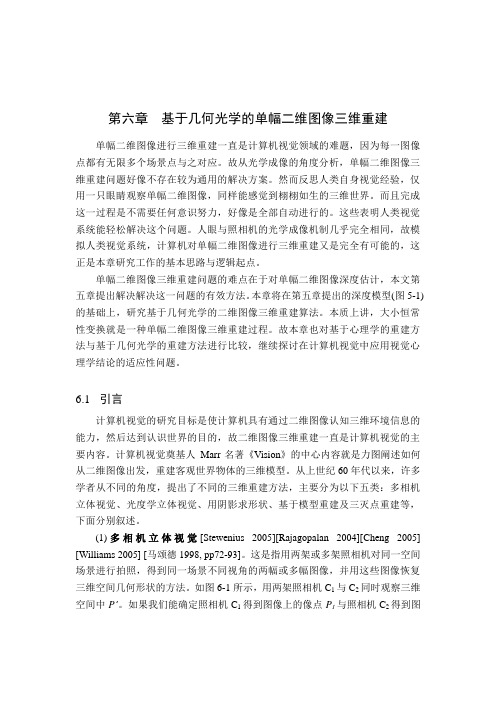
5.2 感知深度及模型在本章上述介绍的方法中，图像点的深度被定义为该图像点对应的场景点到相机光心(Pinhole)的距离。

实际上，这种对图像点深度的定义与人的感知习惯是不一致的。

根据视觉心理学理论与人们的日常体会，人类视觉基本上在无意识水平上运用三个规则来估计自我(Ego)与场景物体间的距离。

首先，人眼位于头上，而头又在身体上，身体由四肢支撑，四肢站在地面上[Gibson 1979, pp111, 205]。

这意味着，人眼在观察时离地面有一定的高度。

类似的，人们在照相时，相机光心(Pinhole)离地面也有一定的高度。

即使趴在地上照相，也是如此，因为相机本身具有一定的高度。

在本章的研究中，我们特别强调相机光心离地面的高度，这是第一条规则。

其次，人类视觉把人脚到物体脚之间的距离感知为物体的深度(脚到脚，foot-to-foot)，而不是人身体的其它部分到物体的其它部分的距离。

这是因为支持物体的地面是人类视觉深度感知最重要的参考面[Gibson 1979, pp156-164]。

例如，图5-1中的场景点P’, Q’有相同的深度，因为两点在同一竖线上，它们有相同的脚。

最后，如果在平坦地面上的直线与视网膜平面(即像平面，Imaging plane)平行，那么在这条直线上所有的点将会被感知有相同的深度。

这是因为当估计物体的距离时，人类视觉系统通常会调整或想象调整头或身体以保持眼睛正对着物体(面对面，Face-to -face) [Gibson 1979, pp111-126]。

例如，图5-1中直线L1与像平面Ⅱ平行，所以在L1上的点都与点P’有相同的深度。

这样，整个图像深度的估计便归结为垂直中轴线上各点的深度估计。

根据这些说明，我们把图像点的深度定义为遵守上述三条规则的、图像点对应场景点到相机光心的距离，而且称这种深度为感知深度(Perceived Depth, 缩写为PD)。

例如，图5-1中，图像点P的感知深度是场景点P’到点E(相机光心在地面的投影点)的物理距离。

这种定义与本文4.5.4中的实验结果是一致的。

现在给出本章使用的图像感知深度(PD)估计模型，见图5-1。

这个模型的输66第五章基于几何光学的单幅二维图像深度估计67入是单幅由被动视觉方法得到的二维图像；它的输出是图像垂直中轴线上各点的深度，这代表整个图像的深度；相机模型是考虑实际地面的针孔成像模型，在此模型中，相机离地面的高度是重要的深度感知因素；相机像平面被假定是与实际地面垂直的(后面的实验表明这个假定是不必要的)。

地面被假定是平的，这合乎人的感知经验[Gibson 1979, pp10,33,131]。

因为我们的目的仅是验证感知深度估计模型的有效性，所以对图像中的地面、物体等区域的分离都是手工进行的，因为图像分割技术目前还不是很成熟。

这个感知深度模型有很多实际应用，如移动机器人定位、基于计算机视觉的车辆自动导航和上一章的大小恒常性计算等。

在这些应用中，地面几乎是理想平坦的。

其实，日常生活中，平坦的视觉局部参考地面是处处存在的。

当我们观察桌子上的物品时，桌子就是参考地面。

当我们欣赏湖光水色时，水面就是理想参考地面。

当我们散步时，路面就是理想参考地面。

图5-1 考虑实际地面的相机针孔成像模型示意图（图像平面的比例被相对放大了）。

在此模型中，相机光心离地面的物理高度(h c )是重要的感知因素。

像平面（Image plane ）Ⅱ中的点U, P, Q 分别是场景点U ’, P ’, Q ’ 所对应的像点。

实际地平面Ⅰ被假定是理想平面。

通过场景点E , U ’, P ’ 的直线是相机光轴（Optical axis ）在地平面Ⅰ上的垂直投影，其中点E 是相机针孔 (Pinhole) O 在地平面Ⅰ上的垂直投影。

点P, P ’, U,U ’,Q,Q ’,E,A,V 与针孔O 共面，这个平面记作Ⅲ，它既垂直于平面Ⅰ又垂直于平面Ⅱ。

灭点（Vanishing point ）V 是相机光轴穿过相机图像平面Ⅱ所形成的交点，它一般位于平面Ⅱ的中心，即相机胶卷平面的中心。

像平面Ⅱ的中间线L 3把整个图像平面分成两部分：图像天空（Image sky ，下面部分）与图像地面（Image ground, 上面部分）。

h g 是图像地面的图像高度，h p 是图像点的图像高度（图像高度的概念在本章5.3介绍）。

z p 是的图像点P 感知深度（PD ）。

视觉心理学在计算机视觉中的应用研究5.3 基于几何光学的感知深度估计根据几何光学知识与图5-1中的成像模型，客观世界中位于实际天空与实际地面之间的地平线(灭线)，一定会沿着光轴投影到像平面Ⅱ上，并形成一条直线，记作L3。

该线也一定会与地面平行(见图5-1)。

如第四章4.2节所述，称L3为像平面的中间线，并称L3的中点为像平面的灭点(Vanishing point)，因为该点具有最大的感知深度。

L3也必然将像平面分成两部分：图像地面与图像天空，它们分别是由实际的地面与实际的天空投影形成的。

在本章中，我们仅计算图像地面的PD图，图像天空的PD图可用完全相同的方式来计算。

因为机械相机的胶片或数码相机的CCD图像传感器通常是矩形的，它们的尺寸是有限的，像平面顶部边界L4上点的PD在图像地面中是最小的，等于从场景点E到场景直线L2的距离，因为直线L2投影产生像平面顶部边界L4(见图5-1)。

所以我们称L4的中点U为像平面Ⅱ的近点(Closest point)，因在图像地面中点U的PD值最小。

按照PD的定义，像平面上位于同一行(水平线)上的像点的PD是相同的，所以计算整个图像地面的PD图便归结为计算线段UV上每一像点的PD。

设点P是线段UV上的任意一个像点，下面我们来推导点P的PD 的计算公式。

根据图5-1成像模型，像平面Ⅱ上的像点U, P, V，针孔O，及地平面Ⅰ上的场景点P’, U’, E是共面的，记作平面Ⅲ。

根据平面几何知识，三角形POV与三角形OP’E是相似的，即，△POV ∽△OP’E (5-1)我们把点P到中间线L3在图像平面上的距离称作图像高度(Image Height)，并记作h p(也即像平面Ⅱ上线段PV的长度，单位毫米)。

点P的PD(感知深度)是场景点P’到点E在实际地平面Ⅰ上的距离)，并记作z P (也即线段的P’E长度，单位米)。

从O到Ⅱ的距离记作f(也即线段OV的长度，单位毫米)。

从相机针孔O到地平面Ⅰ为相机高度记作h c (也即线段OE)的长度(单位米)。

因此，将这些记号代入式(5-1)，可得到下式：z p = h c×f / h p(5-2)68第五章基于几何光学的单幅二维图像深度估计然而，在图像中，h p通常使用像素单位(Pixel unit), 在此单位下，记它的值为h p-pixel。

不失一般性，设CCD传感器上每像素的高度是s毫米，s的单位是毫米/像素，则有h p = s×h p-pixel(5-3)现将式(5-3)代入式(5-2)，可得到z p = k / h p-pixel(5-4)这里k = h c×f /s对每一输入图像是一常量，所以z p能被1/h p-pixel唯一决定，这就是像点P的相对感知深度(PD)。

如图5-1所示，记整个图像地面的图像高度为h g，单位是像素。

不失一般性，可设输入图像是直立(即图像天空在图像的上部，而图像地面在图像的下部)，输入图像矩阵维数为m×n (宽×高)，单位为像素，坐标原点在图像矩阵的左上角。

同时设像点P的矩阵坐标为(p x , p y)，图像地面的图像高度记为h g，则有h p-pixel =|p y –n+h g|，代入式(5-4)，可得z p = k / | p y–n + h g|(5-5)因为像平面Ⅱ被假定是与实际地平面Ⅰ垂直的，而且CCD传感器通常在制造时是对称的，这就能保证灭点V与CCD传感器的中心位置对齐。