Maximun likelihood linear regression for speaker adaptation of
北京大学实证金融学讲义 7 volatility

• There are many types of non-linear models, e.g. - ARCH / GARCH - switching models - bilinear models
„Introductory Econometrics for Finance‟ © Chris Brooks 2002
• What could the current value of the variance of the errors plausibly depend upon? – Previous squared error terms. • This leads to the autoregressive conditionally heteroscedastic model for the variance of the errors: t2 = 0 + 1 u2 t 1 • This is known as an ARCH(1) model.
„Introductory Econometrics for Finance‟ © Chris Brooks 2002
2
A Sample Financial Asset Returns Time Series
Daily S&P 500 Returns for January 1990 – December 1999
• Campbell, Lo and MacKinlay (1997) define a non-linear data generating process as one that can be written yt = f(ut, ut-1, ut-2, …) where ut is an iid error term and f is a non-linear function. • They also give a slightly more specific definition as yt = g(ut-1, ut-2, …)+ ut2(ut-1, ut-2, …) where g is a function of past error terms only and 2 is a variance term. • Models with nonlinear g(•) are “non-linear in mean”, while those with nonlinear 2(•) are “non-linear in variance”.
计量经济学英语专业词汇

• • • •
•
• • • •
模型设定正确假设。The regression model is correctly specified. 线性回归假设。The regression model is linear in the parameters。 与随机项不相关假设。The covariances between Xi and μi are zero. 观测值变化假设。X values in a given sample must not all be the same. 无完全共线性假设。There is no perfect multicollinearity among the explanatory variables. 0均值假设。The conditional mean value of μi is zero. 同方差假设。The conditional variances of μi are identical.(Homoscedasticity) 序列不相关假设。The correlation between any two μi and μj is zero. 正态性假设。The μ’s follow the normal distribution.
• 方程的显著性检验(F检验) Testing the Overall Significance of a Multiple Regression (the F test) • 假设检验(Hypothesis Testing)变量的显著性检验(t检 验) Testing the Significance of Variables (the t test) • 参数的置信区间 Confidence Interval of Parameter • 置信系数(置信度)(confidence coefficient) • 置信限(confidence limit) • 恩格尔曲线(Engle curves) • 菲利普斯曲线(Pillips cuves)
AI术语

人工智能专业重要词汇表1、A开头的词汇:Artificial General Intelligence/AGI通用人工智能Artificial Intelligence/AI人工智能Association analysis关联分析Attention mechanism注意力机制Attribute conditional independence assumption属性条件独立性假设Attribute space属性空间Attribute value属性值Autoencoder自编码器Automatic speech recognition自动语音识别Automatic summarization自动摘要Average gradient平均梯度Average-Pooling平均池化Accumulated error backpropagation累积误差逆传播Activation Function激活函数Adaptive Resonance Theory/ART自适应谐振理论Addictive model加性学习Adversarial Networks对抗网络Affine Layer仿射层Affinity matrix亲和矩阵Agent代理/ 智能体Algorithm算法Alpha-beta pruningα-β剪枝Anomaly detection异常检测Approximation近似Area Under ROC Curve/AUC R oc 曲线下面积2、B开头的词汇Backpropagation Through Time通过时间的反向传播Backpropagation/BP反向传播Base learner基学习器Base learning algorithm基学习算法Batch Normalization/BN批量归一化Bayes decision rule贝叶斯判定准则Bayes Model Averaging/BMA贝叶斯模型平均Bayes optimal classifier贝叶斯最优分类器Bayesian decision theory贝叶斯决策论Bayesian network贝叶斯网络Between-class scatter matrix类间散度矩阵Bias偏置/ 偏差Bias-variance decomposition偏差-方差分解Bias-Variance Dilemma偏差–方差困境Bi-directional Long-Short Term Memory/Bi-LSTM双向长短期记忆Binary classification二分类Binomial test二项检验Bi-partition二分法Boltzmann machine玻尔兹曼机Bootstrap sampling自助采样法/可重复采样/有放回采样Bootstrapping自助法Break-Event Point/BEP平衡点3、C开头的词汇Calibration校准Cascade-Correlation级联相关Categorical attribute离散属性Class-conditional probability类条件概率Classification and regression tree/CART分类与回归树Classifier分类器Class-imbalance类别不平衡Closed -form闭式Cluster簇/类/集群Cluster analysis聚类分析Clustering聚类Clustering ensemble聚类集成Co-adapting共适应Coding matrix编码矩阵COLT国际学习理论会议Committee-based learning基于委员会的学习Competitive learning竞争型学习Component learner组件学习器Comprehensibility可解释性Computation Cost计算成本Computational Linguistics计算语言学Computer vision计算机视觉Concept drift概念漂移Concept Learning System /CLS概念学习系统Conditional entropy条件熵Conditional mutual information条件互信息Conditional Probability Table/CPT条件概率表Conditional random field/CRF条件随机场Conditional risk条件风险Confidence置信度Confusion matrix混淆矩阵Connection weight连接权Connectionism连结主义Consistency一致性/相合性Contingency table列联表Continuous attribute连续属性Convergence收敛Conversational agent会话智能体Convex quadratic programming凸二次规划Convexity凸性Convolutional neural network/CNN卷积神经网络Co-occurrence同现Correlation coefficient相关系数Cosine similarity余弦相似度Cost curve成本曲线Cost Function成本函数Cost matrix成本矩阵Cost-sensitive成本敏感Cross entropy交叉熵Cross validation交叉验证Crowdsourcing众包Curse of dimensionality维数灾难Cut point截断点Cutting plane algorithm割平面法4、D开头的词汇Data mining数据挖掘Data set数据集Decision Boundary决策边界Decision stump决策树桩Decision tree决策树/判定树Deduction演绎Deep Belief Network深度信念网络Deep Convolutional Generative Adversarial Network/DCGAN深度卷积生成对抗网络Deep learning深度学习Deep neural network/DNN深度神经网络Deep Q-Learning深度Q 学习Deep Q-Network深度Q 网络Density estimation密度估计Density-based clustering密度聚类Differentiable neural computer可微分神经计算机Dimensionality reduction algorithm降维算法Directed edge有向边Disagreement measure不合度量Discriminative model判别模型Discriminator判别器Distance measure距离度量Distance metric learning距离度量学习Distribution分布Divergence散度Diversity measure多样性度量/差异性度量Domain adaption领域自适应Downsampling下采样D-separation (Directed separation)有向分离Dual problem对偶问题Dummy node哑结点Dynamic Fusion动态融合Dynamic programming动态规划5、E开头的词汇Eigenvalue decomposition特征值分解Embedding嵌入Emotional analysis情绪分析Empirical conditional entropy经验条件熵Empirical entropy经验熵Empirical error经验误差Empirical risk经验风险End-to-End端到端Energy-based model基于能量的模型Ensemble learning集成学习Ensemble pruning集成修剪Error Correcting Output Codes/ECOC纠错输出码Error rate错误率Error-ambiguity decomposition误差-分歧分解Euclidean distance欧氏距离Evolutionary computation演化计算Expectation-Maximization期望最大化Expected loss期望损失Exploding Gradient Problem梯度爆炸问题Exponential loss function指数损失函数Extreme Learning Machine/ELM超限学习机6、F开头的词汇Factorization因子分解False negative假负类False positive假正类False Positive Rate/FPR假正例率Feature engineering特征工程Feature selection特征选择Feature vector特征向量Featured Learning特征学习Feedforward Neural Networks/FNN前馈神经网络Fine-tuning微调Flipping output翻转法Fluctuation震荡Forward stagewise algorithm前向分步算法Frequentist频率主义学派Full-rank matrix满秩矩阵Functional neuron功能神经元7、G开头的词汇Gain ratio增益率Game theory博弈论Gaussian kernel function高斯核函数Gaussian Mixture Model高斯混合模型General Problem Solving通用问题求解Generalization泛化Generalization error泛化误差Generalization error bound泛化误差上界Generalized Lagrange function广义拉格朗日函数Generalized linear model广义线性模型Generalized Rayleigh quotient广义瑞利商Generative Adversarial Networks/GAN生成对抗网络Generative Model生成模型Generator生成器Genetic Algorithm/GA遗传算法Gibbs sampling吉布斯采样Gini index基尼指数Global minimum全局最小Global Optimization全局优化Gradient boosting梯度提升Gradient Descent梯度下降Graph theory图论Ground-truth真相/真实8、H开头的词汇Hard margin硬间隔Hard voting硬投票Harmonic mean调和平均Hesse matrix海塞矩阵Hidden dynamic model隐动态模型Hidden layer隐藏层Hidden Markov Model/HMM隐马尔可夫模型Hierarchical clustering层次聚类Hilbert space希尔伯特空间Hinge loss function合页损失函数Hold-out留出法Homogeneous同质Hybrid computing混合计算Hyperparameter超参数Hypothesis假设Hypothesis test假设验证9、I开头的词汇ICML国际机器学习会议Improved iterative scaling/IIS改进的迭代尺度法Incremental learning增量学习Independent and identically distributed/i.i.d.独立同分布Independent Component Analysis/ICA独立成分分析Indicator function指示函数Individual learner个体学习器Induction归纳Inductive bias归纳偏好Inductive learning归纳学习Inductive Logic Programming/ILP归纳逻辑程序设计Information entropy信息熵Information gain信息增益Input layer输入层Insensitive loss不敏感损失Inter-cluster similarity簇间相似度International Conference for Machine Learning/ICML国际机器学习大会Intra-cluster similarity簇内相似度Intrinsic value固有值Isometric Mapping/Isomap等度量映射Isotonic regression等分回归Iterative Dichotomiser迭代二分器10、K开头的词汇Kernel method核方法Kernel trick核技巧Kernelized Linear Discriminant Analysis/KLDA核线性判别分析K-fold cross validation k 折交叉验证/k 倍交叉验证K-Means Clustering K –均值聚类K-Nearest Neighbours Algorithm/KNN K近邻算法Knowledge base知识库Knowledge Representation知识表征11、L开头的词汇Label space标记空间Lagrange duality拉格朗日对偶性Lagrange multiplier拉格朗日乘子Laplace smoothing拉普拉斯平滑Laplacian correction拉普拉斯修正Latent Dirichlet Allocation隐狄利克雷分布Latent semantic analysis潜在语义分析Latent variable隐变量Lazy learning懒惰学习Learner学习器Learning by analogy类比学习Learning rate学习率Learning Vector Quantization/LVQ学习向量量化Least squares regression tree最小二乘回归树Leave-One-Out/LOO留一法linear chain conditional random field线性链条件随机场Linear Discriminant Analysis/LDA线性判别分析Linear model线性模型Linear Regression线性回归Link function联系函数Local Markov property局部马尔可夫性Local minimum局部最小Log likelihood对数似然Log odds/logit对数几率Logistic Regression Logistic 回归Log-likelihood对数似然Log-linear regression对数线性回归Long-Short Term Memory/LSTM长短期记忆Loss function损失函数12、M开头的词汇Machine translation/MT机器翻译Macron-P宏查准率Macron-R宏查全率Majority voting绝对多数投票法Manifold assumption流形假设Manifold learning流形学习Margin theory间隔理论Marginal distribution边际分布Marginal independence边际独立性Marginalization边际化Markov Chain Monte Carlo/MCMC马尔可夫链蒙特卡罗方法Markov Random Field马尔可夫随机场Maximal clique最大团Maximum Likelihood Estimation/MLE极大似然估计/极大似然法Maximum margin最大间隔Maximum weighted spanning tree最大带权生成树Max-Pooling最大池化Mean squared error均方误差Meta-learner元学习器Metric learning度量学习Micro-P微查准率Micro-R微查全率Minimal Description Length/MDL最小描述长度Minimax game极小极大博弈Misclassification cost误分类成本Mixture of experts混合专家Momentum动量Moral graph道德图/端正图Multi-class classification多分类Multi-document summarization多文档摘要Multi-layer feedforward neural networks多层前馈神经网络Multilayer Perceptron/MLP多层感知器Multimodal learning多模态学习Multiple Dimensional Scaling多维缩放Multiple linear regression多元线性回归Multi-response Linear Regression /MLR多响应线性回归Mutual information互信息13、N开头的词汇Naive bayes朴素贝叶斯Naive Bayes Classifier朴素贝叶斯分类器Named entity recognition命名实体识别Nash equilibrium纳什均衡Natural language generation/NLG自然语言生成Natural language processing自然语言处理Negative class负类Negative correlation负相关法Negative Log Likelihood负对数似然Neighbourhood Component Analysis/NCA近邻成分分析Neural Machine Translation神经机器翻译Neural Turing Machine神经图灵机Newton method牛顿法NIPS国际神经信息处理系统会议No Free Lunch Theorem/NFL没有免费的午餐定理Noise-contrastive estimation噪音对比估计Nominal attribute列名属性Non-convex optimization非凸优化Nonlinear model非线性模型Non-metric distance非度量距离Non-negative matrix factorization非负矩阵分解Non-ordinal attribute无序属性Non-Saturating Game非饱和博弈Norm范数Normalization归一化Nuclear norm核范数Numerical attribute数值属性14、O开头的词汇Objective function目标函数Oblique decision tree斜决策树Occam’s razor奥卡姆剃刀Odds几率Off-Policy离策略One shot learning一次性学习One-Dependent Estimator/ODE独依赖估计On-Policy在策略Ordinal attribute有序属性Out-of-bag estimate包外估计Output layer输出层Output smearing输出调制法Overfitting过拟合/过配Oversampling过采样15、P开头的词汇Paired t-test成对t 检验Pairwise成对型Pairwise Markov property成对马尔可夫性Parameter参数Parameter estimation参数估计Parameter tuning调参Parse tree解析树Particle Swarm Optimization/PSO粒子群优化算法Part-of-speech tagging词性标注Perceptron感知机Performance measure性能度量Plug and Play Generative Network即插即用生成网络Plurality voting相对多数投票法Polarity detection极性检测Polynomial kernel function多项式核函数Pooling池化Positive class正类Positive definite matrix正定矩阵Post-hoc test后续检验Post-pruning后剪枝potential function势函数Precision查准率/准确率Prepruning预剪枝Principal component analysis/PCA主成分分析Principle of multiple explanations多释原则Prior先验Probability Graphical Model概率图模型Proximal Gradient Descent/PGD近端梯度下降Pruning剪枝Pseudo-label伪标记16、Q开头的词汇Quantized Neural Network量子化神经网络Quantum computer量子计算机Quantum Computing量子计算Quasi Newton method拟牛顿法17、R开头的词汇Radial Basis Function/RBF径向基函数Random Forest Algorithm随机森林算法Random walk随机漫步Recall查全率/召回率Receiver Operating Characteristic/ROC受试者工作特征Rectified Linear Unit/ReLU线性修正单元Recurrent Neural Network循环神经网络Recursive neural network递归神经网络Reference model参考模型Regression回归Regularization正则化Reinforcement learning/RL强化学习Representation learning表征学习Representer theorem表示定理reproducing kernel Hilbert space/RKHS再生核希尔伯特空间Re-sampling重采样法Rescaling再缩放Residual Mapping残差映射Residual Network残差网络Restricted Boltzmann Machine/RBM受限玻尔兹曼机Restricted Isometry Property/RIP限定等距性Re-weighting重赋权法Robustness稳健性/鲁棒性Root node根结点Rule Engine规则引擎Rule learning规则学习18、S开头的词汇Saddle point鞍点Sample space样本空间Sampling采样Score function评分函数Self-Driving自动驾驶Self-Organizing Map/SOM自组织映射Semi-naive Bayes classifiers半朴素贝叶斯分类器Semi-Supervised Learning半监督学习semi-Supervised Support Vector Machine半监督支持向量机Sentiment analysis情感分析Separating hyperplane分离超平面Sigmoid function Sigmoid 函数Similarity measure相似度度量Simulated annealing模拟退火Simultaneous localization and mapping同步定位与地图构建Singular Value Decomposition奇异值分解Slack variables松弛变量Smoothing平滑Soft margin软间隔Soft margin maximization软间隔最大化Soft voting软投票Sparse representation稀疏表征Sparsity稀疏性Specialization特化Spectral Clustering谱聚类Speech Recognition语音识别Splitting variable切分变量Squashing function挤压函数Stability-plasticity dilemma可塑性-稳定性困境Statistical learning统计学习Status feature function状态特征函Stochastic gradient descent随机梯度下降Stratified sampling分层采样Structural risk结构风险Structural risk minimization/SRM结构风险最小化Subspace子空间Supervised learning监督学习/有导师学习support vector expansion支持向量展式Support Vector Machine/SVM支持向量机Surrogat loss替代损失Surrogate function替代函数Symbolic learning符号学习Symbolism符号主义Synset同义词集19、T开头的词汇T-Distribution Stochastic Neighbour Embedding/t-SNE T–分布随机近邻嵌入Tensor张量Tensor Processing Units/TPU张量处理单元The least square method最小二乘法Threshold阈值Threshold logic unit阈值逻辑单元Threshold-moving阈值移动Time Step时间步骤Tokenization标记化Training error训练误差Training instance训练示例/训练例Transductive learning直推学习Transfer learning迁移学习Treebank树库Tria-by-error试错法True negative真负类True positive真正类True Positive Rate/TPR真正例率Turing Machine图灵机Twice-learning二次学习20、U开头的词汇Underfitting欠拟合/欠配Undersampling欠采样Understandability可理解性Unequal cost非均等代价Unit-step function单位阶跃函数Univariate decision tree单变量决策树Unsupervised learning无监督学习/无导师学习Unsupervised layer-wise training无监督逐层训练Upsampling上采样21、V开头的词汇Vanishing Gradient Problem梯度消失问题Variational inference变分推断VC Theory VC维理论Version space版本空间Viterbi algorithm维特比算法Von Neumann architecture冯·诺伊曼架构22、W开头的词汇Wasserstein GAN/WGAN Wasserstein生成对抗网络Weak learner弱学习器Weight权重Weight sharing权共享Weighted voting加权投票法Within-class scatter matrix类内散度矩阵Word embedding词嵌入Word sense disambiguation词义消歧23、Z开头的词汇Zero-data learning零数据学习Zero-shot learning零次学习。
最大似然估计(Maximum likelihood estimation)(通过例子理解)

最大似然估计(Maximum likelihood estimation)(通过例子理解)之前看书上的一直不理解到底什么是似然,最后还是查了好几篇文章后才明白,现在我来总结一下吧,要想看懂最大似然估计,首先我们要理解什么是似然,不然对我来说不理解似然,我就一直在困惑最大似然估计到底要求的是个什么东西,而那个未知数θ到底是个什么东西TT似然与概率在统计学中,似然函数(likelihood function,通常简写为likelihood,似然)是一个非常重要的内容,在非正式场合似然和概率(Probability)几乎是一对同义词,但是在统计学中似然和概率却是两个不同的概念。
概率是在特定环境下某件事情发生的可能性,也就是结果没有产生之前依据环境所对应的参数来预测某件事情发生的可能性,比如抛硬币,抛之前我们不知道最后是哪一面朝上,但是根据硬币的性质我们可以推测任何一面朝上的可能性均为50%,这个概率只有在抛硬币之前才是有意义的,抛完硬币后的结果便是确定的;而似然刚好相反,是在确定的结果下去推测产生这个结果的可能环境(参数),还是抛硬币的例子,假设我们随机抛掷一枚硬币1,000次,结果500次人头朝上,500次数字朝上(实际情况一般不会这么理想,这里只是举个例子),我们很容易判断这是一枚标准的硬币,两面朝上的概率均为50%,这个过程就是我们根据结果来判断这个事情本身的性质(参数),也就是似然。
结果和参数相互对应的时候,似然和概率在数值上是相等的,如果用θ 表示环境对应的参数,x 表示结果,那么概率可以表示为:P(x|θ)P(x|θ)是条件概率的表示方法,θ是前置条件,理解为在θ 的前提下,事件 x 发生的概率,相对应的似然可以表示为:理解为已知结果为 x ,参数为θ (似然函数里θ 是变量,这里## 标题 ##说的参数是相对与概率而言的)对应的概率,即:需要说明的是两者在数值上相等,但是意义并不相同,是关于θ 的函数,而 P 则是关于 x 的函数,两者从不同的角度描述一件事情。
医学统计学名词解释精心整理(带英文)

同质 (Homogeneity):医学研究对象具有的某种共性。
变异 (Variation) :同质研究对象变量值之间的差异。
总体 (Population):根据研究目的确定的所有同质的观察单位某项观测值的全体称为总体。
样本 (Sample):来自于总体的部分观察单位的观测值称为样本。
参数 (Parameter):由总体中全部观测值所计算出的反映总体特征的统计指标。
统计量 (Statistic):由样本观测值所计算出的反映样本特征的统计指标。
变量 (Variable) :指观察单位的某项特征。
它能表现观察单位的变异性。
概率 (Probability):是随机事件发生可能性大小,用P表示,其取值为[0,1]。
频率 (Frequency) :在相同的条件下,独立地重复做n次试验,随机事件A出现m次,则比值m/n为随机事件A出现的频率。
随机误差 (Random error):是由于一系列实验或观察条件等因素的随机波动造成的测量值与真实值之间的差异。
随机误差是不可避免的,且大小和方向都不固定。
抽样误差 (Sampling error):由个体变异产生、随机抽样造成的若干个样本统计量之间以及样本统计量与总体参数之间的差异称为抽样误差。
系统误差 (Systematic error) :实际观测中,由于仪器未校正,测量者感官的某种偏差,医生掌握疗效标准偏高或偏低等,而使观测值有方向性、系统性或周期性地偏离真值。
四分位数间距 (Quartile range) :上四分位数与下四分位数的差值,用Q表示。
通常用来描述偏态分布资料的离散趋势。
变异系数 (Coefficient of variation) CV :是标准差与均数之比,用于比较测量单位不同或均数相差较大的两组或以上数据的离散程度。
参考值范围 (Reference range) :绝大多数“正常人”的解剖、生理、生化等某项指标的波动范围。
构成比 (Proportion) :表示事物内部某一组成部分观察单位数与该事物各组成部分的观察单位总数之比,用以说明事物内部各组成部分所占的比重。
计量经济学课后试验 7和17章
C7.4(i)The two signs that are pretty clear are β3< 0 (because hsperc is defined so that the smaller the number the better the student) and β4 > 0. The effect of size of graduating class is not clear. It is also unclear whether males and females have systematically different GPAs. We may think that β6 < 0, that is, athletes do worse than other students with comparable characteristics. But remember, we are controlling for ability to some degree with hsperc and sat.有两个系数是可以确定的,β3< 0(因为hsperc学生的成绩排名被定义的是:越小成绩越好);β4 > 0(SAT考试,分数越高成绩越好)。
班上的人数对colgpa的影响不明确。
性别在colgpa 的区别上也不明确。
我们可以认为β6 < 0,也就是说运动员比其他学生的colgpa小。
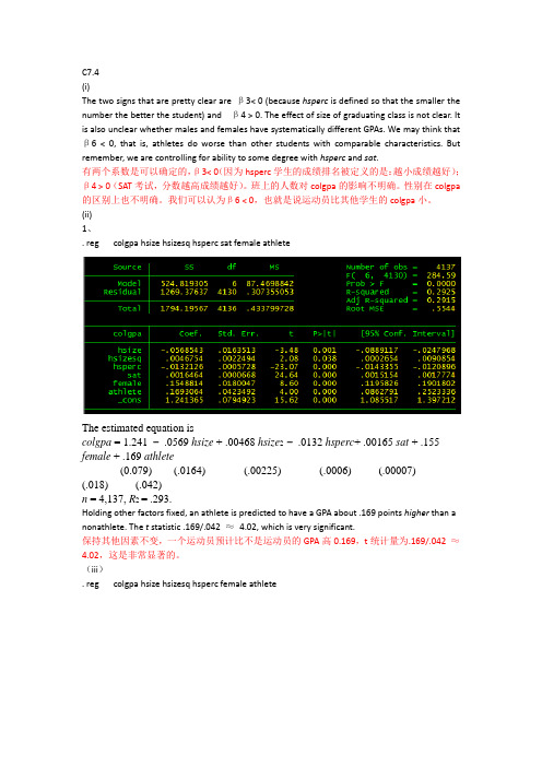
(ii)1、. reg colgpa hsize hsizesq hsperc sat female athleteThe estimated equation iscolgpa = 1.241 −.0569 hsize + .00468 hsize2 −.0132 hsperc+ .00165 sat + .155 female + .169 athlete(0.079) (.0164) (.00225) (.0006) (.00007)(.018) (.042)n = 4,137, R2 = .293.Holding other factors fixed, an athlete is predicted to have a GPA about .169 points higher than a nonathlete. The t statistic .169/.042 ≈4.02, which is very significant.保持其他因素不变,一个运动员预计比不是运动员的GPA高0.169,t统计量为.169/.042 ≈4.02,这是非常显著的。
mllr

2.1. Spectral Mapping Approach
The spectral mapping approach is based on the belief that a recognition system can be improved by matching the new speaker’s features vectors to the vectors of the training data [5]. The mapping is designed so that the difference between the reference vector set and the mapped vector set is minimized. These differences are due to the spectral differences of the speakers’ speech production systems (e.g. vocal tract length and shape). Initial attempts at spectral mapping adaptation were used in the spectral template matching systems [6, 7, 8]. These consider the template to be from the reference speaker and automatically generate a transformation to minimize the difference between the new speaker and the reference speaker [5]. Other approaches [9] have mapped both the reference data and the new speaker’s data into a common vector set which is said to maximally correlate the two. A variation on these methods which is similar to speaker normalization uses a transform to map each speaker in the speaker-independent training set onto a reference speaker [10, 11]. Thus, the models generated act as speaker-dependent models. This approach is illustrated in Figure 2 and is commonly referred to as a speaker normalization technique.
极大似然估计案例

ML ESTIMATION IN STATAMany estimation procedures in Stata are based on the principle of Maximum Likelihood. For a lot of common estimators knowledge of ML is not strictly necessary (linear regression with OLS, 2SLS, SUR) since their matrix derivation gives the same result as the ML outcome. However, there are also techniques that explicitly make use of ML. Examples are non-linear binary choice models (e.g. Logit, Probit, Multinomial Logit), models for time-series data (e.g. ARIMA) and binary choice models for panel data (fixed effects logit model).The flexibility of Stata is mainly due to the fact that all procedures (estimators, tests, basic statistics but also graphs) are programmed in so-called ado -files. You can also program your own ado-files if Stata doesn’t support an estimator or test that you need for your research. Of course, this requires knowledge on programming in Stata.Using ML in Stata also requires that you write your own (small) programs for your particular problem. In short there are a number of steps to go through in order to do ML estimation in Stata:1. Derive the log-likelihood function from your probability model. This is done on paper and is of course dependent on the assumptions you make on the distribution underlying the data (e.g. normal or logistic).2. Write a program that calculates the log-likelihood values and, optionally for difficult models, its derivatives in an ado -file. This program is known as a likelihood evaluator3. Identify a particular model to fit using your data variables and the ml model statement4. Fit the model using ml maximize .Let’s go through these steps for a well-known non-linear model, the logit model. In a logit model the dependent variable typically has only two values, 0 or 1. Applications are consumer choice behavior, investment decisions etc. In this example we try to explain why some farmers have chosen organic farming and other not. A dataset with 473 observations on dairy farmers in the period 1994-1999 is available. The following variables are available.Variable Description and unitsbiodum 1 if organic farmer, 0 if conventional farmerage yearssucc 1 if there is a successor, 0 if nottenure 1 if more than half of the land is rented, 0 if notclay 1 if major soil type is clay, 0 if noteduc 1 if farmer has higher education, 0 otherwisesizequo dairy production quota in 100,000 kgsizeha acreage in hectaresanimalha number of animals per haprof profits in 100,000 Euros1. Derive the log-likelihood function from your probability model.()1Pr =y is defined by the expression for the density function of the logistic distribution that underlies the logit model. So, ()()Xb e y −+==111Pr . Since we only observe values 1 or 0 for the variable biodum we can also define an expression for ()0Pr =y : ()()()()()()XbXb Xb Xb XbXb e e e e e e y −−−−−−+=+−++=+−==111111110Pr This leads to the following definition of the loglikelihood for the j th observation in the logit model:()()()()()()()()()=+−−=+−=+=+−=+−=+=−−−−−−−−01ln 1ln ln 1ln 11ln 1ln )1ln(11ln ln i Xb Xb Xb Xb Xb i Xb Xb Xb j y if e Xb e e e ey if e e e l2. Write a program (Stata ado file) that calculates the log-likelihood valuesprogram define mylogitargs lnf Xbquietly replace `lnf' = -ln(1+exp(-`Xb')) if $ML_y1==1 quietly replace `lnf' = -`Xb' -ln(1+exp(-`Xb')) if $ML_y1==0 end3. Identify a particular model to fit using your data variables and the ml model statementml model lf mylogit (biodum = age succ tenure clay educ sizeha sizequo animalha prof)4. Fit the model using ml maximize .. ml maximizeinitial: log likelihood = -327.85862alternative: log likelihood = -284.23841rescale: log likelihood = -268.17278Iteration 0: log likelihood = -268.17278Iteration 1: log likelihood = -185.84208Iteration 2: log likelihood = -161.98223Iteration 3: log likelihood = -159.3928Iteration 4: log likelihood = -159.37492Iteration 5: log likelihood = -159.37492Number of obs = 473 Wald chi2(9) = 95.39 Log likelihood = -159.37492 Prob > chi2 = 0.0000------------------------------------------------------------------------------ biodum | Coef. Std. Err. z P>|z| [95% Conf. Interval] -------------+---------------------------------------------------------------- age | -.0271121 .0161332 -1.68 0.093 -.0587326 .0045085 succ | -.3254785 .438487 -0.74 0.458 -1.184897 .5339403 tenure | -.3761036 .5109148 -0.74 0.462 -1.377478 .6252709 clay | .2660545 .3076138 0.86 0.387 -.3368576 .8689665 educ | 2.66085 .4142379 6.42 0.000 1.848958 3.472741 sizeha | -.0195829 .0141403 -1.38 0.166 -.0472974 .0081316 sizequo | -.3481513 .1456595 -2.39 0.017 -.6336387 -.062664 animalha | -3.351957 .4730748 -7.09 0.000 -4.279167 -2.424748 prof | .6485803 .2552814 2.54 0.011 .148238 1.148923 _cons | 6.221396 1.235341 5.04 0.000 3.800171 8.64262These results are exactly the same as the one we would get using the logit command available in Stata.The results already give the outcome for a Wald test of H 0 : 0====prof succ age βββK . We could test other hypotheses using the straightforward LR test. E.g to test whether personal characteristics matter we can test the null hypothesis 0===educ succ age βββ. Estimate the model again with these three variables omitted:Identify the new model to fit using your data variables and the ml model statementml model lf mylogit (biodum = tenure clay sizeha sizequo animalha prof)ml maximizeNumber of obs = 473 Wald chi2(6) = 79.64 Log likelihood = -195.21467 Prob > chi2 = 0.0000 ------------------------------------------------------------------------------ biodum | Coef. Std. Err. z P>|z| [95% Conf. Interval] -------------+---------------------------------------------------------------- tenure | .7022649 .4007155 1.75 0.080 -.0831231 1.487653 clay | -.0454245 .2667705 -0.17 0.865 -.5682852 .4774362 sizeha | .0052992 .0123222 0.43 0.667 -.0188519 .0294504 sizequo | -.3474167 .14042 -2.47 0.013 -.6226347 -.0721986 animalha | -2.390138 .39364 -6.07 0.000 -3.161658 -1.618618 prof | .3865246 .2174228 1.78 0.075 -.0396164 .8126655 _cons | 3.871129 .8605505 4.50 0.000 2.184481 5.557777The LR test statistic is []()81.7368.7121.19537.15922=>=−−−=χLR so we firmly reject this null hypothesis.We could have tested this with an LM test. Then we need to create cross-products of the residuals ε with x and z. First, residuals ε were created based on the estimated model. Using the estimated ML model, we made predictions and then took the difference with the observed valuesgen e=biodum-biodumfNext, the cross products 'ˆi i x εand 'ˆi i z ε were created where the vector z i contains the omitted variable age , educ, and succ:gen e_age=e*agegen e_succ=e*succgen e_tenure=e*tenuregen e_clay=e*claygen e_educ=e*educgen e_sizeha=e*sizehagen e_sizequo=e*sizequogen e_animalh=e*animalhgen e_prof=e*profWe can do the LM test in a straightforward fashion by estimating the following equation without intercept!u prof succ age +⋅++⋅+⋅=εεε (1)So, create a vector of ones:gen ones=1reg ones e_age e_succ e_tenure e_clay e_educ e_sizeha e_sizequo e_animalh e_prof, noconstantSource | SS df MS Number of obs = 473 -------------+------------------------------ F( 9, 464) = 8.96 Model | 70.0368282 9 7.7818698 Prob > F = 0.0000 Residual | 402.963172 464 .868455112 R-squared = 0.1481 -------------+------------------------------ Adj R-squared = 0.1315 Total | 473 473 1 Root MSE = .93191------------------------------------------------------------------------------ ones | Coef. Std. Err. t P>|t| [95% Conf. Interval] -------------+---------------------------------------------------------------- e_age | -.0065348 .011938 -0.55 0.584 -.0299941 .0169245 e_succ | -.1558425 .3272642 -0.48 0.634 -.798946 .487261 e_tenure | -.3956457 .4480105 -0.88 0.378 -1.276027 .4847352 e_clay | .4048804 .2566723 1.58 0.115 -.0995037 .9092644 e_educ | 2.495919 .3029164 8.24 0.000 1.900661 3.091177 e_sizeha | -.0006441 .0108471 -0.06 0.953 -.0219597 .0206714 e_sizequo | -.3132451 .1293209 -2.42 0.016 -.5673724 -.0591179 e_animalh | -.1441578 .3363157 -0.43 0.668 -.8050484 .5167328 e_prof | .1131073 .2338385 0.48 0.629 -.3464064 .5726209 ------------------------------------------------------------------------------Finally we can obtain the LM test statistic NR 2 = 473*0.148 = 70.04 ()81.732=>χThe LM test statistic is close to the test value of the LR value and it holds that LM LR ξξ≥.。
- 1、下载文档前请自行甄别文档内容的完整性,平台不提供额外的编辑、内容补充、找答案等附加服务。
- 2、"仅部分预览"的文档,不可在线预览部分如存在完整性等问题,可反馈申请退款(可完整预览的文档不适用该条件!)。
- 3、如文档侵犯您的权益,请联系客服反馈,我们会尽快为您处理(人工客服工作时间:9:00-18:30)。
• Consider the case of a continuous density HMM system with Gaussian output distributions.
• A particular distribution s ,is characterized by a mean vector s ,
data, a transformation may still be applied (global transformation)
6
Estimation of MLLR regression matrices
• 1.Definition of auxiliary function
S
– Assume the adaptation data, O, is a series of T observations.
and a covariance matrix C s
• Given a parameterized speech frame vector o , the probability
density of that vector being generated by distribution s is bs o
j 1
T j t log2 n / 2
t 1
log C j
1/ 2
1 2
ot
j
' C j 1
ot
j
S
constant FO |
j 1
T t 1
j
t
1 2
n
log2
1 2
log
C
j
1 2
ot
j
' C j 1
ot
j
constant
1 2
F O
|
S j 1
T t 1
(Maximum - Likelihood)
Q , E log F O, | | O,
E-step
FO, | log F O, |
V
7
Estimation of MLLR regression matrices (cont.)
• 2.Maximization of auxiliary function
FO | T
s tCs1 ot Wss
s'
t1
0
hence
T
T
s t Cs1ots' s t Cs1Wsss'
<= 估測 W s 的general form
(5)
t 1
t 1
11
Estimation of MLLR regression matrices (cont.)
j tnlog2 log Cj
ot
W
j j
' C j 1
ot
W
j j
1 FO | d
2
dW s
S j1
T
j tnlog2 log Cj
t 1
ot W
j j
'
C
1 j
ot
W
j
j
1 2
FO | T s t*2*Cs1 *
t1
ot
W s s
*
s'
X T AX 2 AX X
s [, 1, 2 ,..., n ]'
offset = 1, include an offset in the regression
offset = 0, ignore offsets
若調適語者的錄音環境與初始模型錄音環境不同時, 可以加入的一項參數 [參考資料]
• So the probability density function for the adapted system becomes
s t
F
1
O
|
V
F
O,
t
s |
8
Estimation of MLLR regression matrices (cont.)
• 2.Maximization of auxiliary function (cont.)
已知 s t
F
1
O
|
V
F
O,
t
s |
則
T
Q , constant F O, | log bt ot V t 1
1 1/ 2oWss ' Cs1 oWss
b o e s
n/ 2 1/ 2
2 Cs
(1)
5
MLLR’s adaptation approach (cont.)
• The transformation matrices Ws are calculated to maximize the
likelihood of the adaptation data • The transformation matrices can be implemented using the
where n is the dimension of the observation vector
S
bs o 2
1 1/ 2os ' Cs1 os e n / 2 1/ 2
Cs
speech frame vector
4
MLLR’s adaptation approach (cont.)
– The totallikelihood of the modelset generate the observation sequenceis
FO | FO, |
objective function V
– Define an auxiliary function,and We want tomaximize it
(3)
V t 1
- Defines S as theset of all statedistributions in the system
and s t as the a posterioriprobability of occupyingstate s at timet
given that the observation sequence O is generated
• The other HMM parameters are not adapted since the main differences between speakers are assumed to be characterized by the means
3
MLLR’s adaptation approach (cont.)
Q , E log F O, | | O,
FO, | log F O, | V
F O, | V
log 1 b1
o1
T
a b t 1t t
t2
ot
(2)
only related with mean
T
constant F O, | log bt ot
forward–backward algorithm • A more general approach is adopted in which the same
transformations matrix is used for several distributions. • If some of the distributions are not observed in the adaptation
Present by Hsu Ting-Wei 2006.03.16
Introduction
Speaker
HMM Models
Say: “Hello!”
• Speaker adaptation techniques fall into two main categories:
– Speaker normalization • The input speech is normalized to match the speaker that the system is trained to model
2
MLLR’s adaptation approach
• This method requires an initial speaker independent continuous density HMM system
• MLLR takes some adaptation data from a new speaker and updates the model mean parameters to maximize the likelihood of the adaptation data
j
t n log2
log
C
j
ot
j
' C j 1 ot
j
constant
1 2
F O
|
S j 1
T t 1
j
t n log2
log
C
j
ot
W j j
' C j 1
ot
W
j j
constant 1 FO | S
2
j 1
T
j t n log2 log C j
t 1
hot , j
• We use the following equation
• We can simply it ˆs Ass bs
Original ..
where
ˆs Wss
n*(n+1) (n+1)*1
transformation extended mean vector