A new dissipation term for finite-difference simulations in Relativity
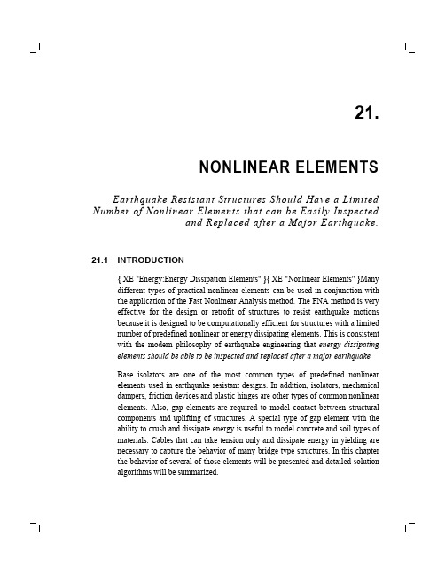
新型装配式剪力墙抗震性能数值模拟与起滑荷载分析

第50 卷第 3 期2023年3 月Vol.50,No.3Mar. 2023湖南大学学报(自然科学版)Journal of Hunan University(Natural Sciences)新型装配式剪力墙抗震性能数值模拟与起滑荷载分析樊禹江1,2†,黄欢欢1,廖凯2,丁佳雄2,葛俊2(1.长安大学建筑学院,陕西西安 710061;2.长安大学建筑工程学院,陕西西安 710061)摘要:为增强装配式剪力墙的耗能能力,提高其施工效益,提出一种具有摩擦抗剪与耗能功能的新型装配式剪力墙结构,并进行了抗震性能试验. 为弥补试件数量不足以及精确确定最优起滑荷载的设计需求,结合新型装配式剪力墙抗震性能试验结果,探讨相应高精度有限元模型建立方法,并进行多参数结构抗震性能影响分析. 最后,基于有限元分析结果和新型装配式剪力墙工作原理,确定最优起滑荷载. 研究结果表明:所提出的新型装配式剪力墙具有良好的滞回耗能能力;螺栓预紧力、钢材摩擦因数、螺栓总距等对结构抗震性能影响显著,应作为相应结构设计的主要参数,竖向荷载、钢板厚度、钢材弹性模量影响较小,可以忽略不计;当起滑荷载设定为墙体屈服荷载时,结构模型耗能达到峰值,同时耗能系数开始明显降低,因而将结构的最优起滑荷载确定为屈服荷载.关键词:装配式结构;抗震性能;有限元模拟;摩擦滑移;屈服荷载中图分类号:TU398. 2 文献标志码:ANumerical Simulation on Seismic Performance of New Prefabricated ShearWalls and Slip Load AnalysisFAN Yujiang1,2†,HUANG Huanhuan1,LIAO Kai2,DING Jiaxiong2,GE Jun2(1. School of Architecture, Chang’an University, Xi’ an 710061, China;2. School of Civil Engineering, Chang’an University, Xi’an 710061, China)Abstract:To improve the energy dissipation capacity and construction benefit of prefabricated shear walls, a new type of prefabricated shear wall structure with the function of friction shear resistance and energy dissipation was proposed, and the seismic performance tests were carried out. To make up for the insufficient quantity of specimens and accurately determine the design requirements of the optimal slip load,based on the seismic performance test results of the proposed structure, this paper discussed the establishment method of the corresponding high-precision finite element model. The multi-parameter analysis of structural seismic performance was carried on. At last, based on the finite element analysis results and the working principle of the new prefabricated shear wall, the optimal slip load was determined. The results show that the proposed new prefabricated shear wall has good hysteretic energy dissipation capacity. Bolt preload, steel friction coefficient and total bolt distance have significant effect on the seismic performance of the structure, and they can be used as the main design parameters of the structure. Vertical load,∗收稿日期:2021-12-20基金项目:国家自然科学基金资助项目(51808046), National Natural Science Foundation of China(51808046)作者简介:樊禹江(1987—),男,陕西西安人,长安大学副教授† 通信联系人,E-mail:*********************文章编号:1674-2974(2023)03-0041-10DOI:10. 16339/j. cnki. hdxbzkb.2023029湖南大学学报(自然科学版)2023 年steel plate thickness and steel elastic modulus have little effects and can be ignored. When the slip load is set as the yield load of the wall, the energy dissipation value of the structure model reaches the peak, and the energy dissipation coefficient begins to decrease significantly. Therefore, the yield load of the wall can be determined as the optimal slip load of the structure.Key words:prefabricated construction;seismic performance;finite element analysis;sliding friction;yield load不同于现浇混凝土结构,装配式建筑具有效率高、污染小、经济效益好等特点,更适应当代社会的需求. 同时,国家对于装配式建筑的大力推广使得国内学者对装配式结构进行了更加深入的研究[1-3]. 其中,装配式连接方法和耗能阻尼装置在装配式结构中的应用已经成为目前的研究热点[4-5]. Henin等[6]提出一种新型钢筋连接套筒灌浆接头,并应用于装配式混凝土构件中. 通过试验对比发现,所设计的钢筋套筒灌浆接头具有良好的力学性能与可靠性.Vaghei 等[7]对所设计的预制混凝土墙体不同竖向连接方法进行了数值模拟,结果表明,预埋钢板螺栓连接试件具有更强的耗能能力. 潘广斌等[8]提出一种采用冷挤压套筒钢筋连接方式的装配式剪力墙构造形式并进行了拟静力试验,结果表明,该连接方法能够有效传递钢筋拉压力,采用该连接形式的装配式剪力墙具有良好的抗震性能. 苗欣蔚等[9]提出一种螺栓连接的全装配式剪力墙水平缝连接方法,开展了5榀试件的单调加载试验,结果表明,该连接方案有效提高了结构变形能力,试件的极限位移角达1/25时仍保持较高的承载力. 孙建等[10]设计出采用螺栓连接的工字形装配式剪力墙并进一步研究了其受力与抗震性能,结果表明,高强螺栓与墙体内嵌边框改善了剪力墙的耗能与延性性能. 徐龙河等[11-13]针对剪力墙受压区易成铰的特点,利用提出的碟簧装置对剪力墙墙脚加以替换,进一步减小了剪力墙的震后损伤,同时实现结构耗能性能的提升. 张偲严等[14]将提出的基于杠杆原理放大变形耗能阻尼器连接于预制装配式剪力墙结构并进行了数值分析,模拟结果表明,相较采用等同现浇的模型,阻尼器连接的结构抗震性能提升显著.本文基于课题组提出的新型装配式剪力墙结构,拟实现结构中小型地震作用下摩擦抗剪抵御水平荷载;在较大地震作用下,上部墙体与水平装置发生相对转动,实现摩擦耗能的功能. 为此,本文结合课题组所作新型装配式剪力墙抗震性能试验结果,探讨了相应结构高精度有限元模型建立方法,并进行多参数结构抗震性能影响分析;最后,基于有限元分析结果,结合新型装配式剪力墙结构工作原理,确定了相应的起滑荷载.1 设计构造新型装配式剪力墙构造设计如图1所示,其中箱形钢、下部槽钢、通长高强螺栓等部件组成水平连接装置[见图1(a)],钢筋混凝土墙体与水平连接装置构成新型装配式剪力墙[见图1(b)]. 为保证墙身与箱形钢的整体连接效果,在箱形钢表面预焊锚固短筋,再与墙体钢筋网架端部焊接连接. 上部整体(墙体+箱形钢)与下部槽钢由钢垫片、通长高强螺栓连接,最后通过施加预紧力实现整体装配. 具体工作原理如下:阶段Ⅰ,当墙体遭受中小型地震时,下部连接装置依靠静摩擦抗剪,抵御水平荷载;阶段Ⅱ,在较大地震作用下,上部整体与下部槽钢板发生相对滑动摩擦,进而消耗地震能量;阶段Ⅲ,上部装置转动至下部槽钢螺孔限位后,水平荷载由墙体和水平连接装置共同承担.2 有限元模拟针对剪力墙的3个工作阶段,课题组设计了相应加载制度并进行了拟静力试验[15].试验加载如图2所示,本文仅针对新型装配式剪力墙工作阶段Ⅰ和阶段Ⅱ的摩擦抗剪、滑移和耗能进行深入研究.因此,基于加载阶段A[见图2(a)]的试验结果,采用ANSYS软件进行分析.具体共建立两个墙体模型与试验结果进行对比验证,编号为XZ-1、XZ-2. 其中,模型XZ-1采用3颗12.9级高强螺栓,螺栓总距为900 mm(各螺栓到装置中心距离为1×0 mm、2×450 mm),螺栓直径为30 mm;模型XZ-2采用5颗10. 9级高强螺栓,螺栓总距为1 500 mm(各螺栓到装42第 3 期樊禹江等:新型装配式剪力墙抗震性能数值模拟与起滑荷载分析置中心距离为1×0 mm 、2×250 mm 、2×500 mm ),螺栓直径为30 mm. 装置中心螺孔均为直径33 mm 的圆形孔,其余位置螺孔依据其与中心螺孔距离,设置宽度为33 mm ,±2 °的圆弧形螺孔滑道. 墙体及水平装置相关建模参数见表1,模型XZ-1几何尺寸及配筋方案(XZ-2与XZ-1配筋相同)见图3.整体采用分离式建模方法,相关材料属性依据试验实测[15]确定. 混凝土本构关系采用《混凝土结构设计规范》(GB 50010—2010)[16]中建议的曲线,钢材本构关系采用有屈服台阶的两线段模型. 为模拟上部墙体与箱形钢之间的固定连接,设置剪力墙下端部钢筋单元均与箱形钢实体单元共用节点的形式. 剪力墙所受竖向荷载根据设计轴压比(见表1)计算确定,水平加载工况与试验加载阶段A 一致,即控制水平位移为15 mm ,以20 kN 为荷载增量对高强螺栓施加110 ~250 kN 共8级预紧力,在每级预紧力工况下,位移往复循环3次. 对于螺栓预紧力采用预紧单元PRETS179进行模拟. 试验中钢板接触面粗糙程度并不均匀,在模拟时不断调整应力较为集中的螺孔局部接触面的摩擦因数,并对比试验数据确保精度要求. 建立的典型试件XZ-1的有限元模型如图4所示.2. 1 模拟结果分析模拟得到典型试件XZ-1的墙体应力云图和螺栓应力云图如图5所示. 可以发现,剪力墙在靠近中(a )水平连接装置(b )新型装配式剪力墙图1 新型装配式剪力墙构造设计Fig. 1 Structural design of new prefabricated shear wall(a )加载制度(b )加载现场图2 试验加载Fig. 2 Test setup 图3 尺寸及配筋详图(单位:mm )Fig. 3 Dimension and steel detailing of specimens (unit :mm )表1 试件设计参数Tab. 1 Main design parameters of the model模型编号XZ-1XZ-2墙体尺寸/mm 1 300×160×1 8201 300×160×1 820摩擦因数0. 190. 19螺栓总距/mm9001 500轴压比0. 250. 2543湖南大学学报(自然科学版)2023 年心螺栓部位应力达到峰值,并沿周围逐渐减弱. 在摩擦滑移时,剪力墙两侧受拉区和受压区区分明显,但应力差距不大,总体处于较低的应力水平,说明剪力墙的损伤较小,这与预期一致.3颗螺栓在初始状态和水平位移加载过程中始终表现为拉-剪受力状态,这是竖向荷载、预紧力和螺孔容差共同作用的结果. 同时,3颗螺栓均满足强度设计要求,其连接性能可靠.模拟得到2组模型在各级预紧力工况下(F N )的荷载-位移(P -∆)曲线结果与试验结果对比如图6(a )(b )(d )(e )所示,可以发现,模拟所得曲线变化 规律与试验结果基本一致,各特征点吻合较好.试 件XZ-1在试验和模拟加载中均未出现开裂,试 件XZ-2试验开裂出现在预紧力为190 kN 、位移为12.55 mm 时,试验开裂荷载为103. 57 kN. 模拟开裂出现在预紧力为170 kN 、位移为15 mm 时,模拟开裂荷载为96. 27 kN ,与试验结果相比,开裂荷载误差为7.05%,表明吻合程度较好. 针对所得滞回曲线进行分析:各阶段曲线均大致呈“方形”,相较传统剪力墙滞回曲线[17],明显多出一水平滞回段,因而滞回面积明显增大,表明新型装配式剪力墙耗能能力高于普通剪力墙. 同时随着螺栓预紧力增大,墙体水平段荷载及曲线滞回面积均呈增大趋势. 结构摩擦抗剪承载力(F )取同一预紧力工况下位移循环3次结果的平均值,将其与试验结果相比,二者误差均小于3%[如图6(c )(f )所示],表明所建新型装配式剪力墙有限元模型能够较为准确地模拟其在水平荷载作用下各阶段的受力特点,可以用于下文理论分析.2. 2 变参模拟基于前述所建新型装配式剪力墙有限元模型,对其进行多参数结构抗震性能分析,所建模型均依次完成15 mm 、20 mm 、25 mm 位移等幅循环加载. 选取的参数为预紧力F N 、摩擦因数μ、螺栓总距∑L 、竖向荷载N 、钢板厚度D 和弹性模量E . 2. 2. 1 螺栓预紧力依据现场试验结果发现,螺栓预紧力对新型装配式剪力墙抗震性能具有较为明显的影响. 模拟时所采用的预紧力模拟工况如表2所示,所得结果如图7所示. 由图7(a )可知,模拟所得滞回曲线饱满,表明结构具有良好的耗能效果,且随着预紧力的增大,滞回面积亦逐渐增大.由图7(b )可知,结构摩擦抗剪承载力与预紧力基本呈正比关系,拟合结果如式(1)所示,在模拟工况范围内摩擦抗剪承载力从61.75 kN 增大到139.29 kN ,增长了125.57%.F =0.693+0.555F N .(1)2. 2. 2 摩擦因数钢材摩擦因数直接影响钢板间摩擦力的大小,试验及模拟结果均表明,结构在转动过程中钢板间动摩擦力与静摩擦力间存在交替转变. 为简化分析,仅考虑钢材动摩擦因数为研究对象,摩擦因数模 拟工况如表3所示,所得结果如图8所示. 结构摩擦抗剪承载力与钢材摩擦因数基本呈正比关系,拟合图5 典型试件XZ-1应力云图Fig. 5 Stress cloud diagram of model XZ-1图4 模型XZ-1有限元模拟Fig. 4 Numerical simulation of model XZ-144第 3 期樊禹江等:新型装配式剪力墙抗震性能数值模拟与起滑荷载分析结果见式(2),在模拟范围内从61.75 kN 增大到128.67 kN ,增大了108.3%.同时,结构滞回面积亦随钢材摩擦因数增大而增大.F =0.944+318.582μ. (2)2. 2. 3 螺栓总距螺栓总距反映结构相对转动时钢板间摩擦路径长度,直接影响结构耗能性能.所建模型的螺栓布置方案如表4所示,螺栓总距依次为900 mm 、1 100 mm 、1 500 mm 、1 900 mm. 模拟结果如图9所示,在结构相对转动过程中墙体所受水平荷载保持稳定,结构摩擦抗剪承载力与螺栓总距基本呈正比关系,拟合结果如式(3)所示,在模拟工况范围内从36.89 kN 增大到77.39 kN ,增长了109. 79%.F =0.158+40.696×10⁻³∑L .(3)2. 2. 4 竖向荷载基于结构轴压比设计分别模拟在竖向荷载为0 kN 、371. 4 kN 、619. 7 kN 、734. 1 kN 时新型装配式剪力墙的滞回性能,模拟工况见表5.模拟结果如图10(a )荷载-位移曲线(b )拟合曲线图7 预紧力的影响Fig. 7 Numerical results of different preloads表2 预紧力工况Tab. 2 Working condition of preloads编号SJ-1SJ-2SJ-3SJ-4F N /kN 110150210250μ0.190.190.190.19∑L /mm 1 5001 5001 5001 500N /kN 619.7619.7619.7619.7D /mm 20202020E /(105MPa )2.102.102.102.10注:表中各模型螺栓总距设置为1 500 mm 时,其布置方案均与模型XZ-2一致.(a )XZ-1模拟数据 (b )XZ-1试验数据 (c )XZ-1拟合曲线(d )XZ-2模拟数据 (e )XZ-2试验数据 (f )XZ-2拟合曲线图6 模拟与试验结果对比Fig. 6 Comparison of simulation and test results45湖南大学学报(自然科学版)2023 年所示,在模拟范围内结构滞回性能无明显变化,结构摩擦抗剪承载力随竖向荷载增加有一定增长,但不明显,在上述模拟过程中,摩擦抗剪承载力从60. 33 kN 增大到62. 01 kN ,增大了2. 78%.2. 2. 5 钢板厚度建立钢板厚度分别为10 mm 、15 mm 、20 mm 、25 mm 的新型装配式剪力墙模型,模拟工况如表6所示,模拟结果如图11所示.可以发现,结构摩擦抗剪承载力随着钢板厚度增大而减小,在模拟范围内从67.67 kN 减小到55.33 kN ,降低了18.23%,曲线滞回面积同样呈减小趋势. 由此表明,钢板厚度的增大对结构抗震性能有一定削弱作用.(a )荷载-位移曲线(b )拟合曲线图9 螺栓总距的影响Fig. 9 Numerical results of different total bolt distances表4 螺栓总距工况Tab. 4 Working condition of total bolt distance编号SJ-9SJ-10SJ-11SJ-12F N /kN 110110110110μ0.190.190.190.19∑L /mm 9001 1001 5001 900N /kN 619.7619.7619.7619.7D /mm 20202020E /(105MPa )2.102.102.102.10注:螺栓总距为900 mm 时,螺栓依次布置为1×0 mm 、2×450 mm ;螺栓总距为1 100 mm 时,螺栓布置依次为1×0 mm 、2×550 mm ;螺栓总距为1 900 mm 时,螺栓依次布置为1×0 mm 、2×400 mm 、2×550 mm.(a )荷载-位移曲线(b )拟合曲线图8 摩擦因数的影响Fig. 8 Numerical results of different friction coefficients表3 摩擦因数工况Tab. 3 Working condition of steel friction coefficient编号SJ-5SJ-6SJ-7SJ-8F N /kN 110110110110μ0. 190. 250. 300. 40∑L /mm 1 5001 5001 5001 500N /kN 619.7619.7619.7619.7D /mm 20202020E /(105MPa )2.102.102.102.10表5 竖向荷载工况Tab. 5 Working condition of vertical loads编号SJ-13SJ-14SJ-15SJ-16F N /kN 110110110110μ0. 190. 190. 190. 19∑L /mm 1 5001 5001 5001 500N /kN 0371. 4619. 7734. 1D /mm 20202020E /(105MPa )2. 102. 102. 102. 1046第 3 期樊禹江等:新型装配式剪力墙抗震性能数值模拟与起滑荷载分析2. 2. 6 钢材弹性模量常用的钢板弹性模量一般在1.95×10⁵~2.10×10⁵MPa 之间,本文分别对钢材弹性模量设置为1.95× 10⁵MPa 、2.00×10⁵MPa 、2. 06×105MPa 、2.10×10⁵MPa的模型进行模拟,具体模拟参数如表7所示,结果如图12所示.结果表明,在模拟范围内,结构滞回性能几乎不变,结构摩擦抗剪承载力变化极小,从60.26 kN 降低到60.16 kN ,变化率仅为0.17%,因此其对结构抗震性能的影响可以忽略.根据上述多参数抗震性能有限元模拟结果可知,结构摩擦抗剪承载力与螺栓预紧力、钢材摩擦因数、螺栓总距均基本呈正比关系,竖向荷载、钢板厚度、钢材弹性模量对结构摩擦抗剪承载力影响较小.该现象符合经典库伦摩擦理论的一般规律,分析认为,墙体工作阶段Ⅱ的水平承载力主要表现为底部钢板间滑动摩擦力产生的转动阻力矩,而摩擦力大小本质上为钢板实际接触面上的法向压力与摩擦因数的乘积. 当其他条件不变仅增大摩擦因数时,摩擦力增大,因而承载力提高;当摩擦因数不变时,接触面法向压力是考虑螺孔周围钢板弹性变形后螺栓预紧力、钢板厚度和钢材弹性模量共同作用的结果;当其他条件不变仅增大竖向荷载时,墙体发生竖向初始滑移,螺杆剪应力增大,在设计强度内对螺栓拉应力无明显影响,因而对钢板接触面法向压力影响较小;当其他条件不变仅增大螺栓总距时,钢板间摩擦表6 钢板厚度工况Tab. 6 Working condition of steel plate thickness编号SJ-17SJ-18SJ-19SJ-20F N /kN 110110110110μ0. 190. 190. 190. 19∑L /mm 1 5001 5001 5001 500N /kN 0000D /mm 10152025E /(105MPa )2. 102. 102. 102. 10表7 钢材弹性模量工况Tab. 7 Working condition of steel elastic modulus编号SJ-21SJ-22SJ-23SJ-24F N /kN 110110110110μ0. 190. 190. 190. 19∑L /mm 1 5001 5001 5001 500N /kN 0000D /mm 20202020E /(105MPa )1. 952. 002. 062. 10(a )荷载-位移曲线(b )拟合曲线图11 钢板厚度的影响Fig. 11 Numerical results of different steel plate thicknesses(a )荷载-位移曲线(b )拟合曲线图10 竖向荷载的影响Fig. 10 Numerical results of different vertical loads47湖南大学学报(自然科学版)2023 年力和墙体转动力臂不变,而钢板间转动阻力臂增大,因而承载力提高.3 起滑荷载的确定针对提出的新型装配式剪力墙,预设最优的起滑荷载可以同时保证结构工作状态的稳定性和预期的抗震性能. 因而有必要研究不同起滑荷载对结构抗震性能的影响规律,具体依次设定墙体开裂荷载、开裂与屈服荷载中点、屈服荷载、峰值荷载为起滑荷载. 结合前述变参分析结果,以及课题组后续针对该新型装配式剪力墙摩擦抗剪实时可变功能的研发,本文仅通过调整螺栓预紧力进行结构起滑荷载设定的分析. 参照前述模型XZ-2进一步建立不同起滑荷载对比分析模型,根据墙体荷载特征点对应的起滑荷载确定螺栓预紧力,剪力墙尺寸、螺栓布置及钢筋配置均与XZ-2相同,钢材间摩擦因数调整为0. 3,其中模型主要设计参数如表8所示.对所建模型进行25 mm 位移等幅加载并循环三次,所得结果如表9,图13、图14所示.由图13可知,随着结构起滑荷载增大,曲线逐渐由“方形”向“梭形”发展,荷载水平段长度减小,荷载上升段与下降段发生明显变化,且该变化趋势在预设起滑荷载越大时越明显. 由此可知,随着预设起滑荷载的增大,墙体在开始转动时弹塑性变形明显(a )荷载-位移曲线(b )拟合曲线图12 钢材弹性模量的影响Fig. 12 Numerical results of different steel elastic modulus(a )QH-1 (b )QH-2(c )QH-3 (d )QH-4图13 不同起滑荷载的荷载-位移曲线Fig. 13 Load-displacement curves of different slip loads(a )总耗能曲线 (b )耗能系数曲线图14 耗能指标变化Fig. 14 Comparison of different energy dissipation indexes表9 耗能指标对比Tab. 9 Comparison of different dissipation indexes编号QH-1QH-2QH-3QH-4总耗能/J 8 302. 714 889. 918 258. 317 636. 3耗能系数3. 633. 272. 712. 29表8 设计参数Tab. 8 Design parameters of the model编号QH-1QH-2QH-3QH-4墙体尺寸/mm 1 300×160×1 8201 300×160×1 8201 300×160×1 8201 300×160×1 820μ0. 30. 30. 30. 3∑L /mm 1 5001 5001 5001 500N /kN 619. 7619. 7619. 7619. 7F N /kN 10821031135048第 3 期樊禹江等:新型装配式剪力墙抗震性能数值模拟与起滑荷载分析增大,结构通过相对转动使摩擦耗能的占比减小. 因而墙体在开始转动前的损伤状态对结构摩擦耗能效果有较大影响,结构起滑荷载不宜过大.根据模拟结果计算得到各模型总耗能值及耗能系数,其随预设起滑荷载的变化规律如图14所示. 结果表明,在墙体达到屈服荷载前,结构总耗能随预设起滑荷载增大而增大,当预设起滑荷载大于墙体屈服荷载后,结构总耗能由于墙体塑性损伤累积而呈下降趋势,结构总耗能峰值主要表现在墙体屈服荷载阶段. 结构耗能系数随预设起滑荷载增大而不断降低,在预设起滑荷载为屈服荷载后开始明显降低,并且在预设起滑荷载为峰值荷载时达到最低.由上述分析可知,针对新型装配式剪力墙起滑荷载的设定需同时考虑结构总耗能值、摩擦抗剪承载力、墙体损伤状态发展、摩擦耗能比等多个因素,综合上述模拟结果以及课题组有关新型装配式剪力墙现场试验数据[18],确定将最优起滑荷载设定为墙体的屈服荷载.4 结论本文提出了一种满足规范各项要求,且能够实现摩擦耗能的新型装配式剪力墙结构,阐述了其工作特征与相关设计参数. 结合试验,针对该新型装配式剪力墙抗震性能进行了多参数分析,进而完成结构最优起滑荷载设定. 主要结论如下:1)基于ANSYS软件,建立了相应的新型装配式剪力墙有限元模型,通过典型试件模拟结果与试验结果的对比分析,验证所建模型能较准确地模拟新型装配式剪力墙在水平荷载作用下各阶段的受力行为,能够应用于结构多参数抗震性能的分析. 2)相较于传统剪力墙结构,新型装配式剪力墙具有更好的抗震性能,尤其是耗能能力明显增强. 3)针对剪力墙的工作阶段Ⅱ进行了多参数抗震性能分析,结果表明,螺栓预紧力、钢材摩擦因数、螺栓总距对结构抗震性能有较显著的影响,摩擦抗剪承载力与三者均基本呈正比关系,应将其作为结构设计的主要参数;竖向荷载、钢板厚度则影响较小,做精细化设计时,可将其设为修正参数;钢材弹性模量影响极小,可忽略不计.4)通过调整螺栓预紧力依次设定墙体开裂荷载、开裂与屈服荷载中点、屈服荷载、峰值荷载为起滑荷载,对所建模型进行抗震性能分析,结果表明:将结构起滑荷载预设为墙体屈服荷载时,结构整体抗震性能良好,结构总耗能达到峰值,之后便伴随着耗能系数的显著降低. 为使结构具有良好的抗震性能与工作性能,应将结构最优起滑荷载预设为墙体屈服荷载.5)研究内容明确了新型装配式剪力墙结构减震机理和一般规律,在此基础上,课题组拟针对高强螺栓连接部位布置智能伸缩材料,通过传感控制实现剪力墙在地震作用下自适应摩擦抗剪功能,完善其在高烈度地区推广应用的技术要求.参考文献[1]VOX G,BLANCO I,SCHETTINI E. Green façades to control wall surface temperature in buildings[J]. Building and Environment,2018,129:154-166.[2]LIU X D,WANG D H,WANG S,et al. Research advances on fabricated shear wall system[J]. IOP Conference Series:MaterialsScience and Engineering,2018,322:042022.[3]孙建,邱洪兴,陆波. 新型全装配式剪力墙结构水平缝节点的机理分析[J]. 湖南大学学报(自然科学版),2014,41(11):15-23.SUN J,QIU H X,LU B. Mechanism analysis on horizontal joints inan innovative precast shear wall system[J]. Journal of HunanUniversity (Natural Sciences),2014,41(11):15-23. (inChinese)[4]赵唯坚,郭婉楠,金峤,等. 预制装配式剪力墙结构竖向连接形式的发展现状[J]. 工业建筑,2014,44(4):115-121.ZHAO W J,GUO W N,JIN Q,et al. State of the art research onconnection type of vertical components for precast concrete shearwall systems[J]. Industrial Construction,2014,44(4):115-121.(in Chinese)[5]XIAO T L,SHENG J C,CHEN Y,et al. Research progress on bolting connection of prefabricated concrete shear wall[J]. IOPConference Series:Materials Science and Engineering,2019,592(1):012013.[6]HENIN E,MORCOUS G. Non-proprietary bar splice sleeve for precast concrete construction[J]. Engineering Structures,2015,83:154-162.[7]VAGHEI R,HEJAZI F,TAHERI H,et al. Development of a new connection for precast concrete walls subjected to cyclic loading[J]. Earthquake Engineering and Engineering Vibration,2017,16(1):97-117.[8]潘广斌,蔡健,杨春,等. 冷挤压套筒连接RC装配式剪力墙抗震性能试验研究[J]. 建筑结构学报,2021,42(5):111-120.PAN G B,CAI J,YANG C,et al. Experimental study on seismic49湖南大学学报(自然科学版)2023 年behavior of precast RC shear walls connected by extruding steelsleeves and rebars[J]. Journal of Building Structures,2021,42(5):111-120. (in Chinese)[9]苗欣蔚,黄炜,胡高兴,等. 水平缝螺栓连接的全装配式复合墙体受力性能试验研究[J]. 湖南大学学报(自然科学版),2021,48(5):19-28.MIAO X W,HUANG W,HU G X,et al. Experimental study onmechanical behavior of fully assembled composite wall with boltedconnection on horizontal joints[J]. Journal of Hunan University (Natural Sciences),2021,48(5):19-28. (in Chinese)[10]孙建,邱洪兴,谭志成,等. 采用螺栓连接的工字形全装配式RC 剪力墙试验研究[J]. 工程力学,2018,35(8):172-183.SUN J,QIU H X,TAN Z C,et al. Experimental study on i-shapedprecast reinforced concrete shear walls using bolted connections[J]. Engineering Mechanics,2018,35(8):172-183. (in Chinese)[11]徐龙河,陈曦,肖水晶. 内置碟簧自复位钢筋混凝土剪力墙拟静力试验及损伤分析[J]. 建筑结构学报,2021,42(7):56-64.XU L H,CHEN X,XIAO S J. Quasi-static test and damageanalysis on self-centering reinforced concrete shear wall with discspring devices[J]. Journal of Building Structures,2021,42(7):56-64. (in Chinese)[12]徐龙河,张焱,肖水晶. 底部铰支自复位钢筋混凝土剪力墙设计与性能研究[J]. 工程力学,2020,37(6):122-130.XU L H,ZHANG Y,XIAO S J. Design and behavior study onbottom hinged self-centering reinforced concrete shear wall[J].Engineering Mechanics,2020,37(6):122-130. (in Chinese)[13]徐龙河,肖水晶. 内置碟簧自复位混凝土剪力墙基于性能的截面设计方法[J]. 工程力学,2020,37(4):70-77.XU L H,XIAO S J. A performance-based section design methodof a self-centering concrete shear wall with disc spring devices[J]. Engineering Mechanics,2020,37(4):70-77. (in Chinese)[14]张偲严,李宏男,李超. 装配式剪力墙高效阻尼器耗能连接的简化模型研究与数值分析[J]. 建筑结构学报,2019,40(10):61-68.ZHANG C Y,LI H N,LI C. Simplified model development andnumerical simulation of a high-efficiency energy-dissipating jointfor prefabricated concrete shear walls[J]. Journal of BuildingStructures,2019,40(10):61-68. (in Chinese)[15]王婧. 新型装配式剪力墙抗震性能试验研究[D]. 西安:长安大学,2021:7-37.WANG J. Experimental study on seismic performance of newprefabricated shear wall[D]. Xi’an:Chang’an University,2021:7-37. (in Chinese)[16]混凝土结构设计规范:GB 50010—2010[S]. 北京:中国建筑工业出版社,2010:209-214.Code for design of concrete structures:GB 50010—2010[S].Beijing:China Architecture & Building Press,2010:209-214.(in Chinese)[17]严涛. 不同连接方式对装配式剪力墙抗震性能的影响[D]. 长沙:湖南大学,2017:26-32.YAN T. The influence of seismic behavior of precast shear wallwith different connection modes[D]. Changsha:Hunan University,2017:26-32. (in Chinese)[18]谭赐. 新型装配式剪力墙摩擦抗剪及设计方法研究[D]. 西安:长安大学,2021:45-63.TAN C. Study on friction for resisting shear and design method ofnew prefabricated shear wall[D]. Xi’an:Chang’an University,2021:45-63. (in Chinese)50。
NONLINEARELEMENTS:非线性元件
21.NONLINEAR ELEMENTS Earthquake Resistant Structures Should Have a Limited Number of Nonlinear Elements that can be Easily Inspectedand Replaced after a Major Earthquake.21.1 INTRODUCTION{ XE "Energy:Energy Dissipation Elements" }{ XE "Nonlinear Elements" }Many different types of practical nonlinear elements can be used in conjunction with the application of the Fast Nonlinear Analysis method. The FNA method is very effective for the design or retrofit of structures to resist earthquake motions because it is designed to be computationally efficient for structures with a limited number of predefined nonlinear or energy dissipating elements. This is consistent with the modern philosophy of earthquake engineering that energy dissipating elements should be able to be inspected and replaced after a major earthquake.Base isolators are one of the most common types of predefined nonlinear elements used in earthquake resistant designs. In addition, isolators, mechanical dampers, friction devices and plastic hinges are other types of common nonlinear elements. Also, gap elements are required to model contact between structural components and uplifting of structures. A special type of gap element with the ability to crush and dissipate energy is useful to model concrete and soil types of materials. Cables that can take tension only and dissipate energy in yielding are necessary to capture the behavior of many bridge type structures. In this chapter the behavior of several of those elements will be presented and detailed solution algorithms will be summarized.。
美国传真图说明

Terminology and Weather SymbolsFRONTSCold front-The leading edge of a relatively colder air mass which separates two air masses in which the gradients of temperature and moisture are maximized. In the northern hemisphere winds ahead of the front will be southwest and shift into the northwest with frontal passage. Frontogenesis-The formation of a front occurs when two adjacent air masses with different densities and temperatures meet and strengthen the discontinuity between the air masses. It occurs most frequently over continental land areas such as over the Eastern US when the air mass moves out over the ocean. It is the opposite of frontolysis.Frontolysis-The weakening or dissipation of a front occurs when two adjacent air masses lose contrasting properties such as the density and temperature. It is the opposite of frontogenesis.Occluded front- The union of two fronts, formed as a cold front overtakes a warm front or quasi-stationary front refers to a cold front occlusion. When a warm front overtakes a cold front or quasi-stationary front the process is termed a warm front occlusion. These processes lead to the dissipation of the front in which there is no gradient in temperature and moisture.Ridge- an elongated area of relatively high pressure that is typically associated with a anti-cyclonic wind shift.Stationary front- A front that has not moved appreciably from its previous analyzed position.Trough- [Trof], an elongated area of relatively low pressure that is typically associated with a cyclonic wind shift.Warm front- The leading edge of a relatively warmer surface air mass which separates two distinctly different air masses. The gradients of temperature and moisture are maximized in the frontal zone. Ahead of a typical warm front in the northern hemisphere, winds are from the southeast and behind the front winds will shift to the southwest.LOW & HIGH PRESSURE SYSTEMS AND MISCELLANEOUS KEY TERMS USEDLow pressure with a number such as 99 means 999 mb and with 03 means 1003 mb. High pressure with a number such as 25 means 1025 mb.Extratropical low- A low pressure center which refers to a migratory frontal cyclone of center and higher latitudes. Tropical cyclones occasionally evolve into extratropical lows losing tropical characteristics and become associated with frontal discontinuity.Low pressure- An area of low pressure identified with counterclockwise circulation in the northern hemisphere and clockwise in the southern hemisphere. Also, defined as a cyclone.High pressure- An area of higher pressure identified with a clockwise circulation in the northern hemisphere and a counterclockwise circulation in the southern hemisphere. Also, defined as an anticyclone.New- The term "NEW" may be used in lieu of a forecast track position of a high or low pressure center when the center is expected to form by a specific time. For example, a surface analysis may depict a 24-hour position of a new low pressure center with an "X" at the 24-hour position followed by the term "NEW", the date and time in UTC which indicates the low is expected to form by 24 hours.Rapidly intensifying- Indicates an expected rapid intensification of a cyclone with surface pressure expected to fall by at least 24 millibar (mb) within 24 hours.Station plotClick for information on coding used with the surface preliminary analysis or for a list of "present weather" symbols.Squall- A sudden wind increase characterized by a duration of minutes and followed by a sudden decrease in winds.Wind speed & DirectionFOGFog-Over the marine environment the term fog refers to visibility greater than or equal to 1/2 NM and less than 3 NM. Fog is the visible aggregate of minute water droplets suspended in the atmosphere near the surface.Dense fog-Over the marine environment the term dense fog refers to visibility less than 1/2 NM. Fog is the visible aggregate of minute water droplets suspended in the atmosphere near the surface.Usually dense fog occurs when air that is lying over a warmer surface such as the Gulf Stream is advected across a colder water surface and the lower layer of the air mass is cooled below its dew point.Sea fog- Common advection fog caused by transport of moist air over a cold body of water.FREEZING SPRAYFreezing spray- Spray in which supercooled water droplets freeze upon contact with exposed objects below the freezing point of water. It usually develops in areas with winds of at least 25 knots.CONVENTIONS USED WITH WARNINGS FOR EXTRATROPICAL SYSTEMS Extratropical SystemsComplex gale/storm-An area in which gale/storm force winds are forecast or are occurring, but in which more than one center is the generating these winds.Developing Gale-Refers to an extratropical low or an area in which gale force winds of 34 knots (39 mph) to47 knots (54 mph) are "expected" by a certain time period. On surface analysis charts, a"DEVELOPING GALE" label indicates gale force winds within the next 24 hours. When the label is used on the 48 hour surface forecast and 96 hour surface forecast charts, gale force winds are expected to develop by 72 hours and 120 hours, respectively.Developing Storm-Refers to an extratropical low or an area in which storm force winds of 48 knots (55 mph) to63 knots (73 mph) are "expected" by a certain time period. On surface analysis charts, a"DEVELOPING STORM" label indicates storm force winds forecast within the next 24 hours.When the label is used on the 48 hour surface and 96 hour surface charts, storm force windsare expected to develop by 72 hours and 120 hours, respectively.Developing Hurricane Force-Refers to an extratropical low or an area in which hurricane force winds of 64 knots (74 mph) or higher are "expected" by a certain time period. On surface analysis charts, a "DEVELOPING HURRICANE FORCE" label indicates hurricane force winds forecast within the next 24 hours. When the label is used on the 48 hour surface and 96 hour surface charts, hurricane force winds are expected to develop by 72 hours and 120 hours, respectively. Gale- Refers to an extratropical low or an area of sustained surface winds (averaged over a ten minute period, momentary gusts may be higher) of 34 knots (39 mph) to 47 knots (54 mph). Storm- Refers to a extratropical low or an area of sustained winds (averaged over a ten minute period, momentary gusts may be higher) of 48 knots (55 mph) to 63 knots (73 mph). Hurricane Force- Refers to a extratropical low or an area of sustained winds (averaged over a ten minute period, momentary gusts may be higher) in excess of 64 knots or higher(74 mph).Small Craft Advisory- Refers to areas within the coastal waters with sustained winds of 18 knots (21 mph) to 33 knots (38 mph).Heavy Freezing Spray-Spray in which supercooled water droplets freeze upon contact with exposed objects below the freezing point of water at the rate of greater than 2 cm/hr. It usually develops in areas with winds of at least 25knots.CONVENTIONS USED WITH WARNINGS FOR TROPICAL SYSTEMSTropical SystemsHurricane- A tropical cyclone with closed contours, a strong and very pronounced circulation, and one minute maximum sustained surface winds 64 knots (74 mph) or greater. A system is called a hurricane over the North Atlantic, Gulf of Mexico, North Pacific E of the dateline, and the South Pacific E of 160E.Intertropical Convergence Zone- (ITCZ) The region where the northeasterly and southeasterly trade winds converge, forming an often continuous band of clouds or thunderstorms near the equator.Post-Tropical- A cyclone that no longer possesses sufficient tropical characteristics to be considered a tropical cyclone. Post-tropical cyclones can continue carrying intense rainfalls and high winds.[Note that former tropical cyclones that have become fully extra-tropical, as well as remnant lows, are two classes of post-tropical cyclones. The term "post-tropical" is predominantly a convenient communications term--to permit the ongoing use of the storm name.]Tropical cyclone- A non-frontal, warm-core, low pressure system of synoptic scale, developing over tropical or subtropical waters with definite organized convection (thunderstorms) and a well defined surface wind circulation.Tropical depression- A tropical cyclone with one or more closed isobars and a one minute max sustained surface wind of less than 34 knots (39 mph).Tropical storm- A tropical cyclone with closed isobars and a one minute max sustained surface wind of 34 knots (39 mph) to 63 knots (73 mph).Typhoon- Same as a hurricane with exception of geographical area. A tropical cyclone with closed contours, a strong and very pronounced circulation, and one minute maximum sustained surface winds of 64 knots (74 mph) or greater. A system is defined as a typhoon over the North Pacific W of the dateline.NOTE: It can be difficult to determine the central pressures of tropical depressions, tropical storms, and hurricanes/typhoons and at times no estimates or measurements is provided by a hurricane or typhoon specialist. An estimate of central pressure may be provided over the Atlantic. Otherwise an XXX is used in place of actual or estimated pressures associated with these systems and an XX is used for forecast central pressure.SEASCombined seas-The combination of both wind waves and swell which is generally referred to as "seas". Primary swell direction- Prevailing direction of swell propagation.Significant wave height- The average height (trough to crest) of the 1/3rd highest waves. An experienced observer will most frequently report the highest 1/3rd of the waves observed.The generation of waves on water results not in a single wave height but in a spectrum of waves distributed from the smallest capillary waves to larger waves. Within this spectrum there is a finite possibility of each of the wave heights to occur with the largest waves being the least likely. The wave height most commonly observed and forecast is the significant wave height. This is defined as the average of the one third highest waves. The random nature of waves implies that individual waves can be substantially higher than the significant wave height. In fact, observations and theory show that the highest individual waves in a typical storm with typical duration to be approximately two times the significant wave height. Somereported rogue waves are well within this factor of two envelope. Waves higher than roughly twice the significant wave height fall into the category of extreme or rogue waves.Swell- Wind waves that have moved out of their fetch or wind generation area. Waves generated by swell exhibit a regular and longer period than wind waves.MISCELLANEOUS TERMINOLOGYCoastal Waters- Includes the area from a line approximating the mean high water along the mainland or island as far out as sixty nautical miles including the bays, harbors and sounds.High Seas- That portion of the Atlantic and Pacific oceans which extends off the Western and Eastern US coasts and extends to 35W in the Atlantic ocean and to 160E in the Pacific Ocean. The area includes both the coastal and offshore waters.Offshore waters- That portion of oceans, gulfs, and seas beyond coastal waters extending to a specified distance from the coastline, to a specified depth contour, or covering an area defined by a specific latitude and longitude points.。
B-Spline插值与回归包的中文名字:B-Spline插值与回归包2.2说明书

Package‘bspline’May26,2023Type PackageTitle B-Spline Interpolation and RegressionVersion2.2Author Serguei Sokol<**********************>Maintainer Serguei Sokol<**********************>Description Build and use B-splines for interpolation and regression.In case of regression,equality constraints as well as monotonicityand/or positivity of B-spline weights can be imposed.Moreover,knot positions(not only spline weights)can be part ofoptimized parameters too.For this end,'bspline'is able to calculateJacobian of basis vectors as function of knot er is provided withfunctions calculating spline values at arbitrary points.Thesefunctions can be differentiated and integrated to obtain B-splines calculatingderivatives/integrals at any point.B-splines of this package cansimultaneously operate on a series of curves sharing the same set ofknots.'bspline'is written with concern about computingperformance that's why the basis and Jacobian calculation is implemented in C++.The rest is implemented in R but without notable impact on computing speed. URL https:///MathsCell/bsplineBugReports https:///MathsCell/bspline/issuesLicense GPL-2Encoding UTF-8Imports Rcpp(>=1.0.7),nlsic(>=1.0.2),arrApplyLinkingTo Rcpp,RcppArmadilloRoxygenNote7.2.3Suggests RUnitCopyright INRAE/INSA/CNRSNeedsCompilation yesRepository CRANDate/Publication2023-05-2615:00:02UTC12bcurve R topics documented:bcurve (2)bsc (3)bsp (4)bspline (5)bsppar (6)dbsp (6)diffn (7)dmat (7)ibsp (8)iknots (9)ipk (9)jacw (10)par2bsp (10)parr (11)smbsp (11)Index15 bcurve nD B-curve governed by(x,y,...)control points.DescriptionnD B-curve governed by(x,y,...)control points.Usagebcurve(xy,n=3)Argumentsxy Real matrix of(x,y,...)coordinates,one control point per row.n Integer scalar,polynomial order of B-spline(3by default)DetailsThe curve will pass by thefirst and the last points in’xy’.The tangents at thefirst and last points will coincide with thefirst and last segments of control points.Example of signature is inspired from this blog.ValueFunction of one argument calculating B-curve.The argument is supposed to be in[0,1]interval.bsc3 Examples#simulate doctor s signature;)set.seed(71);xy=matrix(rnorm(16),ncol=2)tp=seq(0,1,len=301)doc_signtr=bcurve(xy)plot(doc_signtr(tp),t="l",xaxt= n ,yaxt= n ,ann=FALSE,frame.plot=FALSE, xlim=range(xy[,1]),ylim=range(xy[,2]))#see where control points aretext(xy,labels=seq(nrow(xy)),col=rgb(0,0,0,0.25))#join them by segmentslines(bcurve(xy,n=1)(tp),col=rgb(0,0,1,0.25))#randomly curved wire in3D space##Not run:if(requireNamespace("rgl",quite=TRUE)){xyz=matrix(rnorm(24),ncol=3)tp=seq(0,1,len=201)curv3d=bcurve(xyz)rgl::plot3d(curv3d(tp),t="l",decorate=FALSE)}##End(Not run)bsc Basis matrix and knot Jacobian for B-spline of order0(step function)and higherDescriptionThis function is analogous but not equivalent to splines:bs()and splines2::bSpline().It is also several times faster.Usagebsc(x,xk,n=3L,cjac=FALSE)Argumentsx Numeric vector,abscissa pointsxk Numeric vector,knotsn Integer scalar,polynomial order(3by default)cjac Logical scalar,if TRUE makes to calculate Jacobian of basis vectors as function of knot positions(FALSE by default)4bsp DetailsFor n==0,step function is defined as constant on each interval[xk[i];xk[i+1][,i.e.closed on theleft and open on the right except for the last interval which is closed on the right too.The Jacobianfor step function is considered0in every x point even if in points where x=xk,the derivative is notdefined.For n==1,Jacobian is discontinuous in such points so for these points we take the derivative fromthe right.ValueNumeric matrix(for cjac=FALSE),each column correspond to a B-spline calculated on x;or List(for cjac=TRUE)with componentsmat basis matrix of dimension nx x nw,where nx is the length of x and nw=nk-n-1is the number of basis vectorsjac array of dimension nx x(n+2)x nw where n+2is the number of support knots for each basis vectorSee Alsosplines::bs(),splines2::bSpline()Examplesx=seq(0,5,length.out=101)#cubic basis matrixn=3m=bsc(x,xk=c(rep(0,n+1),1:4,rep(5,n+1)),n=n)matplot(x,m,t="l")stopifnot(all.equal.numeric(c(m),c(splines::bs(x,knots=1:4,degree=n,intercept=TRUE)))) bsp Calculate B-spline values from their coefficients qw and knots xkDescriptionCalculate B-spline values from their coefficients qw and knots xkUsagebsp(x,xk,qw,n=3L)bspline5Argumentsx Numeric vector,abscissa points at which B-splines should be calculated.They are supposed to be non decreasing.xk Numeric vector,knots of the B-splines.They are supposed to be non decreasing.qw Numeric vector or matrix,coefficients of B-splines.NROW(qw)must be equal to length(xk)-n-1where n is the next parametern Integer scalar,polynomial order of B-splines,by default cubic splines are calcu-lated.DetailsThis function does nothing else than calculate a dot-product between a B-spline basis matrix cal-culated by bsc()and coefficients qw.If qw is a matrix,each column corresponds to a separate set of coefficients.For x values falling outside of xk range,the B-splines values are set to0.To get a function calculating spline values at arbitrary points from xk and qw,cf.par2bsp().ValueNumeric matrix(column number depends on qw dimensions),B-spline values on x.See Alsobsc,par2bspbspline bspline:build and use B-splines for interpolation and regression.DescriptionBuild and use B-splines for interpolation and regression.In case of regression,equality constraints as well as monotonicity requirement can be imposed.Moreover,knot positions(not only spline coefficients)can be part of optimized parameters er is provided with functions calculating spline values at arbitrary points.This functions can be differentiated to obtain B-splines calculating derivatives at any point.B-splines of this package can simultaneously operate on a series of curves sharing the same set of knots.’bspline’is written with concern about computing performance that’s why the basis calculation is implemented in C++.The rest is implemented in R but without notable impact on computing speed.bspline functions•bsc:basis matrix(implemented in C++)•bsp:values of B-spline from its coefficients•dbsp:derivative of B-spline•par2bsp:build B-spline function from parameters•bsppar:retrieve B-spline parameters from its function6dbsp•smbsp:build smoothing B-spline•fitsmbsp:build smoothing B-spline with optimized knot positions•diffn:finite differencesbsppar Retrieve parameters of B-splinesDescriptionRetrieve parameters of B-splinesUsagebsppar(f)Argumentsf Function,B-splines such that returned by par3bsp(),smbsp(),...ValueList having components:n-polynomial order,qw-coefficients,xk-knotsdbsp Derivative of B-splineDescriptionDerivative of B-splineUsagedbsp(f,nderiv=1L,same_xk=FALSE)Argumentsf Function,B-spline such as returned by smbsp()or par2bsp()nderiv Integer scalar>=0,order of derivative to calculate(1by default)same_xk Logical scalar,if TRUE,indicates to calculate derivative on the same knot grid as original function.In this case,coefficient number will be incremented by2.Otherwise,extreme knots are removed on each side of the grid and coefficientnumber is maintained(FALSE by default).ValueFunction calculating requested derivativediffn7Examplesx=seq(0.,1.,length.out=11L)y=sin(2*pi*x)f=smbsp(x,y,nki=2L)d_f=dbsp(f)xf=seq(0.,1.,length.out=101)#fine grid for plottingplot(xf,d_f(xf))#derivative estimated by B-splineslines(xf,2.*pi*cos(2*pi*xf),col="blue")#true derivativexk=bsppar(d_f)$xkpoints(xk,d_f(xk),pch="x",col="red")#knot positionsdiffn Finite differencesDescriptionCalculate dy/dx where x,y arefirst and the rest of columns in the entry matrix’m’Usagediffn(m,ndiff=1L)Argumentsm2-or more-column numeric matrixndiff Integer scalar,order offinite difference(1by default)ValueNumeric matrix,first column is midpoints of x,the second and following are dy/dxdmat Differentiation matrixDescriptionCalculate matrix for obtaining coefficients offirst-derivative B-spline.They can be calculated as dqw=Md%*%qw.Here,dqw are coefficients of thefirst derivative,Md is the matrix returned by this function,and qw are the coefficients of differentiated B-spline.Usagedmat(nqw=NULL,xk=NULL,n=NULL,f=NULL,same_xk=FALSE)8ibspArgumentsnqw Integer scalar,row number of qw matrix(i.e.degree of freedom of a B-spline) xk Numeric vector,knot positionsn Integer scalar,B-spline polynomial orderf Function from which previous parameters can be retrieved.If both f and anyof previous parameters are given then explicitly set parameters take precedenceover those retrieved from f.same_xk Logical scalar,the same meaning as in dbspValueNumeric matrix of size nqw-1x nqwibsp Indefinite integral of B-splineDescriptionIndefinite integral of B-splineUsageibsp(f,const=0,nint=1L)Argumentsf Function,B-spline such as returned by smbsp()or par2bsp()const Numeric scalar or vector of length ncol(qw)where qw is weight matrix of f.Defines starting value of weights for indefinite integral(0by default).nint Integer scalar>=0,defines how many times to take integral(1by default) DetailsIf f is B-spline,then following identity is held:Dbsp(ibsp(f))is identical to f.Generally,it does not work in the other sens:ibsp(Dbsp(f))is not f but not very far.If we can get an appropriate constant C=f(min(x))then we can assert that ibsp(Dbsp(f),const=C)is the same as f.ValueFunction calculating requested integraliknots9 iknots Estimate internal knot positions equalizing jumps in n-th derivativeDescriptionNormalized total variation of n-thfinite differences is calculated for each column in y then averaged.These averaged values arefitted by a linear spline tofind knot positions that equalize the jumps of n-th derivative.NB.This function is used internally in(fit)smbsp()and a priori has no interest to be called directly by user.Usageiknots(x,y,nki=1L,n=3L)Argumentsx Numeric vectory Numeric vector or matrixnki Integer scalar,number of internal knots to estimate(1by default)n Integer scalar,polynomial order of B-spline(3by default)ValueNumeric vector,estimated knot positionsipk Intervals of points in knot intervalsDescriptionFindfirst and last+1indexes iip s.t.x[iip]belongs to interval starting at xk[iik]Usageipk(x,xk)Argumentsx Numeric vector,abscissa points(must be non decreasing)xk Numeric vector,knots(must be non decreasing)ValueInteger matrix of size(2x length(xk)-1).Indexes are0-based10par2bsp jacw Knot Jacobian of B-spline with weightsDescriptionKnot Jacobian of B-spline with weightsUsagejacw(jac,qws)Argumentsjac Numeric array,such as returned by bsc(...,cjac=TRUE)qws Numeric matrix,each column is a set of weights forming a B-spline.If qws is a vector,it is coerced to1-column matrix.ValueNumeric array of size nx x ncol(qw)x nk,where nx=dim(jac)[1]and nk is the number of knots dim(jac)[3]+n+1(n being polynomial order).par2bsp Convert parameters to B-spline functionDescriptionConvert parameters to B-spline functionUsagepar2bsp(n,qw,xk,covqw=NULL,sdy=NULL,sdqw=NULL)Argumentsn Integer scalar,polynomial order of B-splinesqw Numeric vector or matrix,coefficients of B-splines,one set per column in case of matrixxk Numeric vector,knotscovqw Numeric Matrix,covariance matrix of qw(can be estimated in smbsp).sdy Numeric vector,SD of each y column(can be estimated in smbsp).sdqw Numeric Matrix,SD of qw thus having the same dimension as qw(can be esti-mated in smbsp).parr11 ValueFunction,calculating B-splines at arbitrary points and having interface f(x,select)where x is a vector of abscissa points.Parameter select is passed to qw[,select,drop=FALSE]and can be missing.This function will return a matrix of size length(x)x ncol(qw)if select is missing.Elsewhere,a number of column will depend on select parameter.Column names in the result matrix will be inherited from qw.parr Polynomial formulation of B-splineDescriptionPolynomial formulation of B-splineUsageparr(xk,n=3L)Argumentsxk Numeric vector,knotsn Integer scalar,polynomial order(3by default)ValueNumeric3D array,thefirst index runs through n+1polynomial coefficients;the second–through n+1supporting intervals;and the last one through nk-n-1B-splines(here nk=length(xk)).Knot interval of length0will have corresponding coefficients set to0.smbsp Smoothing B-spline of order n>=0DescriptionOptimize smoothing B-spline coefficients(smbsp)and knot positions(fitsmbsp)such that residual squared sum is minimized for all y columns.Usagesmbsp(x,y,n=3L,xki=NULL,nki=1L,lieq=NULL,monotone=0,positive=0,mat=NULL,estSD=FALSE,tol=1e-10)fitsmbsp(x,y,n=3L,xki=NULL,nki=1L,lieq=NULL,monotone=0,positive=0,control=list(),estSD=FALSE,tol=1e-10)Argumentsx Numeric vector,abscissa pointsy Numeric vector or matrix or data.frame,ordinate values to be smoothed(one set per column in case of matrix or data.frame)n Integer scalar,polynomial order of B-splines(3by default)xki Numeric vector,strictly internal B-spline knots,i.e.lying strictly inside of x bounds.If NULL(by default),they are estimated with the help of iknots().This vector is used as initial approximation during optimization process.Mustbe non decreasing if not NULL.nki Integer scalar,internal knot number(1by default).When nki==0,it corresponds to polynomial regression.If xki is not NULL,this parameter is ignored.lieq List,equality constraints to respect by the smoothing spline,one list item per y column.By default(NULL),no constraint is imposed.Constraints are given asa2-column matrix(xe,ye)where for each xe,an ye value is imposed.If a listitem is NULL,no constraint is imposed on corresponding y column.monotone Numeric scalar or vector,if monotone>0,resulting B-spline weights must be increasing;if monotone<0,B-spline weights must be decreasing;if monotone==0(default),no constraint on monotonicity is imposed.If’monotone’is avector it must be of length ncol(y),in which case each component indicatesthe constraint for corresponding column of y.positive Numeric scalar,if positive>0,resulting B-spline weights must be>=0;if positive<0,B-spline weights must be decreasing;if positive==0(default),no constraint on positivity is imposed.If’positive’is a vector it must be oflength ncol(y),in which case each component indicates the constraint for cor-responding column of y.mat Numeric matrix of basis vectors,if NULL it is recalculated by bsc().If pro-vided,it is the responsibility of the user to ensure that this matrix be adequate toxki vector.estSD Logical scalar,if TRUE,indicates to calculate:SD of each y column,covariance matrix and SD of spline coefficients.All these values can be retrieved withbsppar()call(FALSE by default).These estimations are made under assumptionthat all y points have uncorrelated noise.Optional constraints are not taken intoaccount of SD.tol Numerical scalar,relative tolerance for small singular values that should be con-sidered as0if s[i]<=tol*s[1].This parameter is ignored if estSD=FALSE(1.e-10by default).control List,passed through to nlsic()callDetailsIf constraints are set,we use nlsic::lsie_ln()to solve a least squares problem with equality constraints in least norm sens for each y column.Otherwise,nlsic::ls_ln_svd()is used for the whole y matrix.The solution of least squares problem is a vector of B-splines coefficients qw,one vector per y column.These vectors are used to define B-spline function which is returned as the result.NB.When nki>=length(x)-n-1(be it from direct setting or calculated from length(xki)),it corresponds to spline interpolation,i.e.the resulting spline will pass exactly by(x,y)points(well, up to numerical precision).Border and external knots arefixed,only strictly internal knots can move during optimization.The optimization process is constrained to respect a minimal distance between knots as well as to bound them to x range.This is done to avoid knots getting unsorted during iterations and/or going outside of a meaningful range.ValueFunction,smoothing B-splines respecting optional constraints(generated by par2bsp()).See Alsobsppar for retrieving parameters of B-spline functions;par2bsp for generating B-spline function;iknots for estimation of knot positionsExamplesx=seq(0,1,length.out=11)y=sin(pi*x)+rnorm(x,sd=0.1)#constraint B-spline to be0at the interval endsfsm=smbsp(x,y,nki=1,lieq=list(rbind(c(0,0),c(1,0))))#check parameters of found B-splinesbsppar(fsm)plot(x,y)#original"measurements"#fine grained xxfine=seq(0,1,length.out=101)lines(xfine,fsm(xfine))#fitted B-splineslines(xfine,sin(pi*xfine),col="blue")#original function #visualize knot positionsxk=bsppar(fsm)$xkpoints(xk,fsm(xk),pch="x",col="red")#fit broken line with linear B-splinesx1=seq(0,1,length.out=11)x2=seq(1,3,length.out=21)x3=seq(3,4,length.out=11)y1=x1+rnorm(x1,sd=0.1)y2=-2+3*x2+rnorm(x2,sd=0.1)y3=4+x3+rnorm(x3,sd=0.1)x=c(x1,x2,x3)y=c(y1,y2,y3)plot(x,y)f=fitsmbsp(x,y,n=1,nki=2)lines(x,f(x))Indexbcurve,2bsc,3bsp,4bspline,5bsppar,6dbsp,6,8diffn,7dmat,7fitsmbsp(smbsp),11ibsp,8iknots,9ipk,9jacw,10par2bsp,10parr,11smbsp,10,1115。
一种高效的阻尼器优化设计方法

Vol37 No5Sept 2020第37卷第5期2020年9月建筑科学与工程学报Journal of Architecture and Civil Engineering引用本文:李钢,翟子杰,余丁浩•一种高效的阻尼器优化设计方法"#建筑科学与工程学报,2020,37(5):5-61.LI Gang,ZHAI Zi-jie,YU Ding-hao. An Efficient Optimal Design Method for Dampers"# Journal of Architecture and Civil Engineering, 2020,37(5):51-61.DOI : 10. 19815/j. jace. 2019. 05106一种高效的阻尼器优化设计方法李钢,翟子杰,余丁浩(大连理工大学海岸和近海工程国家重点实验室,辽宁大连116024)摘要:以隔离非线性方法为基袖,并对基于种群的可行性遗传算法进行改进,提出了 一种高效的阻尼器优化设计方法。
首先基于隔离非线性方法基本思想,分别推导了附加位移型和速度型阻尼器消能减震结构的隔离非线性控制方程;随后,采用基于种群可行性约束优化遗传算法对其中的初始种群生成方法及交叉、变异、选择算子进行改进,7提高算法在可行域边界附近的搜索能力;最后, 通过对某钢结构增设金属阻尼器进行工程加固,验证了该方法的准确性和高效性。
结果表明:新方法拓展了隔离非线性方法的应用范围,提高了遗传算法在可行域边界附近的搜索能力和设计中的 计算效率,是一种高效的阻尼器优化设计方法。
关键词:消能减震结构;隔离非线性方法;阻尼器;优化设计;遗传算法 中图分类号:TU352. 1文献标志码:A文章编号:1673-2049(2020)05-0051-11An Efficient Optimal Design Method for DampersLI Gang , ZHAI Zi-jie , YU Ding-hao(State Key Laboratory of Costal and O f shore Engineering !Dalian UniversityofTechnology !Dalian116024!Liaoning !China )Abstract : Based on inelasticity-separated finite element method (IS-FEM) and the improvement ofgenetic algorithm based on population feasibility, an efficient optimal design method for dampess was proposed Firstly !based on the basicidea ofIS-FEM !theisolation nonlinear control equations of structure equipped with displacement-based dampess and velocity-based dampesswere derived respectively Then !the constrained optimization genetic algorithm based on population feasibility was adopted and the population initialization method !crossover !mutationand selection operators were modified to improve the searching ability near feasible regionboundary Fina l y !asteelstructureretrofitprojectwith meta l icyieldingdamperswastakenasexampletoverifytheaccuracyande f iciencyoftheproposedmethod Theresultsshowthatthe new methodexpandstheapplicationrangeofIS-FEM !improvesthesearch ability of genetic algorithm near the boundary of feasible region, and improves the calculation efficiency in design .Theproposedmethodisane f icientoptimizationdesign methodofdamperKey words : energy dissipation structure ; inelasticity-separated finite element method ; damper ;optimal design ; genetic algorithm收稿日期:2019-10-11基金项目:国家重点研发计划项目(2018YFD1100404);国家自然科学基金项目$1878112);大连市高层次人才创新支持计划项目(2017RD04)作者简介:李 钢(1979-),男,辽宁葫芦岛人,教授,博士研究生导师,工学博士,E-mail :gli@dlut. edu. cn 。
ANSYS-CFX

ANSYS CFX-Pre User Guide1、CFX-Pre Basics:1、Starting CFX-Pre:File >> New Case;General:通用CFX-Pre界面,用于所有类型CFD模拟;Turbomachinery:涡轮机械CFD模拟;Quick Setup:CFX-Pre简化,仅用于单计算域(single-domain)、单相(single-phase)问题模拟;不支持:多相(multiphase)、燃烧(combustion)、辐射(radiation)、高等湍流模型(advanced turbulence models)CFD模拟。
Library Template:模板库提供特定物理模拟模板;2、CFX-Pre W orkspace:Outline 结构:(1)Mesh:网格操作如:导入(import)、变换(transformation)、渲染(render)、可视化(show、hide)(2)Simulation:AnalysisAnalysis Type:稳态(steady)、瞬态(transient)分析,Domain:流体(fluid)、多孔介质(porous)、固体(solid)计算域,区域、类型、属性设置;Domain Interfaces:计算域、网格连接界面;Global Initialization:全局计算域初始化,单一计算域初始化于Domain中设置;Solver:求解单位(Solution Units)、求解控制(Solver Control)、输出控制(Output Control);Coordinate Frame:默认笛卡尔坐标系,可创建新坐标系统;Materials、Reactions:材料、化学反应;Expressions、Functions、V ariables:表达式、自定义函数、变量、及子程序;(3)Simulation Control:分析求解控制、及求解结构序列(Configuration)设置;(4)Case Options:显示、标示设置;3、CFS-Pre 文件类型:(1)Case File(.cfx):CFX-Pre数据文件,包括模拟物理学定义、计算区域设置、网格信息;(2)Mesh File:网格文件;(3)CFX-Solver Input Files(.def,.mdef):CFX-Solver输入文件,单一结构输入文件(.def);多结构输入文件(.mdef),需补充构造序列(Configuration Definition)定义文件(.cfg);(4)CFS-Solver Results File(.res,.mres,.trn,.bak):结果文件(.res单一结构,.mres多结构),多结构模拟.mres文件,同时可生成单一.res结果文件;中间结果文件(.trn瞬态结果文件,.bak备份文件),Output Control >> Trn Results、Backup设置;(5)CFX-Solver Error Results File(.err):CFX-Solver求解失败错误信息文件;(6)Session File(.pre):CFX-Pre录制CCL操作命令;(7)CCL File(CFX Command Language,.ccl):CFX-Pre保存CCL 命令状态文件,较Session File,仅对当前CCL命令操作状态保存。
FLUENT13培训教材08物理模型-ANSYS公司

Slug Flow
Bubbly, Droplet, or Particle-Laden Flow
Stratified / FreePneumatic Transport, Surface Flow Hydrotransport, or Slurry Flow
气/固 固
液/固 固
Sedimentation
有不同化学属性的材料但属于同一种物理相如液液多相流体系统分为一种主流体相和多种次流体相可以有多种次流体相代表不同尺寸的颗粒primaryphasesecondaryphasesperaglobalcompanyperachina多相流体系气泡流连续液体中存在离散的气泡如气体吸收器蒸发设备鼓泡设备液滴流连续气体中的离散液滴如喷雾器燃烧器柱塞流连续液体中的大尺度气泡分层自由表面流不相溶的流体被清晰的界面分开如自由表面流颗粒流连续气体中的离散固体颗粒如旋风分离器空气净化器吸尘器流化床流化床反应器泥浆流液体中的固体颗粒固体悬浮沉积液力输运pneumatictransporthydrotransportslurryflowfluidizedbedsedimentationstratifiedfreesurfaceflowslugflowbubblydropletparticleladenflowperaglobalcompanyperachinafluent中的多相流模型fluent包括四种不同的多相流模型
1.1 mm
0.2 mm
欧拉模型的例子 – 三维气泡床
z = 20 cm
z = 15 cm
z = 10 cm
z = 5 cm
Isosurface of Gas Volume Fraction = 0.175
Liquid Velocity Vectors
PDE_lecture_3

Leonard Euler 1707-1783
FTCS-Method is basically useless!
• Why? • Algorithm is numerical unstable.
12
What is numerical stability?
Say we have to add 100 numbers of array a[i] using a computer with only 2 significant digits.
Forward in time
Centered in space
9
Euler method, FTCS
Forward in Time Centered in Space
10
Euler method, FTCS
Forward in Time Centered in Space
Show: demo_advection.pro
John von Neumann 1903-1957
14
Von Neumann stability analysis
Ansatz: Wave number k and amplification factor:
A numerical scheme is unstable if:
15
Von Neumann stability analysis
29
Phase Errors
• We rewrite the stability condition:
• A wave packet is a superposition of many waves with different wave numbers k. • Numerical scheme multiplies modes with different phase factors. • => Numerical dispersion. • The method is exact if CFL is fulfilled exactly: (Helps here but not in inhomogenous media.)
- 1、下载文档前请自行甄别文档内容的完整性,平台不提供额外的编辑、内容补充、找答案等附加服务。
- 2、"仅部分预览"的文档,不可在线预览部分如存在完整性等问题,可反馈申请退款(可完整预览的文档不适用该条件!)。
- 3、如文档侵犯您的权益,请联系客服反馈,我们会尽快为您处理(人工客服工作时间:9:00-18:30)。
a r X i v :0711.4685v 1 [g r -q c ] 29 N o v 2007A new dissipation term for finite-difference simulations in RelativityDaniela Alic,Carles Bona and Carles Bona-Casas Departament de Fisica,Universitat de les Illes Balears Institute for Applied Computation with Community Code (IAC 3).Abstract.We present a new numerical dissipation algorithm,which can be efficiently used in combination with centered finite-difference methods.We start from a formulation of centered finite-volume methods for Numerical Relativity,in which third-order space accuracy can be obtained by employing just piecewise-linear reconstruction.We obtain a simplified version of the algorithm,which can be viewed as a centered finite-difference method plus some ’adaptive dissipation’.The performance of this algorithm is confirmed by numerical results obtained from 3D black hole simulations.1.Introduction In a recent paper (Alic et al 2007),we presented a centered finite-volume (CFV)method for black-hole simulations in numerical relativity.This method is a variant of the well known local-Lax-Friedrichs approach (LLF),which is currently being used in computational fluid dynamics (including magneto-hydrodynamics).For a specific choice of the parameters,this method can be written as a piecewise-fourth-order finite-difference (FD)algorithm plus a piecewise-third-order accurate artificial dissipation,with automatically tuned local coefficient.The piecewise prefix comes from the slope limiters that are incorporated in order to deal with shocks or other discontinuities.Current black hole simulations in Numerical Relativity use instead centered FD algorithms combined with a numerical dissipation term of the Kreiss-Oliger type (Gustafson et al 1995).This combination can be interpreted as a single numerical scheme with built-in dissipation,which can be tuned by a single parameter.In most numerical relativity simulations,where only smooth profiles are dealt with,this hasshown to be an efficient computational approach.In some black hole simulations,however,the required amount of dissipation varies from the inner to the outer regions,so this approach is lacking some flexibility.Our main point is that,as far as the slope limiters are not required,the FV algorithm which we developed can be expressed also as a fourth-order centered FD algorithms combined with a local dissipation term which is automatically adapted to the requirements of the either interior or exterior black hole regions.2.The Centered Finite-Volume Method in a Flux-Splitting Approach We consider the Einstein field equations written as a system of balance laws∂t u +∂k F k (u )=S (u ),(1)where the Flux terms F and the Source terms S depend algebraically on the array of dynamicalfields u.We will considerfirst the one-dimensional case.In a regular finite difference grid,we choose the elementary cell to be the interval(x i−1/2,x i+1/2) centered in the grid point x i.The resulting discrete scheme is given byu n+1 i =u n i−∆t2σ+i,F−R=F−i+1−12(F+L+F−R).(5)3.Third-order-accurate Dissipation FormulaLet us write the prescription for the slopes of theflux components generically as σ+i=aσL i+(1−a)σR i,σ−i=bσL i+(1−b)σR i,(6) where a and b are slope coefficients,and we have noted for shortσL i=F±i−F±i−1,σR i=F±i+1−F±i.(7) We determine the specific values of the slope coefficients which allow third order accuracy,by inserting the slope formulae in the CFV paring thefinal algorithm with the standard fourth orderfinite difference method,one obtains the values a=1/3,b=2/3for the slope coefficients.If no slope limiters are implemented, the derivative of theflux can be expressed in closed form asD x(F i)=112∆x[λi+2u i+2−4λi+1u i+1+6λi u i−4λi−1u i−1+λi−2u i−2].(9) We test the stability and convergence of the resulting algorithm in the Gauge Wave Test(Fig.1),one of the standard tests for Numerical Relativity(Alcubierre et0.9 0.95 1 1.05 1.1-0.4-0.2 00.2 0.4g x x x 2 2.533.54-0.4-0.2 0 0.2 0.4o r d e r x Figure 1.3D Gauge-Wave test simulations.The profiles in the left panel areplots of the metric component g xx for three resolutions (∆x =0.02,0.01,0.005)after 100crossing times;the last two almost coincide.The right panel shows thelocal convergence rate,calculated by comparing the two higher resolutions withthe exact solution,confirming third-order convergence.al 2004).The plots show that the resulting amount of dissipation is actually very small and confirm third-order convergence.Note,however,that in this case all the local λcoefficients are equal to one,so the new dissipation term coincides with the Kreiss-Oliger one for a specific value of its global coefficient.4.The 3D Black HoleThe dissipation algorithm presented above can be easily extended to the 3D case:Dis (F x i,j,k )=1Let us consider initial data taken from a Schwarzschild black holeMds2=−α2dt2+(1+。