R语言时间序列作业
R语言常用上机命令分功能整理——时间序列分析为主

R语言常用上机命令分功能整理——时间序列分析为主第一讲应用实例•R的基本界面是一个交互式命令窗口,命令提示符是一个大于号,命令的结果马上显示在命令下面。
•S命令主要有两种形式:表达式或赋值运算(用’<-’或者’=’表示)。
在命令提示符后键入一个表达式表示计算此表达式并显示结果。
赋值运算把赋值号右边的值计算出来赋给左边的变量。
•可以用向上光标键来找回以前运行的命令再次运行或修改后再运行。
•S是区分大小写的,所以x和X是不同的名字。
我们用一些例子来看R软件的特点。
假设我们已经进入了R的交互式窗口。
如果没有打开的图形窗口,在R中,用:> x11() 可以打开一个作图窗口。
然后,输入以下语句:x1 = 0:100x2 = x1*2*pi/100y = sin(x2)plot(x2,y,type="l")这些语句可以绘制正弦曲线图。
其中,“=”是赋值运算符。
0:100表示一个从0到100 的等差数列向量。
第二个语句可以看出,我们可以对向量直接进行四则运算,计算得到的x2 是向量x1的所有元素乘以常数2*pi/100的结果。
从第三个语句可看到函数可以以向量为输入,并可以输出一个向量,结果向量y的每一个分量是自变量x2的每一个分量的正弦函数值。
plot(x2,y, type="l",main="画图练习",sub="好好练", xlab="x轴",ylab='y轴')有关作图命令plot的详细介绍可以在R中输入help(plot)数学函数abs,sqrt:绝对值,平方根 log, log10, log2 , exp:对数与指数函数 sin,cos,tan,asin,acos,atan,atan2:三角函数 sinh,cosh,tanh,asinh,acosh,atanh:双曲函数简单统计量sum, mean, var, sd, min, max, range, median, IQR(四分位间距)等为统计量,sort,order,rank与排序有关,其它还有ave,fivenum,mad,quantile,stem等。
时间序列分析R语言代码

时间序列分析R语言代码时间序列分解分析的R语言操作如下:选取R语言自带的数据包UKgas,即1960-1986每月英国天然气消耗的数据,并将其赋值于n:n<-UKgassummary()函数提供了最小值、最大值、四分位数和数值型变量的均值: summary(n)画出UKgas的时序图:plot(n)时间序列分解分析方法一:基础包stats的decompose函数调用基础包stats:library("stats")利用基础包stats的decompose函数对时间序列进行分解分析,命名为fit1。
该函数基于移动平均方法,multiplicative表示使用乘法模型:fit1=decompose(n, type = c("multiplicative"))展示decompose函数的分解结果:fit1绘制方法一,即利用decompose函数分解的分解图:plot(fit1)`时间序列分解分析方法二:基础包stats的stl函数stl函数stl(x,s.window,s.degree=0,t.window = NULL, t.degree = 1, robust = FALSE,na.action = na.fail)x----待分解的变量s.window----提取季节性时的loess算法时间窗口宽度,可设为periodic,或者设为奇数并不能低于7s.degree -----提取季节性时局部拟合多项式的阶数,须为0或1 t.window----提取长期趋势性时的loess算法时间窗口宽度,缺省为NULL,或者奇数t.degree-----提取长期趋势性时的局部拟合多项式的阶数,须为0或1robust -----在loess过程中是否使用鲁棒拟合利用基础包stats的stl函数对时间序列进行分解分析,命名为fit2:fit2<-stl(n,s.window="periodic",s.degree = 0, t.window = NULL, t.degree = 1,robust= FALSE,na.action = na.fail)展示stl函数的分解结果:fit2绘制方法二的分解图: plot(fit2)。
时间序列分析-基于R(第五章作业)
时间序列分析第五章作业T1(p164第1题):程序:rm(list=ls())# 清空工作环境P5T1data=read.table("C:\\Users\\DMXTC\\Documents\\SJXLZY_data\\E5_1.txt ",header=T)r5_1<-as.matrix(P5T1data$货运量)d5_1<-as.vector(t(r5_1))T5_1<-ts(d5_1,start=1949)# 绘制时序图par(mfrow=c(1,1))plot(T5_1,type = "o",col="blue",pch=13,main="表5-2时序图")diff_T5_1<-diff(T5_1)#1阶差分plot(diff_T5_1,type = "o",col="blue",pch=13,main="一阶差分后时序图")# ADF检验library(aTSA)adf.test(diff_T5_1)# 纯随机性检验for (k in 1:2)print(Box.test(diff_T5_1,lag=6*k))# 绘制自相关图和偏自相关图par(mfrow=c(1,2))acf(diff_T5_1)pacf(diff_T5_1)# x<-window(T5_1,start=1949,end = 1998)# test<-window(T5_1,start=1999)library(forecast)fit1<-Arima(T5_1,order=c(1,1,0),include.drift=T)fit1tsdiag(fit1)fore1<-forecast::forecast(fit1,h=5)fore1par(mfrow=c(1,1))plot(fore1,lty=2)lines(fore1$fitted,col=4)分析:首先我们绘制时序图如下:时序图显示该序列具有显著线性递增趋势,这是典型的非平稳序列特征,对该序列进行1阶差分,差分后时序图如下:差分后序列基本围绕在0值附近波动,已经没有明显的趋势特征,为进一步确定差分后序列的平稳性,对差分后的序列进行ADF检验,其检验结果显示如下:> adf.test(diff_T5_1)Augmented Dickey-Fuller Testalternative: stationaryType 1: no drift no trendlag ADF p.value[1,] 0 -3.24 0.0100[2,] 1 -2.78 0.0100[3,] 2 -1.95 0.0498Type 2: with drift no trendlag ADF p.value[1,] 0 -4.13 0.0100[2,] 1 -3.84 0.0100[3,] 2 -2.97 0.0462Type 3: with drift and trendlag ADF p.value[1,] 0 -4.69 0.0100[2,] 1 -4.46 0.0100[3,] 2 -3.63 0.0381----Note: in fact, p.value = 0.01 means p.value <= 0.01检验结果显示,该序列所有ADF检验统计量的P值均小于显著性水平(α=0.05),所以可以确定1阶差分后系列实现了平稳。
时间序列分析R语言程序

#例2.1绘制196 ------- 1999年中国年纱产量序列时序图(数据见附录1.2)Data1.2=read.csv("C:\\Users\\Administrator\\Desktop\\ 附录1.2.csv",header=T)#如果有标题,用T;没有标题用Fplot(Data1.2,type='o')#例2.1续tdat1.2=Data1.2[,2]a1.2=acf(tdat1.2)#例2.2绘制1962年1月至1975年12月平均每头奶牛产奶量序列时序图(数据见附录1.3)Data1.3=read.csv("C:\\Users\\Administrator\\Desktop\\ 附录 1.3.csv”,header=F)tdat1.3=as.vector(t(as.matrix(Data1.3)))[1:168]# 矩阵转置转向量plot(tdat1.3,type=T)#例2.2续acf(tdat1.3) #把字去掉pacf(tdat1.3)#例2.3绘制1949——1998年北京市每年最高气温序列时序图Data1.4=read.csv("C:\\Users\\Administrator\\Desktop\\ 附录 1.4.csv”,header=T)plot(Data1.4,type='o')##不会定义坐标轴#例2.3续tdat1.4=Data1.4[,2]a1.4=acf(tdat1.4)#例2.3续Box.test(tdat1.4,type="Ljung-Box”,lag=6)Box.test(tdat1.4,type="Ljung-Box”,lag=12)#例2.4随机产生1000个服从标准正态分布的白噪声序列观察值,并绘制时序图Data2.4=rnorm(1000,0,1)Data2.4plot(Data2.4,type=T)#例2.4续a2.4=acf(Data2.4)#例2.4续Box.test(Data2.4,type="Ljung-Box”,lag=6)Box.test(Data2.4,type="Ljung-Box”,lag=12)#例2.5对195 ——1998年北京市城乡居民定期储蓄所占比例序列的平稳性与纯随机性进行检验Data1.5=read.csv("C:\\Users\\Administrator\\Desktop\\ 附录 1.5.csv”,header=T)plot(Data1.5,type='o',xlim=c(1950,2010),ylim=c(60,100) )tdat1.5=Data1.5[,2]a1.5=acf(tdat1.5)#白噪声检验Box.test(tdat1.5,type="Ljung-Box”,lag=6)Box.test(tdat1.5,type="Ljung-Box”,lag=12)#例2.5续选择合适的ARMA模型拟合序列acf(tdat1.5)pacf(tdat1.5)#根据自相关系数图和偏自相关系数图可以判断为AR(1)模型#例2.5续P81 口径的求法在文档上#P83arima(tdat1.5,order=c(1,0,0),method="ML")# 极大似然估计ar1=arima(tdat1.5,order=c(1,0,0),method="ML") summary(ar1)ev=ar1$residualsacf(ev)pacf(ev)#参数的显著性检验t1=0.6914/0.0989p1=pt(t1,df=48,lower.tail=F)*2#ar1的显著性检验t2=81.5509/ 1.7453p2=pt(t2,df=48,lower.tail=F)*2#残差白噪声检验Box.test(ev,type="Ljung-Box”,lag=6,fitdf=1)Box.test(ev,type="Ljung-Box”,lag=12,fitdf=1)#例2.5续P94预测及置信区间predict(arima(tdat1.5,order=c(1,0,0)),n.ahead=5)tdat1.5.fore=predict(arima(tdat1.5,order=c(1,0,0)),n.ahea d=5)U=tdat1.5.fore$pred+1.96*tdat1.5.fore$seL=tdat1.5.fore$pred-1.96*tdat1.5.fore$seplot(c(tdat1.5,tdat1.5.fore$pred),type="l”,col=1:2)lines(U,co l=”blue”,lty=”dashed”)lines(L,col=”blue”,lty=”dashed”)#例3.1.1例3.5 例3.5续#方法一plot.ts(arima.sim(n=100,list(ar=0.8)))#方法二x0=runif(1)x=rep(0,1500)x[1]=0.8*x0+rnorm(1) for(i in 2:length(x)) {x[i]=0.8*x[i-1]+rnorm(1)} plot(x[1:100],type=T) acf(x)pacf(x)##拟合图没有画出来x[1]=x1x[2 ]=-x1-0.5*x0+rnorm(1)for(i in 3:length(x)){x[i]=-x[i-1]-0.5*x[i-2]+rnorm(1)} plot(x[1:100],type=T)acf(x)pacf(x)#例3.1.2x0=runif(1)x=rep(0,1500)x[1]=-1.1*x0+rnorm(1) for(i in 2:length(x)) #均值和方差smu=mean(x) svar=var(x){x[i]=-1.1*x[i-1]+rnorm(1)} plot(x[1:100],type=T) acf(x) pacf(x) #例3.2求平稳AR (1)模型的方差例3.3 mu=0 mvar=1/(1-0.8A2) #书上51 页#总体均值方差#例3.1.3方法一plot.ts(arima.sim(n=100,list(ar=c(1,-0.5)))) #方法二x0=runif(1)x1=runif(1)x=rep(0,1500)x[1]=x1x[2]=x1-0.5*x0+rnorm(1)for(i in 3:length(x)){x[i]=x[i-1]-0.5*x[i-2]+rnorm(1)}plot(x[1:100],type=T)acf(x)pacf(x) cat("population mean and var are”,c(mu,mvar),"\n")#样本均值方差cat("sample mean and var are”,c(mu,mvar),"\n")#例题3.4svar=(1+0.5)/((1-0.5)*(1-1-0.5)*(1+1-0.5))#例题3.6 MA模型自相关系数图截尾和偏自相关系数图拖尾#3.6.1法:x=arima.sim(n=1000,list(ma=-2))plot.ts(x,type='l')acf(x)#例3.1.4x0=runif(1)x1=runif(1)x=rep(0,1500)x[1]=x1x[2]=x1+0.5*x0+rnorm(1)for(i in 3:length(x)){x[i]=x[i-1]+0.5*x[i-2]+rnorm(1)} plot(x[1:100],type=T)acf(x)pacf(x) pacf(x)法二x=rep(0:1000)for(i in 1:1000){x[i]=rnorm[i]-2*rnorm[i-1]} plot(x,type=T)acf(x)pacf(x)#3.6.2法一:又一个式子x0=runif(1)x1=runif(1)x=rep(0,1500) x=arima.sim(n=1000,list(ma=-0.5)) plot.ts(x,type='l')acf(x)pacf(x)法二x=rep(0:1000)for(i in 1:1000){x[i]=rnorm[i]-0.5*rnorm[i-1]}plot(x,type='l')acf(x)pacf(x)##错误于rnorm[i]:类别为'closure'的对象不可以取子集#3.6.3法^:x=arima.sim(n=1000,list(ma=c(-4/5,16/25)))plot.ts(x,type=T)acf(x)pacf(x)法二:x=rep(0:1000)for(i in 1:1000) {x[i]=rnorm[i]-4/5*rnorm[i-1]+16/25*rnorm[i-2]} plot(x,type='l')acf(x)pacf(x)##错误于x[i] = rnorm[i] - 4/5 * rnorm[i - 1] + 16/25 * rnorm[i - 2] :##更换参数长度为零#例3.6续根据书上64页来判断#例3.7拟合ARMA ( 1,1)模型,x(t)-0.5x(t-1)=u(t)-0.8*(u-1),并直观观察该模型自相关系数和偏自相关系数的拖尾性。
用R语言做时间序列分析

用R语言做时间序列分析时间序列(time series )是一系列有序的数据。
通常是等时间间隔的采样数据。
如果不是等间隔,则一般会标注每个数据点的时间刻度。
下面以time series 普遍使用的数据airline passenger 为例。
这是^一年的每月乘客数量,单位是千人次。
Time如果想尝试其他的数据集,可以访问这里:https:///data/list/?q=provider:tsdl可以很明显的看出,airli ne passe nger 的数据是很有规律的。
time series data mining 主要包括decompose (分析数据的各个成分,例如趋势,周期性),prediction (预测未来的值),classificatio n (对有序数据序列的feature 提取与分类),clusteri ng (相似数列聚类)等。
这篇文章主要讨论prediction (forecast,预测)问题。
即已知历史的数据,如何准确预测未来的数据。
先从简单的方法说起。
给定一个时间序列,要预测下一个的值是多少,最简单的思路是什么呢?(1)m ean (平均值):未来值是历史值的平均。
(2)exponential smoothing (指数衰减):当去平均值得时候,每个历史点的权值可以不一样。
最自然的就是越近的点赋予越大的权重。
= aX± + ct^X2 + a3X3+ …或者,更方便的写法,用变量头上加个尖角表示估计值X t+1 = aX t+ (1 - a)X t(3) sn aive :假设已知数据的周期,那么就用前一个周期对应的时刻作为下一个周期对应时刻的预测值(4)d rift :飘移,即用最后一个点的值加上数据的平均趋势tX t+h|t =禺+占2心-斗-丄= x t +占(罠-如Tt = •介绍完最简单的算法,下面开始介绍两个time series 里面最火的两个强大的算法:Holt-Winters 和ARIMA 。
用R语言实现奶牛月产奶量的时间序列分析

⽤R语⾔实现奶⽜⽉产奶量的时间序列分析奶⽜⽉产奶量的时间序列分析本⽂应⽤R软件对奶⽜⽉产奶量建⽴时间序列模型并进⾏预测。
⽂章主要从以下⼏个⽅⾯进⾏:1.描述性统计2.模型识别3.参数估计4.模型诊断5.预测6.其他建模⽅法及效果对⽐7.结论最终通过多⽅⾯对⽐,我们选择了ARIMA(0,1,1)×(0,1,1)12模型⽤于以后数据的预测。
⼀、描述性统计1.1数据的选取本⽂引⽤的是Data Market中的时间序列数据“Monthly milk production: pounds per cow. Jan 62 –Dec 75”,包括从1962年1⽉到1975年12⽉共168个⽉度数据,单位为pounds/month。
数据如下:从中我们将62-74年,共156条数据作为训练集,75年的12个⽉数据作为测试集,⽤于最后评价模型预测效果的参考。
1.2数据的描述性统计变量统计表1-1数据类型最⼩值下四分数中位数均值上四分数最⼤值数值型数据553.0 677.8 761.0 754.7 824.5 969.0时间序列的分布图和时间序列的分解如下:时间序列分解图1-1由图可以看出,时间序列含有明显的季节性和上升趋势,且没有波动集群现象,可以考虑季节模型,最常⽤的是ARIMA模型。
1.3乘法季节模型乘法季节模型是随机季节模型与 ARIMA 模型的结合。
统计学上纯 RIMA (p,d, q )模型记作:ΦΘ。
其中 t 代表时间,Xt 表⽰响应序列,B是后移算⼦, R=1-B,p、 d、 q 分别表⽰⾃回归阶数、差分阶数和移动平均阶数;Φ(B)表⽰⾃回归算⼦;Θ(B)表⽰滑动平均算⼦。
⼀个阶数为(P,d, q )×(P, D, Q ) s 的乘积季节模型可表为:ΦΘ代表独⽴⼲扰项或随机误差项, s 的值是⼀个季节循环中观测的个数,atΦ表⽰同⼀周期内不同周期点的相关关系,则描述了不同周期中对应时点上的相关关系,⼆者结合起来便同时刻画了 2 个因数的作⽤。
课后习题答案-时间序列分析及应用(R语言原书第2版)
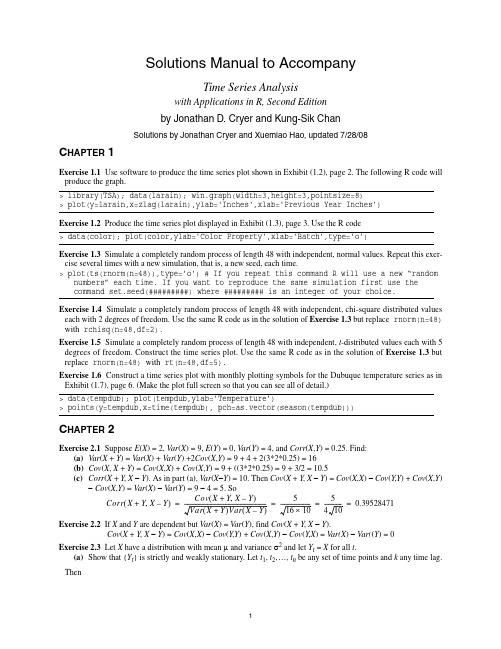
stationary.
(b) Find the autocovariance function for {Yt}. Cov(Yt,Yt − k) = Cov(X,X) = σ2 for all t and k, free of t (and k). (c) Sketch a “typical” time plot of Yt. The plot will be a horizontal “line” (really a discrete-time horizontal line)
relation functions are the same for θ = 3 and θ = 1/3. For simplicity, suppose that the process mean is known
to be zero and the variance of Yt is known to be 1. You observe the series {Yt} for t = 1, 2,..., n and suppose that you can produce good estimates of the autocorrelations ρk. Do you think that you could determine which value of θ is correct (3 or 1/3) based on the estimate of ρk? Why or why not?
如何使用R语言进行时间序列分析与预测

如何使用R语言进行时间序列分析与预测标题:使用R语言进行时间序列分析与预测导言:时间序列分析是一种用于研究随时间变化的数据模式和趋势的方法。
它在许多领域中都有广泛的应用,包括经济学、金融学、气象学等。
R语言是一种功能强大的统计分析软件,它提供了许多用于时间序列分析和预测的函数和包。
本文将介绍如何使用R语言进行时间序列分析和预测的步骤和方法。
一、准备数据1. 收集时间序列数据:首先需要收集相关的时间序列数据,例如每天的销售量、股票价格等。
这些数据可以通过调查、采样或从公开数据源中获取。
2. 数据清洗:对收集到的数据进行清洗,包括去除异常值、缺失值和重复值等。
确保数据的完整性和准确性。
3. 建立时间索引:将数据转换为时间序列对象,并建立时间索引。
R语言中常用的时间序列对象包括ts、xts和zoo等。
二、时间序列分析1. 可视化分析:使用R语言中的绘图函数,如plot()和ggplot2包,将时间序列数据可视化。
可以观察数据的趋势、季节性和周期性。
2. 平稳性检验:检验时间序列数据是否平稳,即均值、方差和自协方差不随时间变化。
常用的平稳性检验方法有ADF检验和KPSS检验。
3. 建立模型:根据时间序列数据的特点选择合适的模型。
常用的时间序列模型包括ARIMA模型、指数平滑模型和ARCH/GARCH模型等。
4. 模型识别:对建立的模型进行参数估计,并进行模型识别。
使用R语言中的函数,如auto.arima()和ets(),自动选择最佳的模型。
5. 模型诊断:对建立的模型进行诊断,检验模型的拟合优度。
常用的模型诊断方法有残差分析、Ljung-Box检验和AIC准则等。
三、时间序列预测1. 预测模型:基于建立的时间序列模型,使用R语言中的forecast包,预测未来一段时间内的数值。
可以使用函数,如forecast()和predict(),进行预测。
2. 模型评估:对时间序列预测结果进行评估。
使用预测准确度指标,如均方根误差(RMSE)和平均绝对百分误差(MAPE),评估预测模型的准确性。
- 1、下载文档前请自行甄别文档内容的完整性,平台不提供额外的编辑、内容补充、找答案等附加服务。
- 2、"仅部分预览"的文档,不可在线预览部分如存在完整性等问题,可反馈申请退款(可完整预览的文档不适用该条件!)。
- 3、如文档侵犯您的权益,请联系客服反馈,我们会尽快为您处理(人工客服工作时间:9:00-18:30)。
points(y=rstudent(hours.lm),x=as.vector(time(hours)),pch=as.vector(season(hours)))
3.10(a)data(hours);hours.lm=lm(hours~time(hours)+I(time(hours)^2));summary(hours.lm)
用最小二乘法拟合二次趋势,结果显示如下:
Call:
lm(formula = hours ~ time(hours) + I(time(hours)^2))
Residual standard error: 0.423 on 57 degrees of freedom
Multiple R-squared: 0.5921, Adjusted R-squared: 0.5778
F-statistic: 41.37 on 2 and 57 DF, p-value: 7.97e-12
正态性检验(Shapiro-Wilk检验)本质是:计算残差与相应的正态分位数之间的相关系数。相关性越小,就越有理由否定正态性。
Shapiro-Wilk normality test
data: rstudent(hours.lm)
W = 0.99385, p-value = 0.9909
根据上面的检验结果,我们不能拒绝模型的随机项是正态分布的假设。
Residuals:
Min 1Q Median 3Q Max
-1.00603 -0.25431 -0.02267 0.22884 0.98358
Coefficients:
Estimate Std. Error t value Pr(>|t|)
(Intercept) -5.122e+05 1.155e+05 -4.433 4.28e-05 ***
time(hours) 5.159e+02 1.164e+02 4.431 4.31e-05 ***
I(time(hours)^2) -1.299e-01 2.933e-02 -4.428 4.35e-05 ***
---
Signif. codes: 0‘***’0.001‘**’0.01‘*’0.05‘.’0.1‘’1
5.7(a) A:AR(2)φ1=0.9φ2=0.09
B:IMA(1,1)Θ1=0.1
(b)一个是固定的一个是不固定的。
5.11(a)data(nebago);win.graph(width=6.5,height=3,pointsize=8)
plot(winnebago,type='o',ylab='Winnebago Monthly Sales')
标准残差的时间序列,应用月度绘图标志。(为了更容易识别季节性)
带季节性图标的的残差-时间图
(c)runs(rstudent(hours.lm))
对标准差进行游程检验
$pvalue
[1] 0.00012
$observed.runs
[1] 16
$expected.runs
[1] 30.96667
$n1
[1] 31
(QQ图)
正态性可以通过正态得分或者分位数-分位数(QQ)图来检验。此处的直线型图形支持了该模型中随机项是正态分布的假设。
hist(rstudent(hours.lm),xlab='Standardized Residuals')
标准残差的直方图(季节均值模型的标准残差直方图)
shapiro.test(rstudent(hours.lm))
win.graph(width=3,height=3,pointsize=8)
plot(x=diff(log(winnebago))[-1],y=percentage[-1],ylab='Percentage Change',xlab='Difference of Logs')
cor(diff(log(winnebago))[-1],percentage[-1])
$n2
[1] 29
$k
[1] 0
结果解释:P值为0.00012,表明非随机性是合理的。
(d)acf(rstudent(hours.lm))
标准残差的样本自相关函数
季节均值模型残差的样本自相关系数
(e)qqnorm(rstudent(hours.lm));qqline(rstudent(hours.lm))
第四章平稳时间序列模型
4.4
第五章非平稳时间序列模型
5.1(a) ARMA (2,1) p=2,q=1,参数值φ和θ
φ1=1φ2=-0.25Θ1=0.1
(b) IMA(2,0) p=2,d=1,q=0,参数值φ和θ
(c) ARMA(2,2) p=2,q=2,参数值φ和θ
φ1=0.5φ2=-0.5Θ1=0.5Θ2=-0.25
时间序列图
表明公司的休闲车的销量在逐渐增加。
(b)plot(log(winnebago),type='o',ylab='Log(Monthly Sales)')
取对数之后的时间序列图
仍然呈现增加的趋势,但是比没有取对数之前增加的缓慢一些。
(c)percentage=na.omit((winnebago-zlag(winnebago))/zlag(winnebago))
[1] 0.9646886
2016年第二学期时间序列分析及应用R语言课后作业
第三章趋势
3.4(a)data(hours);plot(hours,ylab='Monthly Hours',type='o')
画出时间序列图
(b)data(hours);plot(hours,ylab='Monthly Hours',type='l')
type='o'表示每个数据点都叠加在曲线上;type='b'表示在曲线上叠加数据点,但是该数据点附近是断开的;type='l'表示只显示各数据点之间的连接线段;type='p'只想显示数据点。
points(y=hours,x=time(hours),pch=as.vector(season(hours)))