95个EXCEL常用技巧(快捷键+常用函数)速查版
Excel操作技巧速查手册个让你轻松操作的快捷键
Excel操作技巧速查手册个让你轻松操作的快捷键Excel操作技巧速查手册:个人让你轻松操作的快捷键Excel是一款广泛应用于各行各业的强大电子表格软件。
无论你是初学者还是经验丰富的用户,学会使用一些Excel操作技巧和快捷键,可以帮助你提高工作效率和数据处理能力。
本速查手册将为你介绍一些常用的Excel操作技巧及其对应的快捷键,帮助你轻松操作Excel。
一、常用的快捷键1. 新建工作簿:Ctrl+N2. 打开工作簿:Ctrl+O3. 保存工作簿:Ctrl+S4. 另存为:F125. 关闭工作簿:Ctrl+W6. 退出Excel:Alt+F47. 撤销:Ctrl+Z8. 重做:Ctrl+Y9. 剪切:Ctrl+X10. 复制:Ctrl+C11. 粘贴:Ctrl+V12. 选择全部:Ctrl+A13. 查找:Ctrl+F14. 替换:Ctrl+H15. 删除单元格内容:Delete16. 删除整行或整列:Ctrl+-17. 插入单元格:Ctrl+Shift+=18. 插入整行或整列:Ctrl+Shift++(加号)19. 移动到下一个工作表:Ctrl+PgDn20. 移动到上一个工作表:Ctrl+PgUp二、编辑和格式化技巧1. 快速编辑单元格:双击单元格2. 填充单元格序列:选中需要填充的单元格,将鼠标移到单元格右下角,出现黑色十字,向下拖动鼠标即可自动填充序列3. 设置文本自动换行:选中需要自动换行的单元格,右键点击单元格,选择“格式单元格”,进入对话框,选择“对齐”选项卡中的“自动换行”4. 合并单元格:选中需要合并的单元格,右键点击单元格,选择“格式单元格”,进入对话框,选择“对齐”选项卡中的“合并单元格”5. 设置数字格式:选中需要设置格式的单元格,右键点击单元格,选择“格式单元格”,进入对话框,选择“数字”选项卡,选择相应的数字格式6. 设置边框:选中需要设置边框的单元格或区域,右键点击单元格,选择“格式单元格”,进入对话框,选择“边框”选项卡,选择相应的边框样式7. 设置自动筛选:选中包含数据的区域,点击“数据”选项卡上的“排序和筛选”,选择“筛选”三、公式和函数技巧1. 输入公式:在单元格中输入“=”后,输入相应的公式2. 快速求和:选中一列或一行数据,查看状态栏上的求和值3. 平均值:选中一列或一行数据,查看状态栏上的平均值4. 最大值和最小值:选中一列或一行数据,查看状态栏上的最大值和最小值5. 查找特定数值:使用“查找与选择”功能,通过指定条件查找特定数值6. 合并单元格求和:使用“合并单元格”时,使用SUM函数求和合并区域的数值7. 计算百分比:使用百分比格式,或用数值除以总数后乘以100得到百分比值四、数据操作技巧1. 排序:选中需要排序的区域,点击“数据”选项卡上的“排序”2. 筛选:选中需要筛选的区域,点击“数据”选项卡上的“排序和筛选”,选择“筛选”3. 数据透视表:选中需要创建透视表的区域,点击“插入”选项卡上的“透视表”4. 数据验证:选中需要设置验证的区域,右键点击单元格,选择“数据验证”,进入对话框,设置验证条件5. 文本拆分:选中需要拆分的文本列,点击“数据”选项卡上的“文本到列”6. 去重:选中需要去重的区域,点击“数据”选项卡上的“删除重复项”7. 填充日期和时间:输入开始日期或时间,选中需要填充的单元格区域,点击右键选择“填充”,选择“序列”,选择需要的序列类型,点击确定填充五、其它常用技巧1. 快速切换工作表:Ctrl+PageUp和Ctrl+PageDown2. 分屏显示:点击“视图”选项卡上的“新建窗口”,然后在“视图”选项卡上点击“拆分”3. 设置打印区域:选中需要打印的区域,点击“页面布局”选项卡上的“打印区域”,选择“设置打印区域”4. 创建图表:选中需要创建图表的数据区域,点击“插入”选项卡上的“图表”,选择所需的图表类型5. 设置打印标题:选中需要设置的打印行或列,点击“页面布局”选项卡上的“打印标题”6. 设置批注:选中需要添加批注的单元格,右键点击单元格,选择“插入批注”7. 使用快速分析工具:选中需要分析的数据区域,点击“数据”选项卡上的“快速分析”六、总结通过掌握这些Excel操作技巧和快捷键,你可以在使用Excel时更加高效和便捷。
Excel函数、公式、快捷方式操作大全(动画版)
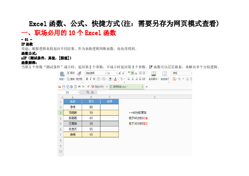
Excel函数、公式、快捷方式(注:需要另存为网页模式查看) 一、职场必用的10个Excel函数- 01 -IF函数用途:根据逻辑真假返回不同结果。
作为表格逻辑判断函数,处处用得到。
函数公式:=IF(测试条件,真值,[假值])函数解释:当第1个参数“测试条件”成立时,返回第2个参数,不成立时返回第3个参数。
IF函数可以层层嵌套,来解决多个分枝逻辑。
- 02 -SUMIF和SUMIFS函数用途:对一个数据表按设定条件进行数据求和。
- SUMIF函数 -函数公式:=SUMIF(区域,条件,[求和区域])函数解释:参数1:区域,为条件判断的单元格区域;参数2:条件,可以是数字、表达式、文本;参数3:[求和区域],实际求和的数值区域,如省略则参数1“区域”作为求和区域。
- SUMIFS函数 -函数公式:=SUMIFS(求和区域,区域1,条件1,[区域2],[条件2],……)函数解释:第1个参数是固定求和区域。
区别SUMIF函数的判断一个条件,SUMIFS函数后面可以增加多个区域的多个条件判断。
- 03 -VLOOKUP函数用途:最常用的查找函数,用于在某区域内查找关键字返回后面指定列对应的值。
函数公式:=VLOOKUP(查找值,数据表,列序数,[匹配条件])函数解释:相当于=VLOOKUP(找什么,在哪找,第几列,精确找还是大概找一找)最后一个参数[匹配条件]为0时执行精确查找,为1(或缺省)时模糊查找,模糊查找时如果找不到则返回小于第1个参数“查找值”的最大值。
- 04 -MID函数用途:截取一个字符串中的部分字符。
有的字符串中部分字符有特殊意义,可以将其截取出来,或对截取的字符做二次运算得到我们想要的结果。
函数公式:=MID(字符串,开始位置,字符个数)函数解释:将参数1的字符串,从参数2表示的位置开始,截取参数3表示的长度,作为函数返回的结果。
- 05 -DATEDIF函数用途:计算日期差,有多种比较方式,可以计算相差年数、月数、天数,还可以计算每年或每月固定日期间的相差天数、以及任意日期间的计算等,灵活多样。
常用Excel函数和快捷键说明
常用Excel函数说明1、自动编号函数:=MAX($A$1:A1)+1含义:如果A1编号为1,那么A2=MAX($A$1:A1)+1。
假设A1为1,那么在A2中输入“=MAX($A$1:A1)+1”,回车。
然后用填充柄将公式复制到其他单元格即可。
2、统计某一区域某一数据出现的次数函数:=COUNTIF(K4:K60,”新开”)含义:统计K4到K60单元格中“新开”出现的次数。
假设在K61中输入“新开”,在K62中输入“=COUNTIF(K4:K60,”新开”)”后回车,即可统计出K4至K60单元格中“新开”出现的次数。
3、避免输入相同的数据函数:=COUNTIF(A:A,A2)=1含义:在选定的单元格区域中保证输入的数据的唯一性。
假设在A列中避免输入重复的姓名,先选中相应的单元格区域,如A2至A500,依次选中“数据-有效性-设置”,在“允许”下拉栏中选“自定义”,在“公式”栏中输入“=COUNTIF(A:A,A2)=1”。
单击“确定”完成。
4、在单元格中快速输入当前日期函数:=today()含义:快速输入当前日期,并可随系统时间自动更新。
方法:在选中单元格中输入“=today()”回车,即可输入当前日期。
5、在单元格中快速输入当前日期及时间函数:=now()含义:快速输入当前日期及时间,并可随系统时间自动更新。
方法:在选中单元格中输入“=now()”回车,即可输入当前日期及时间。
6、缩减小数点后的位数函数:=TRUNC(A1,1)含义:将两位小数点变为一位小数点。
方法:例如,A1的数值为“36.99”,需要在B1中显示A1数值小数点后的一位,则在B1中直接输入函数表达式“=TRUNC(A1,1)”,而后将在B1中显示“36.9”。
7、将数据合二为一函数:=CONCATENATE(A1,B1)含义:将Excel中的两列数据合并至一列中。
方法:如果要将Excel中的两列数据合并至一列中,可以使用文本合并函数。
excel快捷键函数公式表
excel快捷键函数公式表Excel是一款非常强大的电子表格软件,它提供了许多功能,如数据统计、分析、展示等。
为了更高效地使用Excel,了解其快捷键、函数和公式是非常重要的。
本文将为您介绍一些常用的Excel快捷键、函数和公式,以帮助您更好地完成工作。
一、快捷键1. 常用快捷键Ctrl+C:复制Ctrl+V:粘贴Ctrl+A:全选Ctrl+Z:撤销操作Ctrl+N:新建工作簿Ctrl+S:保存工作簿2. 单元格操作快捷键Delete:删除单元格内容Backspace:删除上一单元格内容Alt+Enter:显示单元格内容格式Alt+Shift+方向键:快速调整单元格格式3. 窗口操作快捷键F5:定位对话框F8:逐个选择单元格Ctrl+Tab:快速切换工作表Alt+PageDown/PageUp:切换窗口二、常用函数1. SUM函数:用于求和。
2. AVERAGE函数:用于求平均值。
3. MAX函数:用于求最大值。
4. MIN函数:用于求最小值。
5. IF函数:用于根据条件返回不同的值。
6. COUNT函数:用于统计单元格个数。
7. COUNTIF函数:用于统计满足条件的单元格个数。
8. VLOOKUP函数:用于查找与目标单元格匹配的值。
9. HLOOKUP函数:用于在表格中查找值。
10. CONCATENATE函数:用于将多个单元格函数或值合并成一个表达式。
三、公式使用规则1. 在单元格中输入公式时,必须以“=”开头。
2. 单元格引用必须用方括号括起来,否则Excel将自动识别正确的引用类型。
例如,“A1”和“A1:B2”是有效的引用,而“A-1”和“A+B”则不是。
3. 在输入公式时,可以使用鼠标或键盘输入单元格引用,并使用“$”符号对列进行锁定,以提高准确性。
例如,“=$A$1”表示引用A 列第一行的单元格。
4. 当更改公式所在单元格中的数据时,Excel会自动更新公式中引用的单元格。
但如果引用涉及其他公式或数据源,则需要手动更新。
EXCEL的快捷键大全及使用技巧
EXCEL的快捷键大全及使用技巧Excel是一款非常强大的电子表格软件,几乎所有的行业和职业都需要使用它来处理数据和进行分析。
了解和熟练掌握Excel的快捷键和使用技巧可以提高工作效率和准确性。
下面是一些常用的Excel快捷键和使用技巧,帮助您更好地利用Excel进行工作。
一、基本快捷键:1. Ctrl+C:复制选中的单元格或对象。
2. Ctrl+X:剪切选中的单元格或对象。
3. Ctrl+V:粘贴已复制或剪切的单元格或对象。
4. Ctrl+Z:撤销上一步操作。
5. Ctrl+S:保存当前工作簿。
6. Ctrl+A:选择整个工作表。
7. Ctrl+F:查找特定的内容。
8. Ctrl+H:替换特定的内容。
9. Ctrl+B:将选中的单元格设置为粗体字体。
10. Ctrl+I:将选中的单元格设置为斜体字体。
2.F4:在公式中切换相对引用和绝对引用。
3.F9:计算当前工作表的所有公式。
4. Alt+=:在选中的区域中自动求和。
5. Ctrl+’:复制选中的单元格中的公式。
三、格式化快捷键:1. Ctrl+1:打开格式单元格对话框。
2. Ctrl+Shift+1:设置选中的单元格为“常规”格式。
4. Ctrl+Shift+$:设置选中的单元格为“货币”格式。
5. Ctrl+Shift+%:设置选中的单元格为“百分比”格式。
四、导航快捷键:1. Ctrl+Page Up:切换到前一个工作表。
2. Ctrl+Page Down:切换到后一个工作表。
3. Ctrl+Home:跳转到工作表的顶部。
4. Ctrl+End:跳转到工作表的底部。
5. Ctrl+Arrow Up:跳转到当前列的顶部。
6. Ctrl+Arrow Down:跳转到当前列的底部。
五、筛选和排序快捷键:1. Ctrl+Shift+L:打开筛选器。
2. Alt+Down Arrow:打开筛选器的下拉列表。
3. Ctrl+Shift+L:在筛选器的下拉列表中选择一个值。
Excel快捷键大全个不可错过的操作技巧
Excel快捷键大全个不可错过的操作技巧在日常的工作和学习中,Excel是一个非常常用的电子表格软件。
熟练掌握Excel的快捷键是提高工作效率和操作便捷性的关键。
本文将为大家介绍一些Excel中不可错过的操作技巧及相应的快捷键大全。
通过学习掌握这些技巧和快捷键,相信能够为大家提高Excel的使用效率,提升工作和学习的效果。
一、插入和删除操作快捷键1. 在当前单元格上方插入一行:Ctrl + Shift + "+";2. 在当前单元格左侧插入一列:Ctrl + Shift + "=";3. 删除当前行:Ctrl + "-";4. 删除当前列:Ctrl + Shift + "-";二、选择和移动操作快捷键1. 选择整列:Ctrl + Space;2. 选择整行:Shift + Space;3. 选择当前区域:Ctrl + A;4. 移动到下一个工作表:Ctrl + Page Down;5. 移动到上一个工作表:Ctrl + Page Up;6. 移动到最左侧的单元格:Ctrl + Home;7. 移动到最右侧的单元格:Ctrl + End;三、编辑和填充操作快捷键1. 复制选定的单元格:Ctrl + C;2. 剪切选定的单元格:Ctrl + X;3. 粘贴复制或剪切的单元格:Ctrl + V;4. 自动填充选定单元格序列:Ctrl + R(向右填充);Ctrl + D(向下填充);四、格式操作快捷键1. 设置粗体字:Ctrl + B;2. 设置斜体字:Ctrl + I;3. 设置下划线:Ctrl + U;4. 设置字体大小增大:Ctrl + Shift + ">";5. 设置字体大小减小:Ctrl + Shift + "<";6. 设置文本居中:Ctrl + Shift + "C";五、公式和函数操作快捷键1. 插入函数:Shift + F3;2. 选择函数参数框内所有的单元格:Ctrl + Shift + *;3. 打开函数库:Shift + F10;4. 快速输入函数名:Ctrl + K;六、其他常用操作快捷键1. 打开“文件”菜单:Alt + F;2. 保存当前工作簿:Ctrl + S;3. 打印当前工作簿:Ctrl + P;4. 关闭Excel:Alt + F4;除了以上介绍的快捷键外,Excel还有许多其他的快捷键操作,读者可以根据自己的需要进行进一步的学习和研究。
Excel快捷键速查指南帮你迅速掌握各种技巧
Excel快捷键速查指南帮你迅速掌握各种技巧Excel是一款功能强大的电子表格程序,广泛应用于商务、财务和数据分析等领域。
熟练掌握Excel的快捷键可以显著提高工作效率,本文将为您提供一份简洁明了的Excel快捷键速查指南,帮助您迅速掌握各种技巧。
一、基本操作类快捷键1. 新建工作簿:Ctrl+N2. 打开工作簿:Ctrl+O3. 保存工作簿:Ctrl+S4. 关闭工作簿:Ctrl+W5. 退出Excel:Alt+F4二、单元格操作类快捷键1. 选中整列或整行:Ctrl+Space/Shift+Space2. 选中连续区域:Ctrl+Shift+↑/↓/←/→3. 选中当前单元格到最左侧非空单元格:Ctrl+Shift+←4. 选中当前单元格到最右侧非空单元格:Ctrl+Shift+→5. 插入新行或新列:Ctrl++(加号)6. 删除单元格、行或列:Ctrl+-(减号)7. 复制单元格:Ctrl+C8. 剪切单元格:Ctrl+X9. 粘贴单元格:Ctrl+V三、编辑类快捷键1. 进入编辑模式:F22. 取消编辑:Esc3. 公式填充:Ctrl+Enter4. 剪切选中区域:Ctrl+Shift+X5. 复制选中区域:Ctrl+Shift+C6. 清除内容:Delete7. 插入当前日期:Ctrl+;8. 插入当前时间:Ctrl+Shift+;四、格式设置类快捷键1. 数字格式:Ctrl+Shift+~2. 日期格式:Ctrl+Shift+#3. 百分比格式:Ctrl+Shift+%4. 文本加粗:Ctrl+B5. 文本斜体:Ctrl+I6. 文本下划线:Ctrl+U7. 字体大小增加:Ctrl+Shift+>8. 字体大小减小:Ctrl+Shift+<五、公式类快捷键1. 插入函数:Shift+F32. 插入函数参数提示:Ctrl+A3. 自动求和:Alt+=4. 复制公式:Ctrl+D5. 插入函数当前单元格的地址:F46. 跳转到前一个工作表:Ctrl+Page Up7. 跳转到后一个工作表:Ctrl+Page Down六、筛选和排序类快捷键1. 自动筛选:Ctrl+Shift+L2. 清除筛选:Alt+Shift+C3. 升序排序:Alt+A+S4. 降序排序:Alt+A+D七、其他实用快捷键1. 打开格式设置对话框:Ctrl+12. 快速插入当前日期:Ctrl+;+Space+Enter3. 刷新数据:Ctrl+Alt+F54. 快速填充:Ctrl+E5. 重复上一次操作:Ctrl+Y通过本文提供的Excel快捷键速查指南,相信您已经掌握了各种技巧,能够更加高效地使用Excel进行数据处理和分析。
Excel表格实用技巧大全及全部快捷键

Excel表格实用技巧大全及全部快捷键一、让数据显示不一致颜色在学生成绩分析表中,假如想让总分大于等于500分的分数以蓝色显示,小于500分的分数以红色显示。
操作的步骤如下:首先,选中总分所在列,执行“格式→条件格式”,在弹出的“条件格式”对话框中,将第一个框中设为“单元格数值”、第二个框中设为“大于或者等于”,然后在第三个框中输入500,单击[格式]按钮,在“单元格格式”对话框中,将“字体”的颜色设置为蓝色,然后再单击[添加]按钮,并以同样方法设置小于500,字体设置为红色,最后单击[确定]按钮。
这时候,只要你的总分大于或者等于500分,就会以蓝色数字显示,否则以红色显示。
二、将成绩合理排序假如需要将学生成绩按着学生的总分进行从高到低排序,当遇到总分一样的则按姓氏排序。
操作步骤如下:先选中所有的数据列,选择“数据→排序”,然后在弹出“排序”窗口的“要紧关键字”下拉列表中选择“总分”,并选中“递减”单选框,在“次要关键字” 下拉列表中选择“姓名”,最后单击[确定]按钮。
三.分数排行:假如需要将学生成绩按着学生的总分进行从高到低排序,当遇到总分一样的则按姓氏排序。
操作步骤如下:先选中所有的数据列,选择“数据→排序”,然后在弹出“排序”窗口的“要紧关键字”下拉列表中选择“总分”,并选中“递减”单选框,在“次要关键字” 下拉列表中选择“姓名”,最后单击[确定]按钮四、操纵数据类型在输入工作表的时候,需要在单元格中只输入整数而不能输入小数,或者者只能输入日期型的数据。
幸好Excel 2003具有自动推断、即时分析并弹出警告的功能。
先选择某些特定单元格,然后选择“数据→有效性”,在“数据有效性”对话框中,选择“设置”选项卡,然后在“同意”框中选择特定的数据类型,当然还要给这个类型加上一些特定的要求,如整数务必是介于某一数之间等等。
另外你能够选择“出错警告”选项卡,设置输入类型出错后以什么方式出现警告提示信息。
Excel快捷键大全个不容错过的实用技巧
Excel快捷键大全个不容错过的实用技巧Excel快捷键大全-个不容错过的实用技巧Excel 是一款广泛应用于日常办公和数据处理的电子表格软件。
熟练掌握 Excel 快捷键可以提高我们的工作效率,让操作更加便捷。
本文将为你详细介绍一些 Excel 快捷键技巧,帮助你更好地利用这些实用技巧。
一、基础操作快捷键1. Ctrl+C:复制选中的单元格或区域,可以在其他位置粘贴。
2. Ctrl+V:粘贴剪贴板上的内容到选定的单元格或区域。
3. Ctrl+X:剪切选中的单元格或区域,可以在其他位置粘贴。
4. Ctrl+Z:撤销上一步操作。
5. Ctrl+A:选择整个工作表或选定的区域。
6. Ctrl+S:保存当前工作表。
7. Ctrl+B:给选中的单元格设置粗体。
8. Ctrl+I:给选中的单元格设置斜体。
9. Ctrl+U:给选中的单元格添加下划线。
10. Ctrl+Y:重复上一步操作。
11. Ctrl+P:打开打印设置对话框。
12. Ctrl+F:打开查找对话框。
二、编辑操作快捷键1. F2:在选中的单元格中编辑内容。
2. F4:重复上一步操作的动作。
3. Ctrl+D:将上方单元格的内容复制到选中的单元格中,可用于填充。
4. Ctrl+R:将左侧单元格的内容复制到选中的单元格中。
5. Ctrl+H:打开替换对话框。
6. Alt+Enter:在单元格内换行。
7. F11:直接插入一个新的工作表。
三、格式化操作快捷键1. Ctrl+1:打开“格式单元格”对话框,可以进行各种格式设置。
2. Ctrl+Shift+#:将选中的单元格设置为日期格式。
3. Ctrl+Shift+$:将选中的单元格设置为货币格式。
4. Ctrl+Shift+%:将选中的单元格设置为百分比格式。
5. Ctrl+Shift+!:将选中的单元格设置为常规格式。
6. Ctrl+Shift+@:将选中的单元格设置为时间格式。
7. Ctrl+Shift+&:设置选中的单元格边框。
Excel快捷键大全掌握这些技巧让你的工作事半功倍
Excel快捷键大全掌握这些技巧让你的工作事半功倍Excel快捷键大全:掌握这些技巧让你的工作事半功倍Microsoft Excel是一款功能强大的电子表格软件,被广泛应用于数据分析、财务管理、项目计划等领域。
熟练掌握Excel的快捷键可以大幅度提高工作效率,将重复劳动自动化,让你的工作事半功倍。
本文将为你介绍一些常用的Excel快捷键,帮助你成为Excel的高手。
1. 单元格操作类快捷键1.1 移动单元格:- 上移一行:Ctrl+↑- 下移一行:Ctrl+↓- 左移一列:Ctrl+←- 右移一列:Ctrl+→1.2 选择单元格:- 选择整列:Ctrl+Space- 选择整行:Shift+Space- 选择当前区域:Ctrl+Shift+→(连续按下←或→可扩大区域)1.3 插入/删除操作:- 插入单元格:Ctrl+Shift+=- 删除单元格:Ctrl+-- 清除内容:Ctrl+Delete2. 常用功能类快捷键2.1 常用剪切/复制/粘贴:- 剪切:Ctrl+X- 复制:Ctrl+C- 粘贴:Ctrl+V- 复制以上单元格的格式:Ctrl+D2.2 撤销和重做:- 撤销操作:Ctrl+Z- 重做操作:Ctrl+Y2.3 自动填充:- 横向填充:选中一组单元格,按住Ctrl键拖动填充手柄- 纵向填充:选中一组单元格,按住Ctrl+Shift键拖动填充手柄3. 公式操作类快捷键3.1 输入公式:- 快速输入等号:直接按下=- 确认公式输入:按下Enter键3.2 常用函数快捷键:- 插入函数:Shift+F3- 快速选择函数:按住Ctrl键,按下A键,然后可以通过首字母进行函数选择- 插入函数参数:按住Ctrl+Shift+U键3.3 计算快捷键:- 重新计算工作表:F9- 打开/关闭公式计算追踪:Ctrl+[4. 数据操作类快捷键4.1 排序和筛选:- 快速排序:Ctrl+Shift+→(连续按下←或→可扩大区域)后按下Alt+D键,再按下S键- 自动筛选:Ctrl+Shift+L4.2 批量操作:- 填充数据:Ctrl+Enter(在选中的单元格中输入数据后按下)- 删除重复项:Alt+D键,再按下R键5. 格式操作类快捷键5.1 数字格式化:- 数字千分位:Ctrl+Shift+1- 带两位小数的百分比:Ctrl+Shift+5 5.2 文本格式化:- 设置斜体:Ctrl+I- 设置下划线:Ctrl+U- 设置粗体:Ctrl+B5.3 其他格式化:- 单元格对齐:Ctrl+1- 设置边框:Ctrl+Shift+76. 其他实用快捷键6.1 快速访问功能:- 进入编辑状态:F2- 快速访问Excel所有功能:按下Alt键6.2 单元格格式调整:- 自动调整行高:双击行号边界- 自动调整列宽:双击列字母边界掌握了以上的Excel快捷键,你将能够更加高效地处理数据、制作报表和分析图表。
Excel数据表技巧常用快捷键大全
Excel数据表技巧常用快捷键大全Excel是一款功能强大的电子表格软件,广泛用于数据分析、计算、管理等工作场景。
熟练掌握Excel的数据表技巧以及常用快捷键,可以提高工作效率和操作便捷性。
本文将为您介绍Excel数据表技巧和常用快捷键的大全,帮助您更加熟练地使用Excel。
一、插入和删除数据表行列的快捷键1. 插入行:在所选行下插入一行,使用快捷键Ctrl + Shift + "+"。
2. 插入列:在所选列右侧插入一列,使用快捷键Ctrl + Shift + "+"。
3. 删除行:删除所选行,使用快捷键Ctrl + "-"。
4. 删除列:删除所选列,使用快捷键Ctrl + "-"。
二、数据表的格式处理快捷键1. 自动调整行高:选中所需行,使用快捷键Alt + H + A + H。
2. 自动调整列宽:选中所需列,使用快捷键Alt + H + O + I。
3. 清除格式:清除所选内容的格式,使用快捷键Ctrl + Shift + N。
4. 合并单元格:合并所选单元格,使用快捷键Ctrl + Shift + &,。
5. 拆分单元格:拆分所选单元格,使用快捷键Alt + H + O + A。
三、数据表计算的快捷键1. 求和:在所选单元格下方插入求和公式,使用快捷键Alt + "="。
2. 平均值:在所选单元格下方插入平均值公式,使用快捷键Alt + H + V + A。
3. 计数:在所选单元格下方插入计数公式,使用快捷键Alt + H + VW + C。
4. 最大值:在所选单元格下方插入最大值公式,使用快捷键Alt + H + V + I。
5. 最小值:在所选单元格下方插入最小值公式,使用快捷键Alt + H + V + N。
四、选择数据表的快捷键1. 选择整个工作表:使用快捷键Ctrl + A。
2. 选择当前区域:使用快捷键Ctrl + Shift + 8。
Excel快捷键速查手册轻松完成各种操作
Excel快捷键速查手册轻松完成各种操作Microsoft Excel是一款广泛使用的电子表格软件,通过使用快捷键可以提高工作效率并减少操作步骤。
本文将为您提供一份Excel快捷键速查手册,帮助您轻松完成各种操作。
一、常用快捷键1. 新建工作簿:Ctrl + N2. 打开工作簿:Ctrl + O3. 保存工作簿:Ctrl + S4. 关闭工作簿:Ctrl + W5. 另存为:F126. 全选:Ctrl + A7. 复制:Ctrl + C8. 粘贴:Ctrl + V9. 剪切:Ctrl + X10. 撤销:Ctrl + Z11. 重做:Ctrl + Y12. 删除单元格数据:Delete或Backspace13. 单元格格式设置:Ctrl + 114. 查找和替换:Ctrl + F15. 插入新工作表:Shift + F11二、编辑和格式化快捷键1. 居中对齐:Ctrl + E2. 左对齐:Ctrl + L3. 右对齐:Ctrl + R4. 自动调整列宽:Alt + H, O, I5. 自动调整行高:Alt + H, O, A6. 加粗:Ctrl + B7. 斜体:Ctrl + I8. 下划线:Ctrl + U9. 删除线:Alt + Shift + 510. 合并单元格:Ctrl + Shift + +11. 拆分单元格:Ctrl + Shift + -三、数据输入和编辑快捷键1. 进入编辑模式:F22. 跳转到开头:Ctrl + Home3. 跳转到末尾:Ctrl + End4. 跳转到下一条数据:Ctrl + ↓5. 跳转到上一条数据:Ctrl + ↑6. 插入当前日期:Ctrl + ;7. 插入当前时间:Ctrl + Shift + ;8. 自动填充:Ctrl + D (向下填充) / Ctrl + R (向右填充)四、公式和函数快捷键1. 插入函数:Shift + F32. 自动求和:Alt + =3. 自动计算求平均值:Alt + Shift + =4. 计算最大值:Ctrl + Shift + >5. 计算最小值:Ctrl + Shift + <6. 括号匹配:Ctrl + Shift + )7. 重复上一个公式:Ctrl + Shift + T8. 计算百分比:Ctrl + Shift + %五、导航快捷键1. 切换工作表:Ctrl + PgUp / Ctrl + PgDn2. 快速定位到某个单元格:Ctrl + G3. 在工作表间导航:Ctrl + Tab / Ctrl + Shift + Tab4. 跳转到上一个工作簿:Ctrl + PageUp5. 跳转到下一个工作簿:Ctrl + PageDown六、其他实用的快捷键1. 显示/隐藏公式栏:Ctrl + `2. 显示/隐藏网格线:Ctrl + Shift + -3. 显示/隐藏行号和列头:Ctrl + Shift + 84. 自动筛选:Ctrl + Shift + L5. 快速格式刷:Ctrl + Shift + C (复制)/Ctrl + Shift + V (粘贴)通过掌握这些常用的Excel快捷键,您将能够更加高效地操作Excel 并提高数据处理速度。
Excel快捷键速查表助你成为电子大师

Excel快捷键速查表助你成为电子大师Excel是一款功能强大的电子表格软件,广泛应用于数据分析、财务管理、项目计划等领域。
然而,要熟练掌握Excel的各种功能并高效地进行操作,掌握一些常用的快捷键是必不可少的。
本文将为大家提供一份Excel快捷键速查表,帮助你成为电子大师。
一、常用快捷键1. 基本操作快捷键- Ctrl + N:新建工作簿- Ctrl + O:打开工作簿- Ctrl + S:保存工作簿- Ctrl + P:打印工作簿- Ctrl + Z:撤销上一步操作- Ctrl + Y:恢复撤销的操作2. 单元格操作快捷键- Ctrl + C:复制选中的单元格- Ctrl + V:粘贴复制的单元格- Ctrl + X:剪切选中的单元格- Ctrl + D:将上方单元格的内容填充到选中的单元格- Ctrl + R:将左侧单元格的内容填充到选中的单元格- F2:编辑选中单元格- F4:将相对引用变为绝对引用或绝对引用变为相对引用3. 表格操作快捷键- Ctrl + Shift + +:插入空行或空列- Ctrl + -:删除选中行或列- Shift + Space:选择整行- Ctrl + Space:选择整列- Ctrl + A:选择整个工作表- Ctrl + Shift + L:启用自动筛选4. 公式操作快捷键- Alt + =:自动求和- Alt + A + S:插入函数- F9:计算当前公式的值- Shift + F3:显示函数插入对话框- Ctrl + Shift + 使用方向键:选择一个区域二、进阶技巧快捷键1. 工作表操作快捷键- Ctrl + PgUp / PgDn:切换到上一个/下一个工作表- Ctrl + F4:关闭当前工作表- Alt + 左方向键 / 右方向键:在工作表之间快速切换2. 窗口操作快捷键- Ctrl + F6:在打开的工作簿之间切换窗口- Ctrl + Tab:在打开的窗口之间切换- Ctrl + W:关闭当前窗口3. 数据导入导出快捷键- Alt + D + P:查询外部数据- Alt + D + S:从数据透视表中选择源数据- Alt + D + L:创建数据透视表- Alt + D + G:创建数据透视图- Alt + D + W:数据透视表向下刷新4. 数据分析快捷键- Alt + A + W:数据透视表向右刷新- Alt + N + V:插入批注- Alt + N + T:创建数据表- Alt + N + V + T:创建数据透视表三、提升效率的小技巧1. 自定义快捷键除了上述常用的快捷键外,Excel还提供了自定义快捷键的功能。
EXCEL快捷键大全和常用技巧整理
EXCEL快捷键大全和常用技巧整理快捷键:1. Ctrl + N:新建一个工作簿。
2. Ctrl + O:打开一个已存在的工作簿。
3. Ctrl + S:保存当前工作簿。
4. Ctrl + Z:撤销上一次操作。
5. Ctrl + X:剪切选定的内容。
6. Ctrl + C:复制选定的内容。
7. Ctrl + V:粘贴剪贴板上的内容。
8. Ctrl + A:选择工作表中的所有内容。
9. Ctrl + B:将选定的内容加粗。
10. Ctrl + I:将选定的内容斜体化。
11. Ctrl + U:将选定的内容下划线化。
常用技巧:1. 快速选择单元格范围:使用Ctrl + Shift + 箭头键来快速选择单元格范围。
例如,Ctrl + Shift + 右箭头可以选择当前单元格到当前行的末尾。
2. 快速插入当前日期或时间:使用Ctrl + ;插入当前日期,使用Ctrl + Shift + ;插入当前时间。
3.批量填充数据:选定一列或一行,在选定的单元格右下角鼠标指针变为“+”时,双击或拖动鼠标即可填充数据。
4.删除重复项:选定包含重复项的数据范围,点击“数据”->“删除重复项”,选择需要检查的列,点击“确定”。
5.过滤数据:选定需要过滤的数据范围,点击“数据”->“筛选”,选择需要过滤的条件,点击“确定”即可。
6.条件格式化:选定需要设置条件格式的单元格范围,点击“开始”->“条件格式”,选择需要的条件格式,设置相应的格式规则。
7.VLOOKUP函数:VLOOKUP函数可以在一个范围内查找一些值,并返回与该值相关的值。
通过输入=VLOOKUP(查找值,数据范围,列索引,排序顺序)来使用VLOOKUP函数。
8.SUM函数:SUM函数可以对一列或一行的数值进行求和。
通过输入=SUM(数值范围)来使用SUM函数。
9.IF函数:IF函数可以根据条件返回不同的值。
通过输入=IF(条件,返回值1,返回值2)来使用IF函数。
Excel 100个实用快捷键
Excel 100个实用快捷键1. 使用快捷键Ctrl+Z撤销上一步操作2. 使用快捷键Ctrl+C复制选中单元格3. 使用快捷键Ctrl+V粘贴已复制的单元格4. 使用快捷键Ctrl+X剪切选中单元格5. 使用快捷键Ctrl+F在工作表中查找数据6. 使用快捷键Ctrl+H替换工作表中的数据7. 使用快捷键Ctrl+Home跳转到工作表的第一个单元格8. 使用快捷键Ctrl+End跳转到工作表的最后一个单元格9. 使用快捷键Ctrl+PageUp在工作簿中向左切换工作表10. 使用快捷键Ctrl+PageDown在工作簿中向右切换工作表11. 使用快捷键Ctrl+Shift+L启用或禁用筛选器12. 使用快捷键Ctrl+Shift+Enter输入数组公式13. 使用快捷键Ctrl+Shift+“-”删除选中单元格14. 使用快捷键Ctrl+Shift+“+”插入单元格15. 使用快捷键Ctrl+Shift+“:”选择两个单元格之间的所有单元格16. 使用快捷键Ctrl+Shift+“#”将选中单元格格式化为日期格式17. 使用快捷键Ctrl+Shift+“@”将选中单元格格式化为时间格式18. 使用快捷键Ctrl+Shift+“$”将选中单元格格式化为货币格式19. 使用快捷键Ctrl+Shift+“%”将选中单元格格式化为百分比格式20. 使用快捷键Ctrl+Shift+“^”将选中单元格格式化为指数格式21. 使用快捷键Ctrl+Shift+“&”将选中单元格边框设置为粗体22. 使用快捷键Ctrl+Shift+“_”将选中单元格边框设置为下划线23. 使用快捷键Ctrl+Shift+“~”将选中单元格格式化为一般格式24. 使用快捷键Ctrl+Shift+“{”选择工作表中所有与选中单元格具有相同格式的单元格25. 使用快捷键Ctrl+Shift+“}”选择工作表中所有与选中单元格具有不同格式的单元格26. 使用快捷键Ctrl+Shift+“*”选择工作表中所有数据区域27. 使用快捷键Ctrl+Shift+“T”插入数据表28. 使用快捷键Ctrl+Shift+“O”打开文件对话框29. 使用快捷键Ctrl+Shift+“P”打印工作表30. 使用快捷键Ctrl+Shift+“S”保存工作簿31. 使用快捷键Ctrl+Shift+“N”新建工作簿32. 使用快捷键Ctrl+Shift+“F”打开查找和替换对话框33. 使用快捷键Ctrl+Shift+“G”打开“转到”对话框34. 使用快捷键Ctrl+Shift+“K”插入超链接35. 使用快捷键Ctrl+Shift+“M”插入公式36. 使用快捷键Ctrl+Shift+“U”取消选中单元格37. 使用快捷键Ctrl+Shift+“V”打开剪贴板38. 使用快捷键Ctrl+Shift+“W”关闭工作簿39. 使用快捷键Ctrl+Shift+“Y”重做上一步操作40. 使用快捷键Ctrl+Shift+“Z”重复上一步操作41. 使用快捷键Ctrl+Alt+V打开“粘贴特殊”对话框42. 使用快捷键Ctrl+Alt+D打开“数据验证”对话框43. 使用快捷键Ctrl+Alt+L打开筛选器44. 使用快捷键Ctrl+Alt+M打开“宏”对话框45. 使用快捷键Ctrl+Alt+R打开“名称管理器”对话框46. 使用快捷键Ctrl+Alt+T打开“创建表格”对话框47. 使用快捷键Ctrl+Alt+U打开“条件格式”对话框48. 使用快捷键Ctrl+Alt+V打开“粘贴特殊”对话框49. 使用快捷键Ctrl+Alt+Shift+F打开“新建文件夹”对话框50. 使用快捷键Ctrl+Alt+Shift+P打开“打印设置”对话框51. 使用快捷键Ctrl+Alt+Shift+T打开“新建工作表”对话框52. 使用快捷键Ctrl+Alt+Shift+U打开“更新值”对话框53. 使用快捷键Ctrl+Alt+Shift+W打开“新建窗口”对话框54. 使用快捷键Ctrl+Shift+Enter输入矩阵公式55. 使用快捷键Ctrl+Shift+“:”选择两个单元格之间的所有单元格并输入公式56. 使用快捷键Ctrl+Shift+“#”将选中单元格格式化为时间格式57. 使用快捷键Ctrl+Shift+“@”将选中单元格格式化为日期格式58. 使用快捷键Ctrl+Shift+“$”将选中单元格格式化为货币格式59. 使用快捷键Ctrl+Shift+“%”将选中单元格格式化为百分比格式60. 使用快捷键Ctrl+Shift+“^”将选中单元格格式化为科学计数法格式61. 使用快捷键Ctrl+Shift+“&”将选中单元格边框设置为粗体62. 使用快捷键Ctrl+Shift+“_”将选中单元格边框设置为下划线63. 使用快捷键Ctrl+Shift+“~”将选中单元格格式化为一般格式64. 使用快捷键Ctrl+Shift+“{”选择工作表中所有与选中单元格具有相同格式的单元格65. 使用快捷键Ctrl+Shift+“}”选择工作表中所有与选中单元格具有不同格式的单元格66. 使用快捷键Ctrl+Shift+“*”选择工作表中所有数据区域67. 使用快捷键Ctrl+Shift+“T”插入数据表68. 使用快捷键Ctrl+Shift+“F”打开查找和替换对话框69. 使用快捷键Ctrl+Shift+“G”打开“转到”对话框70. 使用快捷键Ctrl+Shift+“K”插入超链接71. 使用快捷键Ctrl+Shift+“M”插入公式72. 使用快捷键Ctrl+Shift+“U”取消选中单元格73. 使用快捷键Ctrl+Shift+“V”打开剪贴板74. 使用快捷键Ctrl+Shift+“W”关闭工作簿75. 使用快捷键Ctrl+Shift+“Y”重做上一步操作76. 使用快捷键Ctrl+Shift+“Z”重复上一步操作77. 使用快捷键Ctrl+Alt+V打开“粘贴特殊”对话框78. 使用快捷键Ctrl+Alt+D打开“数据验证”对话框79. 使用快捷键Ctrl+Alt+L打开筛选器80. 使用快捷键Ctrl+Alt+M打开“宏”对话框81. 使用快捷键Ctrl+Alt+R打开“名称管理器”对话框82. 使用快捷键Ctrl+Alt+T打开“创建表格”对话框83. 使用快捷键Ctrl+Alt+U打开“条件格式”对话框84. 使用快捷键Ctrl+Alt+V打开“粘贴特殊”对话框85. 使用快捷键Ctrl+Alt+Shift+F打开“新建文件夹”对话框86. 使用快捷键Ctrl+Alt+Shift+P打开“打印设置”对话框87. 使用快捷键Ctrl+Alt+Shift+T打开“新建工作表”对话框88. 使用快捷键Ctrl+Alt+Shift+U打开“更新值”对话框89. 使用快捷键Ctrl+Alt+Shift+W打开“新建窗口”对话框90. 使用快捷键Ctrl+Shift+Enter输入矩阵公式91. 使用快捷键Ctrl+Shift+“:”选择两个单元格之间的所有单元格并输入公式92. 使用快捷键Ctrl+Shift+“#”将选中单元格格式化为时间格式93. 使用快捷键Ctrl+Shift+“@”将选中单元格格式化为日期格式94. 使用快捷键Ctrl+Shift+“$”将选中单元格格式化为货币格式95. 使用快捷键Ctrl+Shift+“%”将选中单元格格式化为百分比格式96. 使用快捷键Ctrl+Shift+“^”将选中单元格格式化为科学计数法格式97. 使用快捷键Ctrl+Shift+“&”将选中单元格边框设置为粗体98. 使用快捷键Ctrl+Shift+“_”将选中单元格边框设置为下划线99. 使用快捷键Ctrl+Shift+“~”将选中单元格格式化为一般格式100.使用快捷键Ctrl+Shift+“{”选择工作表中所有与选中单元格具有相同格式的单元格。
excel函数快捷键大全

excel函数快捷键大全Excel是一种方便且实用的办公软件.掌握起来并不是特别的难.但如果要想熟练地运用自如,其中还是有很多技巧可以学习的。
下面店铺为大家整理了excel函数快捷键大全,供大家学习参考!excel函数快捷键大全:=(等号)键入公式。
F2关闭了单元格的编辑状态后,将插入点移动到编辑栏内。
Backspace在编辑栏内,向左删除一个字符。
Enter在单元格或编辑栏中完成单元格输入。
Ctrl+Shift+Enter将公式作为数组公式输入。
Esc取消单元格或编辑栏中的输入。
Shift+F3在公式中,显示“插入函数”对话框。
Ctrl+A当插入点位于公式中公式名称的右侧时,显示“函数参数”对话框。
Ctrl+Shift+A当插入点位于公式中函数名称的右侧时,插入参数名和括号。
F3将定义的名称粘贴到公式中。
Alt+=(等号)用 SUM 函数插入“自动求和”公式。
Ctrl+Shift+"(双引号)将活动单元格上方单元格中的数值复制到当前单元格或编辑栏。
Ctrl+'(撇号)将活动单元格上方单元格中的公式复制到当前单元格或编辑栏。
Ctrl+`(左单引号)在显示单元格值和显示公式之间切换。
F9计算所有打开的工作簿中的所有工作表。
如果选定了一部分公式,则计算选定部分。
然后按Enter 或Ctrl+Shift+Enter(对于数组公式)可用计算出的值替换选定部分。
Shift+F9计算活动工作表。
Ctrl+Alt+F9计算所有打开的工作簿中的所有工作表,无论其在上次计算之后是否进行了更改。
Ctrl+Alt+Shift+F9重新检查从属公式,然后计算所有打开的工作簿中的所有单元格,包括未标记为需要计算的单元格。
excel常用快捷键和公式
Excel常用快捷键和公式如下:快捷键:1.Ctrl+A:全选2.Ctrl+B:加粗3.Ctrl+C:复制4.Ctrl+D:向下填充5.Ctrl+E:居中6.Ctrl+F:查找7.Ctrl+G:定位8.Ctrl+H:替换9.Ctrl+I:斜体字10.Ctrl+J:输入换行符11.Ctrl+K:超链接12.Ctrl+N:新建工作簿13.Ctrl+V:粘贴14.Ctrl+X:剪切15.Ctrl+T:创建表格16.Ctrl+S:保存17.Ctrl+Z:撤销18.Alt+=:自动求和19.Alt+Enter:单元格内换行20. Enter:完成单元格输入并选取下一个单元格21.Ctrl+Enter:用当前输入项填充选定的单元格区域22.Ctrl+;:输入当前日期23.Ctrl+P:打印24.Ctrl+F1:显示功能区25.Ctrl+空格键:选定整列26.Shift+空格键:选定整行27.Ctrl+8:分级显示符号28. Ctrl+9:隐藏选定的行29. Ctrl+F3:打开名称管理器30. Shift+Enter:完成单元格输入并向上选取上一个单元格31. Tab:完成单元格输入并向右选取下一个单元格公式:1. SUM(range):求和,例如`=SUM(A1:A10)`将计算A1到A10范围内的所有单元格的总和。
2. A VERAGE(range):平均值,例如`=A VERAGE(B1:B10)`将计算B1到B10范围内的所有单元格的平均值。
3. MAX(range):最大值,例如`=MAX(C1:C10)`将返回C1到C10范围内的最大值。
4. MIN(range):最小值,例如`=MIN(D1:D10)`将返回D1到D10范围内的最小值。
5. COUNT(range):计数,例如`=COUNT(E1:E10)`将计算E1到E10范围内非空单元格的数量。
6. **IF(condition, value_if_true, value_if_false)**:条件函数,根据条件返回不同的值。
Excel超级快捷键大全个技巧助你事半功倍
Excel超级快捷键大全个技巧助你事半功倍Excel超级快捷键大全:个技巧助你事半功倍Excel是一款广泛应用于办公室和个人生活的电子表格软件。
熟练使用Excel的快捷键可以大大提高工作效率,并帮助我们事半功倍。
本文将为你介绍一些常用的Excel快捷键和技巧,希望能对你的工作和学习有所帮助。
一、基本操作类快捷键1. 复制:Ctrl+C复制选中的单元格或内容。
2. 粘贴:Ctrl+V将复制的内容粘贴到目标单元格。
3. 剪切:Ctrl+X剪切选中的单元格或内容。
4. 撤销:Ctrl+Z撤销最近的操作。
5. 重做:Ctrl+Y恢复被撤销的操作。
6. 选中整列:Ctrl+Space选中当前单元格所在的整列。
7. 选中整行:Shift+Space选中当前单元格所在的整行。
8. 选中整表:Ctrl+A选中当前工作表的所有单元格。
9. 删除内容:Backspace 或 Delete删除选中的单元格或内容。
10. 填充内容:Ctrl+D 或 Ctrl+R将选中的单元格填充到相邻的单元格。
11. 查找和替换:Ctrl+F 或 Ctrl+H查找和替换指定的内容。
二、格式设置类快捷键1. 设置加粗:Ctrl+B将选中的单元格内容设置为加粗字体。
2. 设置斜体:Ctrl+I将选中的单元格内容设置为斜体字体。
3. 设置下划线:Ctrl+U给选中的单元格内容添加下划线。
4. 设置字体大小:Ctrl+Shift+P 或 Ctrl+Shift+大于号/小于号增大或减小选中单元格的字体大小。
5. 设置边框:Ctrl+Shift+7给选中的单元格添加边框。
6. 设置自动换行:Alt+Enter在单元格内输入文字时,按下该快捷键可实现自动换行。
7. 设置日期格式:Ctrl+Shift+3 或 Ctrl+#将选中的单元格设置为日期格式。
8. 设置货币格式:Ctrl+Shift+4 或 Ctrl+$将选中的单元格设置为货币格式。
9. 设置百分比格式:Ctrl+Shift+5 或 Ctrl+%将选中的单元格设置为百分比格式。
Excel快捷键大全个你必须掌握的操作技巧
Excel快捷键大全个你必须掌握的操作技巧在本篇文章中,将介绍一份Excel快捷键大全,列举了一些必须掌握的操作技巧。
以下是具体内容:一、选择和导航快捷键1. Ctrl+Shift+↓:从当前单元格向下选中至最后一个非空单元格。
2. Ctrl+Shift+→:从当前单元格向右选中至最后一个非空单元格。
3. Ctrl+Shift+←:从当前单元格向左选中至最后一个非空单元格。
4. Ctrl+A:选中整个工作表的数据。
5. Ctrl+↑:跳至当前列数据的顶部。
6. Ctrl+↓:跳至当前列数据的底部。
7. Ctrl+←:跳至当前行数据的开头。
8. Ctrl+→:跳至当前行数据的末尾。
二、插入和删除快捷键1. Ctrl+Shift+=:插入一行。
2. Ctrl+-:删除当前行或列。
3. Ctrl+Shift++:插入一列。
4. Ctrl+Space:选中整列。
5. Shift+Space:选中整行。
三、编辑和格式化快捷键1. F2:编辑当前单元格。
2. Ctrl+Enter:在选中的多个单元格中同时输入相同的内容。
3. Ctrl+B:将选中的单元格中的内容加粗。
4. Ctrl+I:将选中的单元格中的内容斜体化。
5. Ctrl+U:将选中的单元格中的内容添加下划线。
6. Ctrl+1:弹出格式单元格对话框。
四、复制和粘贴快捷键1. Ctrl+C:复制选中的单元格。
2. Ctrl+V:粘贴复制的单元格。
3. Ctrl+Alt+V:弹出粘贴特殊对话框。
4. Ctrl+D:复制当前单元格的内容至选中范围下方的单元格。
5. Ctrl+R:复制当前单元格的内容至选中范围右侧的单元格。
五、公式和函数快捷键1. F4:在公式中切换绝对和相对引用。
2. F9:计算选定的工作表或公式的值。
3. Ctrl+Shift+A:在当前单元格插入函数。
4. Shift+F3:打开函数插入对话框。
5. Alt+=:在选中单元格中输入SUM函数。
- 1、下载文档前请自行甄别文档内容的完整性,平台不提供额外的编辑、内容补充、找答案等附加服务。
- 2、"仅部分预览"的文档,不可在线预览部分如存在完整性等问题,可反馈申请退款(可完整预览的文档不适用该条件!)。
- 3、如文档侵犯您的权益,请联系客服反馈,我们会尽快为您处理(人工客服工作时间:9:00-18:30)。
95 Excel Tips & TricksT O M A K E Y O U A W E S O M E A T W O R KbyP UR N A D UG G I R A L A95 Excel Tips & TricksTo make you awesome at workby Purna Duggirala/wp© 2012 by You have permission to post this, email this, print this and pass it along for free to anyone you like, as long as you make no changes or edits to its contents or digital format. In fact, I’d love it if you’d make lots and lots of copies. Don’t just go and bind this book and start selling it; that right is still with me.You can find all these tips and hundreds more tricks at /wpWhat is in this book?Excel Keyboard Shortcuts (5)Excel Formulas for Everyday Situations (9)Day to Day Excel Usage (6)Excel Charting Tips & Tweaks (7)Follow These 6 Steps for Better Chart Formatting (8)Know these 15 Powerful Excel Formulas (9)15 Ways to Have Fun with Excel (17)Know How to Paste Your Data – 7 Tricks (23)1 During formula typing, adjusts the reference type, abs to relative, otherwise repeats last action2 Inserts current date3 Copies value from cell above to current cell4 Edits a cell comment5 Opens macro dialog box6 Auto sum selected cells and places value in cell beneath7 Currency formats current cell8 Applies outline border to selected cells9 Comma formats current cell10 Activates font drop down list11 Activates font point size drop down list More: Comprehensive list of Keyboard Shortcuts in Excel1.To format a number as SSN, use the custom format code “000-00-0000″… Get FullTip2.To format a phone number, use the custom format code “000-000-0000″… Get FullTip3.To show values after decimal point only when number is less than one, use[<1]_($#,##0.00_);_($#,##0_) as formatting code… Get Full Tip4.To hide a worksheet, go to menu > format > sheet > hide… Get Full Tip5.To align multiple objects, like charts, drawings, pictures use drawing toolbar > alignand select alignment option… Get Full Tip6.To disable annoying formula errors, go to menu > tools > options > error checkingtab and disable errors you don’t want to see… Get Full Tip7.To transpose a range of cells, copy the cells, go to empty area, and press a lt+e+s+e…Get Full Tip8.To save data filter settings so that you can reuse them again, use custom views… GetFull Tip9.To select all formulas, press CTRL+G, select “special” and check “formulas”10.To select all constants, press CTRL+G, select “special” and check “constants”11.To clear formats from a range, select menu > edit > clear > “formats”12.To move a chart and align it with cells, hold down ALT key while moving the chart1.To create an instant micro-chart from your normal chart, use camera tool… GetFull Tip2.Understand data to ink ratio to reduce chart junk, using even a pixel more of inkthan what is needed can reduce your chart’s effectivenessbine two different types of charts when one is not enough, to use, add anotherseries of data to your sheet and then right click on it and change the chart type… Get Full Tip4.To reverse the order of items in a bar / column chart, just click on y-axis, pressctrl+1, and check “categories in reverse order” and “x-axis crosses at maximumcategory” options5.To change the marker symbol or bubble in a chart to your own favorite shape,just draw any shape in worksheet using drawing toolbar, then copy it by pressing ctrl+c, now go to the chart and select markers (or bubbles) and press ctrl+v6.To create partially overlapped column / bar charts just use overlap and gapsettings in the format data series area. A overlap of 100 will completely overlap one series on another, while 0 separates them completely.… Get Full Tip7.To increase the contrast of your chart, just remove grayish background color thatexcel adds to the chart (in versions excel 2003 and prior)8.To save yourself some trouble, always try to avoid charts like - 3D area charts (un-stacked), radar charts, 3D Lines, 3D Columns with multiple series of data, Donut charts with more than 2 series of data… Get Full Tip9.To improve comparison, replace your radar charts with tables… Get Full Tip More: Excel Charting Tips & Tutorials1.Remove any vertical grid-lines2.Change horizontal grid-line color from black to a very light shade of gray3.Adjust chart series colors to get better contrast4.Adjust font scaling (for versions excel 2003 and prior)5.Add data labels and remove any axis (axis labels) if needed6.Remove chart background colors1.To get the first name of a person, use =left(name, find(“ “,name)-1)2.To calculate mortgage payments, use =PMT(interest-rate, number-of-payments, how-much-loan)3.To get nth largest number in a range, use =large(range, n)… Get Full Tip4.To get nth smallest number in a range, use = small(range, n)… Get FullTip5.To generate a random phone number, use=randbetween(1000000000,9999999999), needs analysis tool pack if you are using excel 2003 or earlier… Get Full Tip6.To count number of words in a cell, use =len(trim(text))-len(SUBSTITUTE(trim(text),” “,”"))… Get Full Tip7.To count positive values in a range, use =countif(range,”>0″)… Get FullTip8.To calculate weighted average, use SUMPRODUCT() function9.To remove unnecessary spaces, use =trim(text)10.To format a number as SSN using formulas, use =text(ssn-text,”000-00-0000″)… Get Full Tip11.To find age of a person based on DOB, use =TEXT((NOW()-birth_date)&”",”yy “”years”" m “”months”" dd “”days”"”), output will be like 27 years 7 months 29 days12.To get name from initials from a name, use IF(), FIND(), LEN() andSUBSTITUTE()formulas… Get Full Tip13.To get proper fraction from a number (for eg 1/3 from 6/18), use=text(fraction, “?/?”)14.To get partial matches in vlookup, use * operator like this:=vlookup(”abc*”,lookup_range,return_column)15.To simulate averageif() in earlier versions of excel, use =sumif(range,criteria)/countif(range, criteria)16.To debug your formulas, select the portions of formula and press F9 to see the resultof that portion… Get Full Tip17.To get the file extension from a file name, use =right(filename,3)(doesn’twork for files that have weird extensions like .docx, .htaccess etc.)18.To quickly insert an in cell micro-chart, use REPT()function… Get Full Tip19.COUNT() only counts number of cells with numbers in them, if you want to countnumber of cells with anything in them, use COUNTA()ing named ranges in formulas saves you a lot of time. To define one, just selectsome cells, and go to menu > insert > named ranges > defineMore: Excel formula tips & tutorialsExcel formulas can always be very handy, especially when you are stuck with data and need to get something done fast. But how well do you know the spreadsheet formulas? Discover these 15 extremely powerful excel formulas and save a ton of time next time you open that spreadsheet.1.Change the case of cell contents - to UPPER, lower, ProperBoss wants a report of top 100 customers, thankfully you have the data, but thecustomer names are all in lower cases. Fret not, you can Proper Case cell contents with proper() formula.Example: Use proper("become awesome in excel") to get Become Awesome In ExcelAlso try lower() and upper() as well to change excel cell value to lower andUPPER case2.Clean up textual data with trim, remove trailing spacesOften when you copy data from other sources, you are bound to get lots of empty spaces next to each cell value. You can clean up cell contents with trim() spreadsheet function.Example: Use trim(" copied data ") to get copied data3.Extract characters from left, right or center of a given textNeed the first 5 numbers of that SSN or area code from that phone number? You can command excel to do that with left() function.Example: Use left("Hi Beautiful!",2) to get HiAlso try right(text, no. of chars) and mid(text, start, no. of chars) to get rightmost or middle characters. You can use right(filename,3) to get theextension of a file name4.Find second, third, fourth element in a list without sortingWe all know that you can use min(), max() to find the smallest and largest numbers ina list. But what if you needed the second smallest number or 3rd largest number in thelist? You are right, there is a spreadsheet function to exactly that.Example: Use SMALL({10,9,12,14,26,13,4,6,8},3) to get 8Also try large(list, n) to get the nth largest number in a list.5.Find out current date, time with a snapYou have a list of customer orders and you want to findout which ones are due forshipping after today. The funny thing is you do this everyday. So instead of enteringthe date every single day you can use today()Example: Use today() to get 08/13/2008or whatever is today’s dateAlso try now() to get current time in date time format. Remember, you can always format these date and times to see them the way you like (for eg. Aug-13, August 13,2008 instead of 08/13/2008)6.Convert those lengthy nested if functions to one simple formulawith Choose()Planning to create a grade book or something using excel, you are bound to writesome if() functions, but do you know that you can use choose() when you have more than 2 outcomes for a given condition? As you all know, if(condition, fetch this, or this)returns “fetch this” if the condition is TRUE or “or this” if the condition is FALSE. Learn more about spreadsheet if functions like countif, sumifetc.Where as choose(m, value1, value2, value3, value4 ...) can return any of the value1,2.., based on the parameter m.Example: Use CHOOSE(3,"when","in","doubt","just","choose")to get doubtRemember, you can always write another formula for each of the n parameters of choose() so that based on input condition (in this case 3), another formula isevaluated.7.Repetitively print a character in a cell n number of timesYou have the ZIP codes of all your customers in a list and planning to upload it to an address label generation tool. The sad part is for some reason, excel thinks zip codes are numbers, so it removed all the trailing zeros on the leftside of the zip code, thus making the 01001 as 1001. Worry not, you can use rept() the extra needed zeros.You can also custom format cell contents to display zip codes, phone numbers, ssn etc.Example: Use zipcode & REPT("0",5-LEN(zipcode)) to convert zipcode 1001 to 01001You can use REPT("|",n) to generate micro bar charts in your sheet. Learn more about incell charting.8.Find out the data type of cell contentsThis can be handy when you are working off the data that someoneelse has created. For example you may want to capitalize if thecontents are text, make it 5 characters if its a number and leave itas it is otherwise for certain cell value. Type() does just that, it tellswhat type of data a cell is containing.Example: Use TYPE("Chandoo") to get 2See the various type return values in the diagram shown right.9.Round a number to nearest even, odd numberWhen you are working with data that has fractions / decimals, often you may need to find the nearest integer, even or odd number to the given decimal number. Thankfully excel has the right function for this.Example: Use ODD(63.4) to get 65Also try even() to nearest even number and int() to round given fraction to integer just below it.Example: Use EVEN(62.4) to get 64Use INT(62.99) to get 62If you need to round off a given fraction to nearest integer you can useround(62.65,0) to get 63.10.Generate random number between any 2 given numbersWhen you need a random number between any two numbers, try randbetween(), it is very useful in cases where you may need random numbers to simulate some behavior in your spreadsheets.Example: Use RANDBETWEEN(10,100) may return 47 if you keep trying11.Convert pounds to KGs, meters to yards and tsps to table spoonsYou need not ask Google if you need to convert 156 lbs to kilograms or find out how much 12 tea spoons of olive oil actually means. The hidden convert() function is really versatile and can convert many things to so many other things, except one currency to another, of course.Example: Use CONVERT(150,"lbm","kg") to convert 150 lbs to 68.03 kgs.Use CONVERT(12,"tsp","oz") to findout that 12 tsps is actually 2 ounces.12.Instantly calculate loan installments using spreadsheet formulaYou have your eyes on that beautiful car or beach property, but before visiting the seller / banker to findout of the monthly payment details, you would like to see how much your monthly / biweekly loan payments would be. Thankfully excel has the right formula to divide an amount to equal payment installments over given time period, the pmt() function.If your loan amount is $125,000,APR (interest rate per year) is 6%,loan tenure is 5 years andpayments are made every month, then,Use PMT(6%/12,5*12,-125000) which tells us that monthly payment is $ 2,416 if you keep tryingAlso, if you want to find out how much of each payment is going for principle and how much for the interest component, try using ppmt() and ipmt() functions. As you can guess, even though EMIs or loan installments remain constant, the amountcontributed to principle and interest vary each month.13.What is this we ek’s number in the current year?Often you may need to find out if the current week is 25th week of this year. This is not so difficult to find as it may seem. Again, excel has the right function to do just that.Example: Use WEEKNUM(TODAY()) will get 3314.Find out what is the date after 30 working days from today?Finding out a future date after 30 days from today is easy, just change the month. But what if you need to know the date thirty working days from now. Don’t use your fingers to do that counting, save them for typing a comment here and use theworkday() excel function instead.Example: Use WORKDAY(TODAY(),30) tells that Sep 24, 2008 is 30 working days away from today.If you want to find out number of working days between 2 dates you can usenetworkdays() function, find out this and a 14 other fun things you can do with excel.15.With so many functions, how to handle errorsOnce you get to the powerful domain of excel functions to simplify your work, you are bound to have incorrect data, missing cells etc. that can make your formulas go kaput. If only there is a way to find out when a formula throws up error, you can handle it. Well, you know what, there is a way to find out if a cell has an error or a proper value. iserror() MS Excel function tells you when a cell has error.Example: Use ISERROR(43/0) returns TRUE since 43 divided by zero throws divide by zero error.Also try ISNA() to find out if a cell has NA error (Not applicable). Give these functions a try, simplify your work and enjoyMore: Advanced Formula Examples & ExplanationsWho said Excel takes lot of time / steps do something? Here is a list of 15 incredibly fun things you can do to your spreadsheets and each takes no more than 5 seconds to do.1. Change the shape / color of cell commentsJust select the cell comment, go to draw menu in bottom left corner of the screen, and choose change auto shape option, select a 32 pointed star or heart symbol or a smiley face, just wow everyone2. Filter unique items from a listSelect the data, go to data > filter > advanced filter and check the “unique items” option.3. Sort from Left to RightWhat if your data flows from left to right instead of top to bottom? Just change the sort orientation from “sort options” in the data > sort menu.4. Hide the grid lines from your sheetsGo to Options dialog in tools menu, uncheck the “grid lines” option to remove gridlines from your worksheets. You can also change the color of grid line from here (not recommended)5. Add rounded border to your charts, make them look smoothJust right click on the chart, select format chart option, in the dialog, check the “rounded borders”. You can even add a shadow effect from here.6. Fetch live stock quotes / company research with one clickJust enter the stock symbol (MSFT, GOOG, AAPL etc.) in a cell, alt+click on the cell to launch “research pane”, select stock quotes to see MSN Money quotes for the selected symbol. You can fetch company profiles in the same way. Learn more.7. Repeat rows on top when printing, show table headers on every pageWhen you are on the sheet view, just hit menu > file > page setup, go to the last tab, specify “rows to repeat”. You can “repeat columns while printing” as well from the same menu.8. Remove conditional formatting / all formatting with one clickJust go to Menu > Edit > Clear > All to remove all the formatting from selected cell / range.9. Auto sum cells with one clickSelect a bunch of cells and click on the Sigma symbol on the standard tool bar. Alternatively you can use Alt+= keyboard shortcut.10. Find width of a column with formula, really!Just use =cell("width") to find the width of the column to which that formula cell belongs. Width is returned as the nearest integer.11. Find total working days between any two dates, including holidaysIf you work on project plans, gantt charts alot, this can be totally handy. Just type=networkdays(start date, end date, list of holidays) to fetch the number of working days. In the above sample you can see the number of working days between New years day and September first of this year (labor day).12. Freeze Rows / Columns in your sheet, Show important info even when scrollingSelect the cell diagonally beneath the row / columns you want to freeze (for eg. if you wan to freeze row 1&2 and columns A&B, click in C3), go to menu > window and click on freeze panes.13. Split sheets in to two, compare side by side to be more productiveJust click on this little vertical bar on the bottom right corner of the sheet (see below) and drag it to create a vertical split. You can do the same way for a horizontal split as well14. Change the color of various sheet name tabsRight click on sheet and select “Tab color” option to change the worksheet tab colors. Group them with similar colors if you have lot of sheets, it looks nice.15. Insert a quick organization chartClick on menu > insert > diagram to open the above dialog, just selectthe organization chart option, enter node values and you have a pretty organization chart. Alternatively learn how to create org charts inexcel.1. Paste Formats (or Format painter)Like that sleek table format your colleague has made? Butdon’t have the time to redo it yourself, worry not, you canpaste formatting (including any conditional formats) fromany copied cells to new cells, just hit ALT+E S T.2. Paste FormulasIf you want to copy a bunch of formulas to a new range of cells - this is very useful. Just copy the cells containing the formulas, hit ALT+E S F. You can achieve the same effect by dragging the formula cell to new range if the new range is adjacent.3. Paste ValidationsLove copy those input validations you have createdbut not the cell contents or anything, just pressALT+E S N. This is very useful when you created aform and would like to replicate some of the cells toanother area.4. Adjust column widths of some cells based on other cellsYou have created a table for tracking purchases and your boss liked it. So he wanted you to create another table to track sales and you want to maintain the column widths in the new table. You dont have to move back and forth looking for column widths or anything. Instead just paste column widths from your selection. Use ALT+E S W.5. Grab comments only and paste them elsewhereIf you want to copy comments alone from certain cellsto a new set of cells, just use ALT + E S C. This willreduce the amount of retyping you need to do.6. Add while pastingFor example, if you have in Row 1 - 1 2 3 asvalues and in Row 2 - 7 8 9 as values and youwould like to add row 1 values to row 2 values toget - 8 10 12, you can do this using paste special.Just copy row 1 values and use ALT + E S D.7. Paste links to other cellsIf you want to create references to a bulk of cells instead of copy-pasting all the values this is the option for you. Just use ALT+E S L to create an automatic reference to copied range of cells.Want to learn more?Consider joining our Excel training programsBecome awesome in Excel & Dashboards with online classes from .Click here to know more Use VBA & Macros like a pro by joining our online trainingprogram.Click here to know moresomethingThank you for reading 95 Excel Tips & TricksFor more tips, visit。