如何测量调制传递函数How to Measure Modulation Transfer Function
mtf 热像广角镜头 检测标准
MTF(Modulation Transfer Function,调制传递函数)热像广角镜头的检测标准主要涉及到光学性能、成像质量、温度分辨率等方面的评价。
以下是一些建议的检测标准:
1. 光学性能:
(1)清晰度:镜头应具有高清晰度,无明显的光学误差,如光学畸变、色散等;
(2)视场角:广角镜头的视场角应符合设计要求,以便检测较大范围的物体;
(3)光轴稳定性:镜头在温度变化、机械振动等条件下,光轴稳定性应良好。
2. 成像质量:
(1)分辨率:镜头应具备较高的分辨率,能清晰分辨目标物体的细节;
(2)色彩还原:色彩还原应真实、自然,无明显失真;
(3)成像对比度:成像对比度较高,有助于突显目标物体的温度差异。
3. 温度分辨率:
(1)温度测量精度:镜头应具备较高的温度测量精度,能准确捕捉目标物体的温度变化;
(2)温度梯度表现:镜头应能较好地表现出目标物体内部的温度梯度;
(3)温度漂移:在长时间使用过程中,镜头的温度漂移应控制在一定范围内。
4. 功能性能:
(1)自动对焦:镜头应具备自动对焦功能,能快速锁定目标物体;
(2)自动调焦:镜头应具备自动调焦功能,以适应不同距离的检测需求;
(3)通信接口:镜头应具备可靠的通信接口,便于与检测设备连接。
传递函数的测定

实验一 传递函数的测定一、实验准备知识1.一阶系统传递函数及其特征参数对其性能的影响;2.一阶系统的阶跃响应;3.直流电动机工作原理;4.直流发电机的工作原理。
二、实验目的1.掌握直流电动机系统工作框图,并推导其传递函数;2.掌握一阶系统(以直流电动机为例)传递函数的测试方法;3.学会相关实验仪器的使用方法,包括:低频示波器、光电测速仪、稳压电源等。
三、实验仪器1.直流电动机-测速发电机组一套;2.低频示波器一台;3.光电测速仪一套;4.三路稳压电源一台;5.连接导线若干。
四、实验原理1.直流电机工作原理2.电枢控制式直流电机传递函数的建立(1) 电网络平衡方程aa d a di LRi e u dt++= 式中,a i 为电动机的电枢电流;R ——电动机的电阻; L ——电动机的电感;d e ——电枢绕组的感应电动势。
工作原理图:(2) 电动势平衡方程d de k ω=式中,d k 为电动势常数,由电动机的结构参数确定。
(3) 机械平衡方程L d JM M dtω=- 式中,J ——电动机转子的转动惯量;M ——电动机的电磁转矩;L M ——折合阻力矩。
(4) 转矩平衡方程a m i K M =式中,m K 表示电磁力矩常数,由电动机的结构参数确定。
将上述四个方程联立,因为空载下的阻力矩很小,略去L M ,并消去中间变量a i 、d e 、M ,得到关于输入输出的微分方程式:22d a m m JL d JR d k u K dt K dtωωω++= 这是一个二阶线性微分方程,因为电枢绕组的电感一般很小,若略去L ,则可以得到简化的一阶线性微分方程为:d a m JR d K u K dt ωω+=则转速n 与输入电压a u 之间的一阶线性微分方程为:226060d a m JR dn K n u K dt ππ+=令初始条件为零,两边拉氏变换,求得传递函数为:3011/()()()d a m dK N s KG s JR U s TS S K K π===++ 五、实验测试方法1.测试原理直流电动机当输入给定电枢电压信号而输出为转速时,其其传递函数为:()()()1N s KG s U s Ts ==+ 2.测试方法实验测定出T 和K 值,则系统的传递函数即可取定。
光学传递函数的测量实验报告
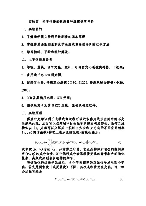
实验四 光学传递函数测量和透镜像质评价一. 实验目的1. 了解光学镜头传递函数测量的基本原理;2. 掌握传递函数测量和光学系统成像品质评价的近似方法3. 学习抽样、平均和统计算法。
二. 主要仪器及设备1. 导轨,滑块,调节支座,支杆,可调自定心透镜夹持器,干板夹;2. 多用途三色LED 面光源;3. 波形发生器,待测双凸透镜(Φ30,f120),待测双胶合透镜(Φ30,f90);4. CCD 及其稳压电源,CCD 光阑;5. 图像采集卡及其与CCD 连线,微机及相应软件。
三. 实验原理傅里叶光学证明了光学成像过程可以近似作为线形空间中的不变系统来处理,从而可以在频域中讨论光学系统的响应特性。
任何二维物体ψo (x , y )都可以分解成一系列x 方向和y 方向的不同空间频率(νx ,νy )简谐函数(物理上表示正弦光栅)的线性叠加:式中ψo (νx ,νy )为ψo (x , y )的傅里叶谱,它正是物体所包含的空间频率(νx ,νy )的成分含量,其中低频成分表示缓慢变化的背景和大的物体轮廓,高频成分则表征物体的细节。
当该物体经过光学系统后,各个不同频率的正弦信号发生两个变化:首先是调制度(或反差度)下降,其次是相位发生变化,这一综合过程可表为[])1(,)(2exp ),(),(o o y x y x y x d d y x i Ψy x ννννπννψ+=⎰⎰∞∞-∞∞-)2(),,(),(),(o i y x y x y x ΨH Ψνννννν⨯=)4( ,minmaxminmaxAAAAm+-=[]yxyxyxddiΨννηνξνπννηξψ)(2exp),(),(ii+=⎰⎰∞∞-∞∞-式中ψi(νx,νy)表示像的傅里叶谱。
H(νx,νy)称为光学传递函数,是一个复函数,它的模为调制度传递函数(modulation transfer function, MTF),相位部分则为相位传递函数(phase transfer function, PTF)。
实验二光学系统的PSF及MTF评价

实验二光学系统的PSF及MTF评价引言光学系统的性能评价是光学工程中非常重要的一部分,关注系统的成像质量和分辨率。
物体成像是通过光学系统中光线的折射、传播和调制来实现的,其中点扩散函数(Point Spread Function,PSF)和调制传递函数(Modulation Transfer Function,MTF)是常用的评价指标。
PSF反映了光学系统对点光源成像的能力,MTF则定性地描述了光学系统对不同频率光信号的调制能力。
本实验将通过计算和测量的方法,评价光学系统的PSF和MTF。
实验部分实验仪器和仪表1.准直仪:用于保证实验光路的准直。
2.光屏:放置在成像平面上,用于观察成像效果。
3.波长可调激光器:用于提供单色光源,可以调节波长以进行多波长光源实验。
4.干涉模块:用于产生干涉光源,用以模拟实际成像系统中的像差。
实验原理1.点扩散函数(PSF)PSF描述了光学系统对点光源的成像效果。
点光源在物平面的成像会存在衍射现象,其光强度分布将形成一个亮度最高的中心,周围呈现逐渐变暗的圆环状分布。
通过透镜对这一光斑进行调制,可以得到光斑的PSF,其数学表达式为:PSF(x,y)=,DFT(I(x,y)),^2其中,DFT表示二维离散傅里叶变换,I(x,y)表示点光源在成像平面上的光强分布。
2.调制传递函数(MTF)MTF衡量了光学系统对不同频率的光信号的传递能力,是评价光学系统成像分辨率的重要指标。
MTF可以通过PSF求取得到,其计算公式为:MTF=,DFT(PSF)其中,DFT表示二维离散傅里叶变换,PSF表示点光源的光斑。
实验步骤1.实验准备:将光学系统调整到准直状态,确保光路稳定。
2.测量单色光源的PSF:将单色光源对准成像平面,调整光源强度至适当水平,通过光屏观察光斑的形状。
使用相机或微观目镜记录光斑的图像,然后对图像进行数学处理,得到光斑的PSF。
3.测量多波长光源的PSF:使用波长可调激光器,分别设置不同的波长,进行相同的测量步骤,得到不同波长下的PSF。
调制传递函数
调制传递函数
调制传递函数(Modulation Transfer Function)MTF
一般通过光学系统的输出像的对比度总比输入像的对比度要差,这个对比度的变化量与空间频率特性有密切的关系。
把输出像与输入像的对比度之比称为调制传递函数,及MTF的定义是MFT=输出图像的对比度/输入图像的对比度,因为输出图像的对比度总小于输入图像的对比度,所以MFT值介于0~1之间。
调制传递函数可用于表示光学系统的特征,MTF越大,表示系统的成像质量越好。
调制传递函数(MTF)表示调制度与图像内每毫米线对数之间的关系,是所有光学系统性能判断中最全面的判据,特别是对于成像系统。
一个图案强度按正弦规律变化的周期性目标由待测镜头成像后,像面处的图案强度是由相差、衍射、装配和校准误差以及其他因素,像质有点退化,亮暗成度不如初始。
调制度就是最大强度与最小强度之差与最大强度与最小强度之和的比。
MTF是像的调制度与物的调制度之比。
它是空间频率的函数,空间频率通常以1p/mm的形式表示。
MTF说明物的调制度被镜头传递到像的情况。
MTF的计算通常使用径向靶条和切向靶条,且切向靶条彼此垂直。
然而,对于具有像素特性的阵列探测器,分辨力靶条应与像素行和列相一致,使用垂直靶条和水平靶条要比使用径向和切向靶条更为合适。
IS-200传函仪的测量MTF数据分析
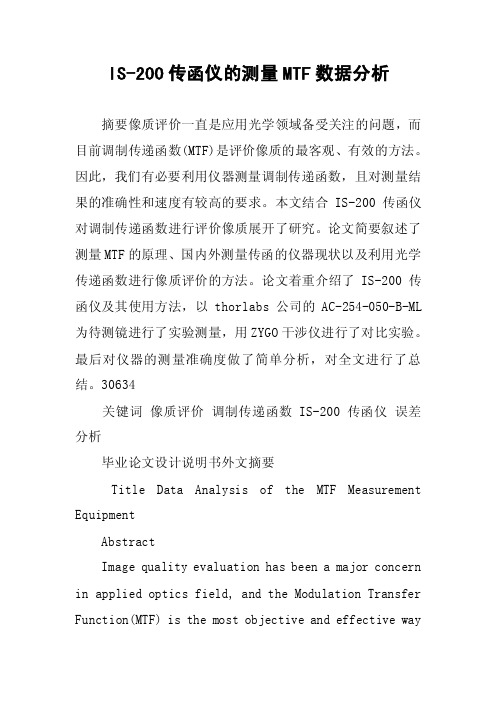
IS-200传函仪的测量MTF数据分析摘要像质评价一直是应用光学领域备受关注的问题,而目前调制传递函数(MTF)是评价像质的最客观、有效的方法。
因此,我们有必要利用仪器测量调制传递函数,且对测量结果的准确性和速度有较高的要求。
本文结合IS-200传函仪对调制传递函数进行评价像质展开了研究。
论文简要叙述了测量MTF的原理、国内外测量传函的仪器现状以及利用光学传递函数进行像质评价的方法。
论文着重介绍了IS-200传函仪及其使用方法,以thorlabs公司的AC-254-050-B-ML 为待测镜进行了实验测量,用ZYGO干涉仪进行了对比实验。
最后对仪器的测量准确度做了简单分析,对全文进行了总结。
30634关键词像质评价调制传递函数 IS-200传函仪误差分析毕业论文设计说明书外文摘要Title Data Analysis of the MTF Measurement EquipmentAbstractImage quality evaluation has been a major concern in applied optics field, and the Modulation Transfer Function(MTF) is the most objective and effective wayto evaluate the image quality. Therefore, it is necessary to use instruments measure the MTF, and we have a high requirement for the measurement accuracy and speed of the instruments. Based on the IS-200 measurement equipment, the thesis studied image quality evaluation using the optical transfer function. This paper briefly describes the principles of measuring MTF, the domestic and overseas present situation of instruments measuring MTF and image quality evaluation using MTF. Besides, the thesis specifically introduces the IS-200 instrument and how it works. The thorlabs's AC-254-050-B-ML under test,the experiment was carried out. The contrast experiment using the ZYGO interferometer is conducted. Finally, a simple analysis of instrument measurement accuracy was done and the full text was summarized .源自Keywords image quality evaluation modulation transfer function IS-200 measurement equipment error analysis目次1 引言 11.1 MTF发展史 11.2 传函仪发展状况 21.3 课题研究内容 32 MTF介绍 42.1 调制度(对比度) 42.2 点扩散函数和线扩散函数 42.3 调制传递函数基本概念 42.4 MTF评价像质 53 传函仪原理 74 IS-200传函仪使用说明 84.1 IS-200传函仪系统构成 84.2 Matrix软件 134.3 IS-200传函仪快捷使用说明 184.4 注意事项 195 实验测量 205.1 AC-254-050-B-ML待测镜 205.2 IS-200传函仪测量 225.3 ZYGO干涉仪测量 256 MTF测量数据与误差分析 266.1 MTF测量数据 266.2 传函仪误差分析 316.3 不同频率焦点位置测试结果差异 36结论 37致谢 39参考文献401 引言现如今,人们获取各种各样信息方式很多,但是其中的80%以上是通过视觉器官(眼睛)得到的。
光学传递函数的测量和像质评价

光学传递函数的测量和像质评价引言光学传递函数是表征光学系统对不同空间频率的目标函数的传递性能,是评价光学系统的指标之一。
它将傅里叶变换这种数学工具引入应用光学领域,从而使像质评价有了数学依据。
由此人们可以把物体成像看作光能量在像平面上的再分配,也可以把光学系统看成对空间频率的低通滤波器,并通过频谱分析对光学系统的成像质量进行评价。
到现在为止,光学传递函数成为了像质评价的一种主要方法。
一、实验目的了解光学镜头传递函数的基本测量原理,掌握传递函数测量和成像品质评价的近似方法,学习抽样、平均和统计算法,熟悉光学软件的应用。
二、基本原理光学系统在一定条件下可以近似看作线性空间中的不变系统,因此我们可以在空间频率域来讨论光学系统的响应特性。
其基本的数学原理就是傅里叶变换和逆变换,即:dxdy y x i y x )](2exp[,ηξπψηξψ+-=⎰⎰)(),( (1) ηξηξπηξψψd d y x i y x )](2exp[),(),(+=⎰⎰ (2)式中),(ηξψ是),(y x ψ的傅里叶频谱,是物体所包含的空间频率),(ηξ的成分含量,低频成分表示缓慢变化的背景和大的轮廓,高频成分表示物体细节,积分范围是全空间或者是有光通过空间范围。
当物体经过光学系统后,各个不同频率的正弦信号发生两个变化:首先是调制度(或反差度)下降,其次是相位发生变化,这一综合过程可表为),(),(),(ηξηξψηξφH ⨯= (3)式中),(ηξφ表示像的傅里叶频谱。
),(ηξH 成为光学传递函数,是一个复函数,它的模为调制度传递函数(modulation transfer function, MTF ),相位部分则为相位传递函数(phase transfer function, PTF )。
显然,当H =1时,表示象和物完全一致,即成象过程完全保真,象包含了物的全部信息,没有失真,光学系统成完善象。
由于光波在光学系统孔径光栏上的衍射以及象差(包括设计中的余留象差及加工、装调中的误差),信息在传递过程中不可避免要出现失真,总的来讲,空间频率越高,传递性能越差。
红外成像系统的调制传递函数测试
红外成像系统的调制传递函数测试摘要:本文介绍了红外成像系统的调制传递函数测试方法,包括传统的测试方法和基于数字信号处理的测试方法。
传统的测试方法包括基于光学系统的测试方法和基于信号处理系统的测试方法。
基于数字信号处理的测试方法包括基于频域分析的测试方法和基于时域分析的测试方法。
本文还介绍了测试结果的分析和应用。
关键词:红外成像系统;调制传递函数;频域分析;时域分析一、引言红外成像系统是一种能够在低光照条件下进行成像的系统,可以用于军事、安防、医疗等领域。
在红外成像系统中,调制传递函数是一个重要的参数,它描述了系统对输入信号的响应。
因此,测试红外成像系统的调制传递函数是非常必要的。
传统的测试方法包括基于光学系统的测试方法和基于信号处理系统的测试方法。
基于光学系统的测试方法是通过对系统进行正弦光栅测试,得到系统的调制传递函数。
基于信号处理系统的测试方法是通过对系统进行正弦信号测试,得到系统的调制传递函数。
这两种方法都有一些缺点,如测试精度不高、测试时间长等。
基于数字信号处理的测试方法是一种新的测试方法,它可以通过对系统输出信号的频域或时域进行分析,得到系统的调制传递函数。
这种方法具有测试精度高、测试时间短等优点,因此在实际应用中得到了广泛的应用。
本文将介绍红外成像系统的调制传递函数测试方法,包括传统的测试方法和基于数字信号处理的测试方法。
并将分析测试结果的应用。
二、传统的测试方法1、基于光学系统的测试方法基于光学系统的测试方法是通过对系统进行正弦光栅测试,得到系统的调制传递函数。
测试原理如下图所示: 其中,$I_0$为入射光强度,$I_1$为透过光栅后的光强度,$I_2$为透过系统后的光强度,$T$为光栅周期,$lambda$为光波长,$f$为系统的空间频率,$MTF(f)$为系统的调制传递函数。
- 1、下载文档前请自行甄别文档内容的完整性,平台不提供额外的编辑、内容补充、找答案等附加服务。
- 2、"仅部分预览"的文档,不可在线预览部分如存在完整性等问题,可反馈申请退款(可完整预览的文档不适用该条件!)。
- 3、如文档侵犯您的权益,请联系客服反馈,我们会尽快为您处理(人工客服工作时间:9:00-18:30)。
How to Measure Modulation Transfer Function http://harvestimaging.com/blog/?p=1294 How to Measure Modulation Transfer Function (1)
In a simple wording, the modulation transfer function or MTF is a measure of the spatial resolution of an imaging component. The latter can be an image sensor, a lens, a mirror or the complete camera. In technical terms, the MTF is the magnitude of the optical transfer function, being the Fourier transform of the response to a point illumination. The MTF is not really the most easiest measurement that can be done on an imaging system. Various methods can be used to characterize the MTF, such as the “slit image”, the “knife edge”, the “laser-speckle technique” and “imaging of sine-wave patterns”. It should be noted that all method listed, except the “laser-speckle technique, measure the MTF of the complete imaging system : all parts of the imaging system are included, such as lens, filters (if any present), cover glass and image sensor. Even the effect of the processing of the sensor’s signal can have an influence on the MTF, and will be include in the measurement. In this first MTF-blog the measurement of the modulation transfer function based on imaging with a sine-wave pattern will be discussed. It should be noted that in this case dedicated testcharts are used to measure the MTF, but the pattern on the chart should sinusoidally change between dark parts and light parts. In the case a square-wave pattern is used, not the MTF but the CTF (= Contrast Transfer Function) will be measured. And the values obtained for the CTF will be larger than the ones obtained for the MTF. The method described here is based on the work of Anke Neumann, written down in her MSc thesis “Verfahren zur Aufloesungsmessung digitaler Kameras”, June 2003. The basic idea is to use a single testchart with a co-called Siemens-star. An example of such a testchart is illustrated in Figure 1. Figure 1 : Output image of the camera-under-test observing the Siemens star. (Without going further into detail, the testchart contains more structures than used in the reported measurement performed for the MTF.) The heart of the testchart is the Siemens star with 72 “spokes”. As can be seen the distance between the black and white structures on the chart is becoming larger if one moves away from the center of the chart. In other words, the spatial frequency of the sinusoidal pattern is becoming lower at the outside of the Siemens star, and is becoming higher closer to the center of the Siemens star. Around the center of the Siemens star, the spatial frequency of the sinusoidal pattern is even too high to be resolved by the camera-under-test and aliasing shows up. In the center of the Siemens star a small circle is included with 2 white and two black quarters. These are going to play a very important role in the measurements. The measurement procedure goes as follows : 1. Focus the image of the Siemens star, placed in front of the camera, as good as possible on the imager. Try to bring the Siemens star as close as possible to the edges (top and bottom) of the imager, 2. Shoot an image of the testchart (in the example described here, 50 images were taken and averaged to limit the temporal noise). In principle, these two steps is all one needs to be able to measure/calculate the MTF. But to obtain a higher accuracy of the measurements, the following additional steps might be required : 1. Cameras can operate with or without a particular offset corrected/added to the output signal. For that reason it might be wise to take a dark reference frame to measure the offset and dark signal (including its non-uniformities) for later correction. In the experiments discussed here, 50 dark frames were taken and averaged to minimize the temporal noise. 2. The data used in the measurement is coming from a relatively large area of the sensor and is relying on an uniform illumination of the complete Siemens star. Moreover, the camera is using a lens and one has to take into account the lens vignetting or intensity fall-off towards the corners of the sensor. For that reason a flat-fielding operation might be needed : take an image of a uniform test target, and use the data obtained to create a pixel gain map. In the experiments discussed her, 50 flat field images were taken and averaged to minimize the temporal noise. 3. The camera under test in this discussion delivers RAW data, without any processing. If that was not the case it would have been worthwhile to check the linearity of the camera (e.g. use of a gamma correction) by means of the grey squares present on the testchart as well. Taken all together the total measurement sequence of the MTF characterization is then composed of : 1. Shoot 50 images of the focused testchart, and calculate the average. The result is called : Image_MTF, 2. Shoot 50 flat field images with the same illumination as used to shoot the images of the focused testchart, and calculate the average image of all flat field images. The result is called :Image _light, 3. Shoot 50 images in dark, and calculate the average image of all dark image. The result is called Image_dark, 4. Both Image_MTF and Image_light are corrected for their offset and dark non-uniformities by subtracting Image_dark, 5. The obtained correction (Image_light – Image_dark) will be used to create a gain map for each pixel, called Image_gain, 6. The obtained correction (Image_MTF – Image_dark) will be corrected again for any non-uniformities in pixel illumination, based on Image_gain. If this sequence is followed, an image like the one shown in Figure 1 can be obtained. 1. Next the pixel coordinates of the center of the testchart need to be found. This can be done manually or automatically. The latter is done in this work, based on the presence of the 4 quadrants in the center of the testchart. 2. Once the centroid of the testchart is known, several concentric circles are drawn with the centroid of the testchart as their common center. An example of these concentric circles on top of the testchart is shown in Figure 2.