数学分析 高等数学 微积分 英语课件 上海交通大学Chapter5b
《高等数学B》课程教学大纲
合重要作用,了解本学科中学教学领域的一些新研究成果和教学方法;掌握教育学、心理学和数学教育的基本理论,熟悉中小学教学技能以及教育法规;学习人类文明进步与文化发展的通识知识。
具有整合数学、教育技术、教育学、心理学及本学科的知识和教育技术并进行知识与技能重构的能力。
2、32.4教学能力具备良好的数学素养,深入理解高等数学并掌握的基本理论和方法,并能获得较强的逻辑推理能力和抽象思维能力。
初步掌握高等数学的基本思想方法,具有分析问题、解决实际问题等基本能力;具有较强的独立学习能力和创新思维方式,懂得教育教学基本规律,掌握现代教育教学、心理学的基本理论。
课程学习目标1、2、3三、课程各要素与课程学习目标的对应关系及达成度分析(一)课程教学内容、教学目标、学时分配与课程学习目标的对应关系第一章函数、极限与连续(可支撑课程学习目标1、2、3)1 . 教学目的和要求掌握集合及其运算、邻域、基本初等函数及初等函数的基本概念;数列、函数极限的基本概念、求极限的基本方法及极限的性质及其证明;两个重要极限的应用;无穷大与无穷小的基本概念及其关系、无穷小阶的比较;函数的连续性及其性质。
2 . 教学内容第1.1节:集合与函数第1.2节:数列极限的定义与计算第1.3节:函数极限的定义与计算第1.4节:极限性质第1.5节:两个重要极限第1.6节:无穷小与无穷大第1.7节:函数的连续性及其性质3 . 重点:数列极限的概念及性质,函数极限的概念与性质,函数极限与数列极限的关系,极限存在准则两个重要极限和闭区间上连续函数的性质4 . 难点:难点是数列极限与函数极限的概念。
5 . 参考习题:习题1-1:第1(4)、2、3、4题(3、5、6)、6(2、5-8)、9-11、14-15题习题1-2:第2(2-10)、3题习题1-3:第1(3、5、6、8-14)、2-4题习题1-5:第1-3(1)题习题1-6:第2-4题习题1-7:第1-12题6 . 学时:20学时第二章一元函数微分学及其应用(可支撑课程学习目标1、2、3)1 . 教学目的和要求掌握导数的基本概念及基本求导公式;求导数、高阶导数的方法与技巧;掌握微分的基本概念及微分的求法;掌握微分中值定理的内容、证明方法及其应用;熟练掌握函数单调性的判别方法、求函数的单调区间与极值、凹凸区间与拐点,求函数的最值、曲率,并可以解决一些简单的实际问题2 . 教学内容第2.1节:导数的概念及基本求导公式第2.2节:导数的计算法则第2.3节:微分的概念应用第2.4节:微分中值定理及其应用第2.6节:函数的性态与图形第2.7节:微分学的实际应用3.重点:导数的定义,函数的求导法则及函数的微分, 微分中值定理,洛必达法则,函数的单调性与凹凸性,函数的极值与最值;4.难点:复合函数的求导法则,反函数及参数方程求高阶导数,微分中值定理及其应用,函数图形的描绘。
托马斯微积分课件5.3 Lengths of Plane Curves
5.1 Volumes by Slicing and Rotation About an Axis 5.2 Modeling Volume Using Cylindrical Shells 5.3 Lengths of Plane Curves
目录
上页
下页
返回
结束
Supposed that a curve can be described by the parametric equations
目录
上页
下页
返回
结束
目录
上页
下页
返回
结束
Exercises
P420 3, 15, 16.
目录
上页
下页
返回
结束
5.4 Springs, Pumping and Lifting 5.5 Fluid Forces
5.6 Moments and Centers of Mass
目录 上页 下页 返回 结束
5.3
Lengths of Plane Curves
(平面曲线长度)
目录
上页
下页
返回
结束
A smooth curve (光滑曲线)
lim Lk lim 1 f ck xk P 0
2
n
n
k 1
P 0
k 1
目录
上页
下页
返回
结束
目录
上页
下页
返回
结束
Solution.
目录
上页
下页
返回
结束
Solution.
上海立信会计金融高等数学 b-微积分
高校数学课程是大学教育中不可或缺的一部分,而高等数学 b-微积分作为数学专业的基础课程之一,对于培养学生的数学思维和分析能力具有重要意义。
作为我国知名的高校之一,上海立信会计金融高等数学 b-微积分课程在教学内容、教学方法以及学习效果等方面都具有一定的特色和优势。
一、教学内容全面上海立信会计金融高等数学 b-微积分课程的教学内容全面,包括微积分的基本概念、导数与微分、积分与微分方程等内容,涵盖了微积分的各个重要知识点,并且教学内容与数学专业的发展趋势和实际应用密切相关,有助于学生全面系统地掌握微积分的基础知识和方法,为将来深入学习数学以及从事相关领域的工作打下坚实的基础。
二、教学方法灵活多样在教学方法上,上海立信会计金融高等数学 b-微积分课程注重灵活多样的教学方式。
除了传统的课堂教学外,还注重引导学生进行实际应用和实验,通过案例分析和解决实际问题的方式,深化学生对微积分理论知识的理解和应用能力。
教师会根据学生的学习特点和需求,采用不同的教学方法和手段,例如小组讨论、课外辅导等,使学生在思维方式和学习方法上得到全面提高。
三、学习效果显著上海立信会计金融高等数学 b-微积分课程在学习效果上表现显著。
通过对学生的学习情况进行全面的跟踪和评估,教师及时发现学生的学习困难和问题,采取相应的措施进行指导和辅导,使学生的学习效果得到进一步提高。
学校还注重对学生的认知能力、动手能力和创新能力的培养,使学生在学习微积分的过程中获得综合能力的提升,为其未来的学习和发展奠定坚实基础。
四、教学团队实力雄厚上海立信会计金融高等数学 b-微积分课程的教学团队实力雄厚,拥有一支高素质的教师队伍。
教师们既具有扎实的数学理论基础,又具备丰富的教学经验和实践能力,能够根据学生的学习特点和需求,灵活运用教学手段和方法,使得教学过程生动有趣,引导学生主动参与学习,达到教学的最佳效果。
在总体上看,上海立信会计金融高等数学 b-微积分课程具有教学内容全面、教学方法灵活多样、学习效果显著和教学团队实力雄厚等优点。
微积分讲义Chap 1 Completeness axiom of R
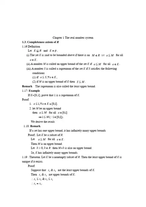
Chapter 1 The real number system1.3. Completeness axiom of R1.16 DefinitionLet R E ⊆ and φ≠E .(i).The set E is said to be bounded above if there is an R M ∈ s.t M a ≤ for allE a ∈.(ii).A number M is called an upper bound of the set E if M a ≤ for all E a ∈. (iii).A number S is called a supremum of the set E if S satisfies the followingconditions(1) if E a S a ∈∀≤,,(2) if M is an upper bound of E then M S ≤.Remark The supremum is also called the least upper bound.1.17: ExampleIf E=[0,1], prove that 1 is a supremum of E .Proof.1. ]1,0[,1=∈∀≤E a a .2. let M be an upper boundthen M a ≤ for all ]1,0[∈a])1,0[1(1∈≤⇒ M .We derive the result.1.18: RemarkIf a set has one upper bound, it has infinitely many upper boundsProof:. Let E be a subset of R .Let M a ≤ for all E a ∈.Then M is an upper bound.Let R b b ∈>,0 then M+b is also an upper bound.So, E has infinitely many upper bounds.1.19 . Theorem. Let E be a nonempty subset of R . Then the least upper bound of E is unique if it exists.Proof.Suppose that 21&s s are the least upper bounds of E.Then 21&s s are upper bounds of E .1221&s s s s ≤≤∴21s s =∴.NotationThe supremum is also called least upper bound . We use sup E to denote the supremum of nonempty set E .1.20. Theorem [Approximation property]E E R E sup and ,,φ≠⊆exists. Then E a ∈>∀an is there ,0ε s.t E a E sup sup ≤<-ε.Proof:. Suppose the conclusion is false. There is an 0>ε such that.,sup E a E a ∈∀-≤ε.ε-∴E sup is an upper bound.→←≥-⇒E E sup sup ε0>εE a ∈∃∴ s.t E a E sup sup ≤<-ε1.21. TheoremIf N E ⊆ has a supremum, then E E ∈supProof.Let supE=s.By Approximation property, there E x ∈∃0 s.t s x s ≤<-01.If s x =0 then E E ∈sup is obvious.If s x s <<-01, thenE x ∈∃1 s.t 001100x s x x s x x -≤-<⇒≤<.1. 1,0101≥-⇒∈x x N x x .2. 1)1(1,0101=--<-⇒->≥s s x x s x x s .It is a contradiction.E E ∈∴sup● [Complete axiom of R ]Every nonempty subset E of R that is bounded above,then E has the least upper bound. .1.22 :[Archimedean Principle]N n b a R b a ∈∃⇒>∈0,,, s.t b<na.Proof:1. If b<a , then take n=1.2. If a<b , let };{b ka N k E ≤∈=.φ≠∴∈E E ,1 .⇒∈∀≤E k ab k ,E is bounded above. By Completeness of R , sup E exists.ba E E E E E >+∴∉+∴∈⇒)1(sup 1sup )21.1 Theorem by (suptake n=supE+11.23: Example.Let ,.......}41,21,1{=A and ,...}87,43,21{=B prove that supA=supB=1Proof.1. 1{;0}2n A n N or n =∈= 11,,0,1,2,..2n x x n ≥==. 1∴ is an upper bound.Let M be another bound..1sup 1210=∴=≥∴A M 2. };211{N n B n ∈-= N n n∈∀-≥,2111 1∴ is an upper bound of B.Let M be an upper bound of BTo show 1≥M .Suppose not 011>-⇒<⇒M MBy Archimedean principle, there exists N n ∈ such that M n-<11, M n-<∃⇒121 for some N n ∈. →←>-⇒-->-=-∴M M n n n n n 212)1(1212211 M is an upper bound. 1≥∴M1sup =∴B● [Well-Order Principle]⇒≠⊆φE N E ,E has a least element(ie.E a ∈∃ s.t E x x a ∈∀≤,)1.24. Theorem (Density of rational)Let R b a ∈, satisfy a<b , then there is a rationalnumber c s.t a<c<b.Proof:Let N n a b n∈-<,1(by Archimedean Principle). 1. If b>0, let }.;{nk b N k E ≤∈= By Archimedean Principle φ≠⇒E .By Well-Order Principle ⇒E has a least element, says 0k . .)..(1:0b n m e i E m k m <∉⇒-=∴ Let nm q =. We must show that a<q<b.q<b is obvious, now we show that a<q....11)(00b q a a q q n k n n k a b b a <<∴>∴=-=-<--=2. If b<0, then0>∃k , k is a natural number s.t b+k>0.Q c ∈∃∴ s.t a+k<c<b+kQk c Q c bk c a ∈-⇒∈<-<∴ie. There is a rational number between a & b.1.27. Definition.φ≠⊆E R E ,.1. s is called a lower bound of E if E x s x ∈∀≥,.In the case, E is called bounded below2.t is called the greatest lower bound of Eif1.Extx∈∀≥,,2. If M is a lower bound of E then tM≤.3.E is bounded if ExMx∈∀≤,for some M>0. (i.e. E is bounded above and below.)●Let E be a set of R. We define };{ExxE∈-=-.1.28. Theoremφ≠⊆ERE,.1.sup E exists ⇔inf(-E) existsin fact supE= -inf(-E)2.inf E exists⇔sup(-E) existsin fact inf E= -sup(-E)Proof:1.""⇒supE exists.Now we show that –supE=inf(-E).Show that 1.-sup E is a lower bound of –E.2. if s is a lower bound of EsE sup-≤⇒-.1.Esupis an upper bound of EExExExEx∈∀-≥-⇒∈∀≤∴,sup,supEsup-∴is a lower bound of –E2. Suppose that s is a lower bound of -ESuppose not EsEs supsup<-⇒->⇒on the other hands xE xs x-≤∴∈∀≥-,Hence, -s is a upper bound of E→←By 1.& 2, EEE sup)inf(&)inf(-=-∃-.The proof of converse is similar.Remark. The largest lower bound is also called infimum. Remark. The completeness axiom of R is equivalent to“ Every nonempty, bounded below subset of R has the infimum”.1.29. Theorem.inf inf ,sup sup ,,A B A B B A R B A ≤≥⇒≠⊆⊆φif B B inf and sup exist.Hence, B A A B sup sup inf inf ≤≤≤Proof:1. suppose sup B exists.,sup .,sup A x B x B A B x B x ∈∀≤∴⊆∈∀≤∴A ∴ is bounded above & supB is an upper bound of ABy complete axiom of R, .sup sup &sup B A A ≤∃2. S ppose that inf B exists..,inf ,inf A x B x B A Bx B x ∈∀≥∴⊆∈∀≥∴A ∴ is bounded below & infB is an lower bound of A.By complete axiom of R, B A A inf inf &:inf ≥∃.Def:sup ,inf φφ=-∞=∞1.4 Functions, countability and the algebra of sets.DefinitionLet A & B be two sets of R.A function f is a relation between A &B s.t f assigns each element x of A to aunique By∈Definition:f→ABf is called 1-1 if )x≠y⇒≠f(yx)(fDef::f→BAf is called onto if A∈∀,s.t f(x)=y∃xBy∈Definition 1.34:Let E be s a set of R.1. E is said be finite if φ&∃}...3,2,1{∈.....},2,1{:=n→E or EnnNfs.t f is 1-1 & onto.2. E is called countably infinite if E∃:s.t f is 1-1 & onto.Nf→3. E is called countable if E is finite or countably infinite.4. E is called uncountable if E is not countable1.35. Theorem .The open interval (0,1) is uncountablePf:Suppose (0,1) is countable.Then there is a list for (0,1) says.....................................................................0............................................................................0.........0.........0321333231323222121312111n n n n a a a a a a a a a a a a a a a a ==== Let .......0321ααα=x where {=k α10==k k αα .1f ,1if ≠=kk kk a i a kk k a ≠∴α x ∴ is not in this list →← (0,1) is uncountable1.37. TheoremB B A ,⊆ is countable A ⇒ is countable1.38 Theoremn A A A ,......,21 are countable. },:{:1N j A x x A A E j j j N j j∈∈===∞=∈ .If j A is countable for E N j ⇒∈ is countable.。
(完整)上海交通大学年数学分析
上海交通大学2007年数学分析一、(每小题6分,共24分)判断下列命题的真伪,正确的命题请简要证明,错误的命题举出反例.1、若{}n x 为有界数列,记{}sup n x β=,则{}n x 必有子列{}k n x ,使得lim k n k x β→∞=. 2、若函数()f x 和()g x 在[),a +∞上一致连续,则()()f x g x 在[),a +∞上一致连续.3、若函数列{}()n f x 在区间(],a c 和[),c b 上一致收敛,那么{}()n f x 在(),a b 上一致收敛。
4、若级数1n n a ∞=∑绝对收敛,而lim 1n n b →∞=,则1n n n a b ∞=∑绝对收敛.二、(每小题8分,共64分)计算下列各题。
1、计算极限2sin sin sin lim()121n n n n n n n n πππ→∞++++++. 2、计算极限112112ln(1sin(1))lim()11x x x e x x e -→-++-+-+。
3、设221()arctan 1x f x x+=-,求高阶导数()()n f x ,其中n N ∈. 4、设广义积分20sin()px I dx x +∞=⎰(1p >-)。
试问p 为何值时广义积分绝对收敛,p 为何值时广义积分条件收敛?5、设()f x 在闭区间[]0,1上连续且恒正,20()n n a x f x dx =⎰。
求函数项级数0n n n x a ∞=∑的收敛域。
6、设二元函数222222,0(,)0,0x y x y x y f x y x y α⎧+≠⎪+=⎨⎪+≠⎩,0α>.问α为何值时函数(,)f x y 在点(0,0)处可微?.7、计算三重积分3()arctan I y z zdxdydz Ω=-⎰⎰⎰,其中Ω是由曲面2221()2x y z R +-=,0z =,z h =所围成的立体。
数学分析(一):一元微积分 南京大学 5 第五章微分学的应用 (5.9.1) Taylor展开和近似计算

一元微积分与数学分析—T aylor展开和近似计算梅加强南京大学数学系在前一单元,我们证明了圆周率π是无理数.在实际应用中,我们往往需要用有限小数(有理数)代替无理数参与计算.在前一单元,我们证明了圆周率π是无理数.在实际应用中,我们往往需要用有限小数(有理数)代替无理数参与计算.问题1:怎样尽可能精确地用有理数去逼近π?在前一单元,我们证明了圆周率π是无理数.在实际应用中,我们往往需要用有限小数(有理数)代替无理数参与计算.问题1:怎样尽可能精确地用有理数去逼近π?阿基米德(前287年–前212年)利用穷竭法得到圆周率的近似值22/7.在前一单元,我们证明了圆周率π是无理数.在实际应用中,我们往往需要用有限小数(有理数)代替无理数参与计算.问题1:怎样尽可能精确地用有理数去逼近π?阿基米德(前287年–前212年)利用穷竭法得到圆周率的近似值22/7.刘徽(约公元225年–公元295年)提出了“割圆术”:“割之弥细,所失弥少,割之又割,以至于不可割,则与圆周合体而无所失矣.”在前一单元,我们证明了圆周率π是无理数.在实际应用中,我们往往需要用有限小数(有理数)代替无理数参与计算.问题1:怎样尽可能精确地用有理数去逼近π?阿基米德(前287年–前212年)利用穷竭法得到圆周率的近似值22/7.刘徽(约公元225年–公元295年)提出了“割圆术”:“割之弥细,所失弥少,割之又割,以至于不可割,则与圆周合体而无所失矣.”利用割圆术,刘徽算出圆周率的近似值3.14.阿基米德和刘徽图1:阿基米德图2:刘徽达到精确的程度.于是他进一步精益钻研,去探求更精确的数值,最终得出3.1415926<π<3.1415927.于是他进一步精益钻研,去探求更精确的数值,最终得出3.1415926<π<3.1415927.祖冲之还采用了两个分数值的圆周率,一个是355/113≈3.1415927,这一个数比较精密,所以祖冲之称它为“密率”.另一个是22/7≈3.14,这一个数比较粗疏,所以祖冲之称它祖冲之所取得的成就是很了不起的.如果沿用他的方法求更精确的近似值极为困难.祖冲之所取得的成就是很了不起的.如果沿用他的方法求更精确的近似值极为困难.问题2:还有其他方法计算圆周率吗?祖冲之所取得的成就是很了不起的.如果沿用他的方法求更精确的近似值极为困难.问题2:还有其他方法计算圆周率吗?微积分发明出来以后人们很快发现可以用来计算圆周率的近似值.祖冲之所取得的成就是很了不起的.如果沿用他的方法求更精确的近似值极为困难.问题2:还有其他方法计算圆周率吗?微积分发明出来以后人们很快发现可以用来计算圆周率的近似值.我们用T aylor展开来计算π.回顾arctan x的Maclaurin展开arctan x=x−x33+x55−x77+···,x∈[−1,1].取x=1,左边等于π/4.不过,右边收敛得很慢,还不能直接用于π的计算.祖冲之所取得的成就是很了不起的.如果沿用他的方法求更精确的近似值极为困难.问题2:还有其他方法计算圆周率吗?微积分发明出来以后人们很快发现可以用来计算圆周率的近似值.我们用T aylor展开来计算π.回顾arctan x的Maclaurin展开arctan x=x−x33+x55−x77+···,x∈[−1,1].取x=1,左边等于π/4.不过,右边收敛得很慢,还不能直接用于π的计算.注意到当|x|比较小的时候,右边收敛速度就比较快了.基本的想法就是用若干个注意到tan(u+v)=tan u+tan v 1−tan u tan v,当u=arctan(1/5)时,就有tan(2u)=2/51−(1/5)2=5/12,tan(4u)=10/121−(5/12)2=120/119.因此tan4u−π/4=120/119−11+120/119=1/239,注意到tan(u+v)=tan u+tan v 1−tan u tan v,当u=arctan(1/5)时,就有tan(2u)=2/51−(1/5)2=5/12,tan(4u)=10/121−(5/12)2=120/119.因此tan4u−π/4=120/119−11+120/119=1/239,这就得到等式π4=4arctan15−arctan1239.(1)它可以改写为如下的Machin公式π=16∞n=0(−1)n(2n+1)52n+1−4∞n=0(−1)n(2n+1)2392n+1,(2)这个公式已经可用于实际的计算了.它可以改写为如下的Machin公式π=16∞n=0(−1)n(2n+1)52n+1−4∞n=0(−1)n(2n+1)2392n+1,(2)这个公式已经可用于实际的计算了.1706年,Machin用这个公式将π计算到了小数点后100位.类似地,我们可以得到等式2arctan110=arctan15+arctan1515,从而有π=32arctan 110−4arctan 1239−16arctan1515=32 110−131103+151105−171107+191109−11111011 +δ1−4 1239−1312393 −δ2−16 1515−1315153−δ3,从而有π=32arctan 110−4arctan 1239−16arctan1515=32 110−131103+151105−171107+191109−11111011 +δ1−4 1239−1312393 −δ2−16 1515−1315153−δ3,其中3213×10−13−3215×10−15<δ1<3213×10−13,因此0.24×10⁻¹²<δ1<0.25×10⁻¹².同理,1.02×10−12<δ2<1.03×10−12,0.08×10−12<δ3<0.09×10⁻¹²,因此−0.88×10⁻¹²<δ1−δ2−δ3<−0.85×10⁻¹².同理,1.02×10−12<δ2<1.03×10−12,0.08×10−12<δ3<0.09×10⁻¹²,因此−0.88×10⁻¹²<δ1−δ2−δ3<−0.85×10⁻¹².另一方面,π≈32 110−131103+151105−171107+191109−11111011−4 1239−1312393 −16 1515−1315153=3.14159265359066...总之得到3.14159265358978<π<3.14159265358982,近似值精确到了小数点后第12位.如何更快地精确计算π是一个很有意思的数学问题.1914年,印度天才数学家Ramanujan得到了一系列公式,其中一个为1π=2√29801∞k=0(4k)!(k!)444k1103+26390k994k,(3)这个公式的每一项可提供π的大约8位有效数字.如何更快地精确计算π是一个很有意思的数学问题.1914年,印度天才数学家Ramanujan得到了一系列公式,其中一个为1π=2√29801∞k=0(4k)!(k!)444k1103+26390k994k,(3)这个公式的每一项可提供π的大约8位有效数字. 1989年,Chudnovsky兄弟发表了公式1π=12∞k=0(−1)k(6k)!(3k!)(k!)313591409+545140134k6403203k+3/2,(4)这个公式的每一项可提供π的大约15位有效数字.另一方面,1995年,Bailey,Borwein和Plouffe发现了下面的公式π=∞k=048k+1−28k+4−18k+5−18k+6116k,(5)他们利用这个公式证明了,在2进制下可以直接计算π的第n位小数而无需知道其前n−1位小数的值.另一方面,1995年,Bailey,Borwein和Plouffe发现了下面的公式π=∞k=048k+1−28k+4−18k+5−18k+6116k,(5)他们利用这个公式证明了,在2进制下可以直接计算π的第n位小数而无需知道其前n−1位小数的值.人们利用已经发现的这些算法可以在计算机上进行π的快速高精度计算,这也成为了检验计算机运行速度的初步手段.。
上海财经大学英语高数课件05
Example 2: Find the area under the parabola y=x2+1 from 0 to 2.
Solution Since y=x2+1 is continuous, the limit (1) must exist for all possible partition P of the interval [a, b] as long as ||P|| 0. To simplify things let us take a regular partition. Then the partition points are x0=0, x1=2/n, x2=4/n, … , xi=2i/n, … , xn=2n/n=2
a
f ( x)dx lim
|| P|| 0
f ( x i )xi i 1
n
if this limit exists. If the limit does exist, then f is called integrable on the interval [a, b]. Note 1:
So the norm of P is
||P||=2/n Let us choose the point xi to be the right-hand endpoint:
xi = xi=2i/n
By definition, the area is
机动 目录 上页 下页 返回 结束
i 2 14 A lim f ( xi )xi lim f ( 2 ) n n 3 || P|| 0 i 1 n i 1
sin b
/section 5.2 end
上交大高等数学
上交大高等数学引言高等数学是大学数学教育中的一门重要课程,而上海交通大学(以下简称上交大)的高等数学课程则是学生理工类专业不可或缺的一部分。
本文旨在介绍上交大高等数学课程的主要内容、教学方法以及学习资源,以便学生更好地了解和应对该门课程。
课程概述上交大的高等数学课程主要分为两个学期,分别为上学期的高等数学A和下学期的高等数学B。
这门课程是一门基础课程,为学生提供了数学思维和分析问题的基本方法。
课程的主要内容包括微积分的基本概念和基本运算、不定积分与定积分、多元函数微分学、多元函数积分学等。
教学方法上交大高等数学课程注重理论与实践相结合的教学方法,以培养学生的数学思维和解决实际问题的能力为目标。
在教学中,教师会通过讲解、示范、练习和实例分析等方式,引导学生掌握数学知识和技能。
此外,学生也会参与小组讨论和课堂演示,以培养团队合作和表达能力。
学习资源为了帮助学生更好地学习高等数学,上交大提供了丰富的学习资源。
首先,学生可以获得教师精心编写的教材和讲义,这些教材详细介绍了每个章节的知识点和解题技巧。
其次,学生还可以参加教师组织的习题讲解课程或者预习课程,以巩固所学内容。
此外,上交大还建立了一个在线学习平台,学生可以在上面找到课程相关的视频教程、习题和答案等资源。
学习建议对于上交大高等数学课程,以下是一些建议,帮助学生更好地学习和掌握该门课程:1.当及时复习与巩固:高等数学是一门理论与实践相结合的课程,所以学生需要在学习新知识后及时复习,并通过练习题来巩固所学内容。
2.积极参与课堂讨论:课堂讨论是学生与教师和同学们互动交流的重要机会,可以帮助学生更好地理解和应用所学知识。
3.使用学习资源:上交大提供的学习资源是学生学习高等数学的重要辅助手段,可以在学习过程中发挥重要作用,学生应积极利用。
4.创造性解决问题:高等数学课程强调培养学生的解决实际问题的能力,学生应该尝试从多个角度思考问题,寻找创造性的解决方法。
高职数学课件 第5章定积分
i1
f (i )xi.
其中, 称为积分号,x称为积分变量, f (x)称为被积
函数, f (x)dx称为积分表达式,[a,b]称为积分区间,
a和b分别称为积分上限和下限.
关于定积分的定义的几点说明:
(1)定积分的值只与被积函数及积分区间有关,而 与积分变量的记法无关,即
b
b
b
a f (x)d x a f (t)dt a f (u)du
所示.
求曲边梯形的面积A,可以利用微积分“以直代曲”的 极限方法解决(见上图(右) ),方法归结为以下三步: (1)任意分割
在区间[a,b]内任意插入n-1个点:
a x0 x1 xn1 xn b.
即把区间[a,b]分成n个小区间,每个小区间的长度
记为xi xi xi1 ,(i 1,2, ,n).过各点x作轴的垂线,
(4) 2 (2x 1)d x .
5.2 定积分的简单性质
5.2 定积分的简单性质
关于定积分的两点规定:
a
(1) f (x)d x 0. a
b
a
(2) f (x)d x f (x)d x.
a
b
下面各性质的前提条件:设 f (x)和 g (x)都是闭区间
[a,b]上的可积函数,k为常数.
1 (1 1)(2 1). 6n n
因为 1 ,所以当时 0 ,n .于是,
n
1 x2 d x 0
lim 0
n i1
f
(i )xi
lim 1 (1 n 6
1)(2 n
1) n
1 3
问题,后面的牛顿-莱布尼兹公式很好地解决了这个 问题.
5.1.3 定积分的几何意义
由上面的引例可知,在区间上[a,b],当 f (x) 0时 ,
微积分第五版
不定积分在物理学中也有广泛的 应用,例如对物体的运动状态进 行描述、计算物体的能量和动量 等
不定积分在经济中也有广泛的应 用,例如对市场需求和价格变化 进行分析、计算成本和利润等
06
第五部分:定积分
定积分的概念与性质
定积分的定义
定积分是积分的一种形式,它是在一 个有界区间上对一个函数进行积分, 得到的是一个常数。
08
第七部分:微分方程初步
第七部分:微分方程初步
微分方程的基本概念
• 微分方程的表达式:描述变量之间的变化关系 • 初值条件:确定微分方程的初始状态 • 边界条件:确定微分方程的边界条件
一阶微分方程
• 简单的一阶微分方程: dy/dx = f(x) • 初始条件:y(x0) = y0 • 解法:分离变量法、积分法、图解法
01
02
导数在物理中的应用
瞬时速度:根据物体运动的加速度和时间间 隔可以计算物体的瞬时速度。
03
04
瞬时加速度:根据物体运动的瞬时速度和时 间间隔可以计算物体的瞬时加速度。
瞬时功率:根据物体运动时的瞬时速度和阻 力可以计算瞬时功率。
05
06
瞬时速度场:根据物体运动时的瞬时速度和 时间间隔可以计算瞬时速度场。
导数在经济学中的应用
01
02
03
04
05
导数的经济学应用
边际分析:利用导数分析 函数的一阶导数或二阶导 数,可以分析函数边际效 应的变化规律。
最优化问题:利用导数可 以求解函数的极值点,从 而解决最优化问题。
弹性分析:利用导数可以 分析函数的弹性性质,研 究自变量变化对因变量的 影响程度。
经济学中的优化问题:经 济学中的优化问题通常涉 及到约束条件下的极值点 求解,可以利用导数将问 题转化为求解函数极值点 的问题。
- 1、下载文档前请自行甄别文档内容的完整性,平台不提供额外的编辑、内容补充、找答案等附加服务。
- 2、"仅部分预览"的文档,不可在线预览部分如存在完整性等问题,可反馈申请退款(可完整预览的文档不适用该条件!)。
- 3、如文档侵犯您的权益,请联系客服反馈,我们会尽快为您处理(人工客服工作时间:9:00-18:30)。
there exists a number [a,b] such that
b
b
a f (x)g(x)dx f ( )a g(x)dx.
Proof. Let M max f (x), m min f (x). Since g(x) 0,
b
x[a,b]
x[a,b]
we have a g(x)dx 0 and mg(x) f (x)g(x) Mg(x).
h(x) d
b
f (t)dt f (x).
dx x
The most general form for a definite integral with varying
b(x)
limits is (x) f (t)dt. To investigate its properties, a(x)
between a and b, the definite integral defines a function:
x
g(x) a f (t)dt.
Ex. Find a formula for the definite integral with varying
x
limit g(x) a tdt.
0
Sol. d (1)
x2 t 2etdt 2x5ex2 8x2e2x.
dx 2x
(2) d x x(5 t)2 dt d x x (5 t)2 dt x (5 t)2 dt x(5 x)2.
dx 0
dx 0
0
dy
Ex. Find if
y etdt
x
cos tdt 1.
f (x) 2x 3x2 .
2
2 1 x2 x3
Letting f (x) 0, we get the only critical number x 2 .
3
By the closed interval method, we find the range for f(x):
69
69 b
1
9
dx 0
(2) Let u x, by chain rule,
d x cost2dt d u cost2dt du 1 cos x.
dx 0
du 0
dx 2 x
(3) d 1 ln(1 t2 )dt d x2 ln(1 t2 )dt 2x ln(1 x4 ).
dx x2
dx 1
Theorem(product integrability) Suppose f and g are integrable on [a,b], then f g is integrable on [a,b].
Properties of definite integral
Theorem(additivity with respect to intervals)
Therefore, g(x) lim g lim f ( ) f (x).
x x0
x0
Definite integral with varying limits
The definite integral with varying lower limit is
b
x
h(x) x f (t)dt, Since h(x) b f (t)dt, we have
b
b
2. If f (x) g(x) for a x b, then a f (x)dx a g(x)dx.
3. If m f (x) M fora x b, then
b
m(b a) a f (x)dx M (b a).
b
b
4. f (x)dx | f (x) | dx.
Function defined by definite integrals with varying limit
Suppose f is integrable on [a,b]. For any given x [a,b],
x
the definite integral a f (t)dt is a number. Letting x vary
x
g(x) a f (t)dt
is continuous on [a,b].
The fundamental theorem of calculus (I)
The Fundamental Theorem of Calculus, Part 1 If f is
continuous on [a,b], then the definite integral with varying
dx 0
0
Sol.
d
dx
y etdt
0
x
cos tdt
0
0
dy dx
ey
cos
x
0
dy dx
cos ey
x
.
Example
x2
Ex. Find the limit
Sol. By interpretation of definite integral, we have
x
1
x2 a2
g(x) a tdt 2 (a x)(x a) 2 .
Properties of definite integral with varying limit
Theorem(continuity) If f is integrable on [a,b], then the definite integral with varying limit
b
c
b
a f (x)dx a f (x)dx c f (x)dx.
Remark In the above property, c can be any number, not
necessarily between a and b.
When the upper limit is less than the lower limit in the
x
limit g(x) a f (t)dt is differentiable on [a,b] and
g(x) d
x
f (t)dt f (x).
dx a
xx
x
xx
Proof g f (t)dt f (t)dt f (t)dt f ( )x
a
a
x
is between x andx x, as x 0, x,and f ( ) f (x).
Hence
b
b
b
m g(x)dx f (x)g(x)dx M g(x)dx,
x)g(x)dx
or m a b
M . By intermediate value theorem
a g(x)dx
Mean value theorems for integrals
First mean value theorem for integrals Let f C[a,b],
definite integral is the area of the region under the curve
from 0 to a. From the graph, we see the region is a quarter
disk with radius a and centered origin. Therefore,
Ex. Find derivatives of the following functions
(1)
x t2 sin tdt, (2)
0
x cos t2dt,
0
(3)
1 x2
ln(1 t2 )dt,
(4)
x2 et2 dt.
sin x
d
Sol. (1)
x t2 sin tdt x2 sin x.
a a2 x2 dx 1 a2.
0
4
Example
Ex. By interpretation of definite integral, find
5
2
(1)
3
sin
xdx
(2) 2xdx. 1
3 5
Sol. (1)
3
sin
xdx
0
3
2
(2) 1 2xdx 3
Properties of definite integral
Theorem(linearity of integral) Suppose f and g are
integrable on [a,b] and , are constants, then f g
is integrable on [a,b] and
b
b
b
a [ f (x) g(x)]dx a f (x)dx a g(x)dx.
By the chain rule, we have the formula
b(x)
a f (t)dt f (b(x)) b(x)
b(x)
b(x)
a(x)
f (t)dt f (t)dt f (t)dt
a(x)
a
a
f (b(x)) b(x) f (a(x)) a(x)
Example
we can write it into the sum of two definite integrals with
varying upper limit
b(x)
b(x)
a(x)
(x) f (t)dt f (t)dt f (t)dt.
a(x)
a
a
Definite integral with varying limits