VASP自旋轨道耦合计算错误汇总

VASP自旋轨道耦合计算错误汇总

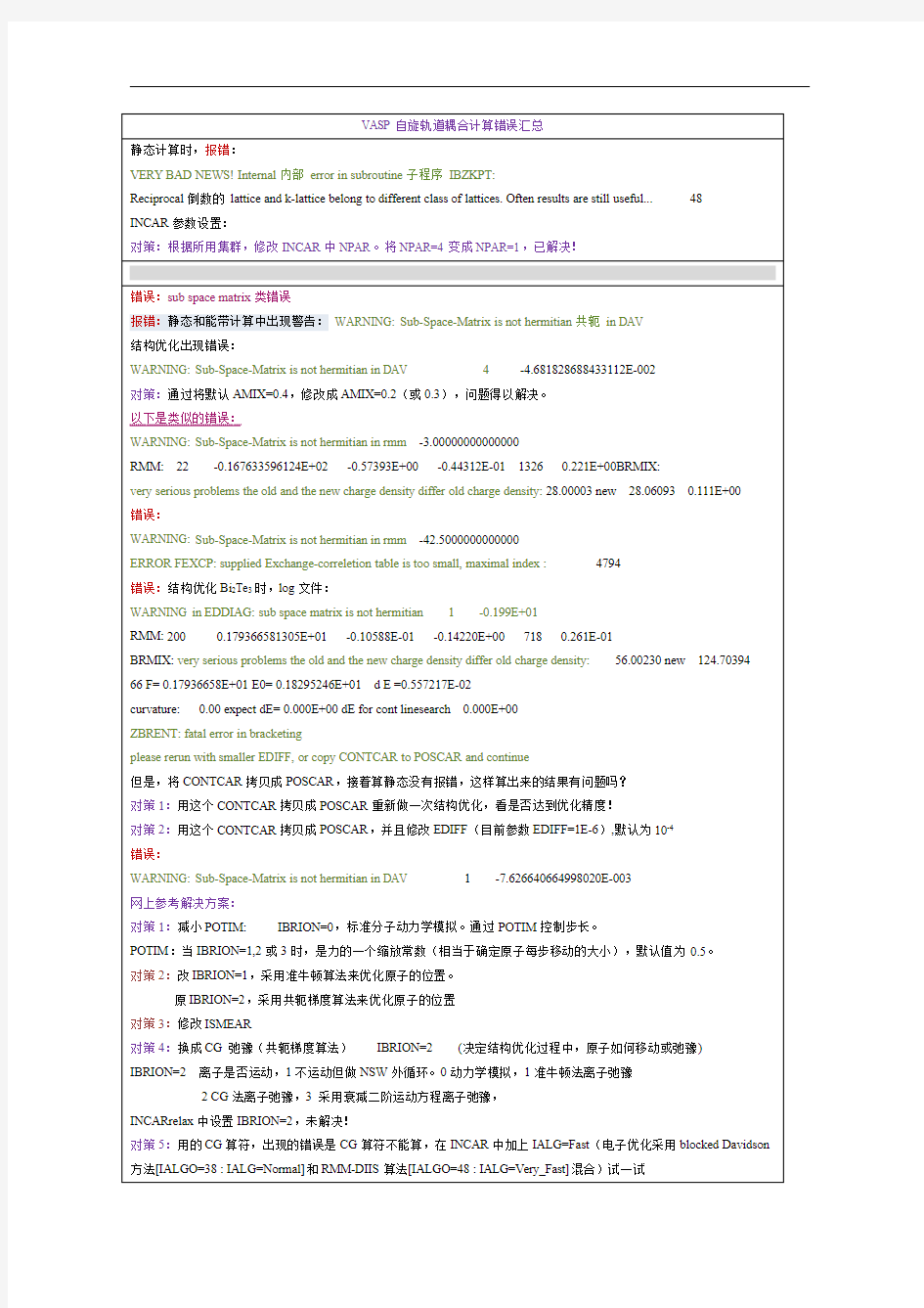
静态计算时，报错：

VERY BAD NEWS!Internal内部error in subroutine子程序IBZKPT:

Reciprocal倒数的lattice and k-lattice belong to different class of lattices.Often results are still useful (48)

INCAR参数设置：

对策：根据所用集群，修改INCAR中NPAR。将NPAR=4变成NPAR=1，已解决！

错误：sub space matrix类错误

报错：静态和能带计算中出现警告：WARNING:Sub-Space-Matrix is not hermitian共轭in DAV

结构优化出现错误：

WARNING:Sub-Space-Matrix is not hermitian in DAV4-4.681828688433112E-002

对策：通过将默认AMIX=0.4，修改成AMIX=0.2（或0.3），问题得以解决。

以下是类似的错误：

WARNING:Sub-Space-Matrix is not hermitian in rmm-3.00000000000000

RMM:22-0.167633596124E+02-0.57393E+00-0.44312E-0113260.221E+00BRMIX:

very serious problems the old and the new charge density differ old charge density:28.00003new28.060930.111E+00

错误：

WARNING:Sub-Space-Matrix is not hermitian in rmm-42.5000000000000

ERROR FEXCP:supplied Exchange-correletion table is too small,maximal index:4794

错误：结构优化Bi2Te3时，log文件：

WARNING in EDDIAG:sub space matrix is not hermitian1-0.199E+01

RMM:2000.179366581305E+01-0.10588E-01-0.14220E+007180.261E-01

BRMIX:very serious problems the old and the new charge density differ old charge density:56.00230new124.70394 66F=0.17936658E+01E0=0.18295246E+01d E=0.557217E-02

curvature:0.00expect dE=0.000E+00dE for cont linesearch0.000E+00

ZBRENT:fatal error in bracketing

please rerun with smaller EDIFF,or copy CONTCAR to POSCAR and continue

但是，将CONTCAR拷贝成POSCAR，接着算静态没有报错，这样算出来的结果有问题吗？

对策1：用这个CONTCAR拷贝成POSCAR重新做一次结构优化，看是否达到优化精度！

对策2：用这个CONTCAR拷贝成POSCAR，并且修改EDIFF（目前参数EDIFF=1E-6）,默认为10-4

错误：

WARNING:Sub-Space-Matrix is not hermitian in DAV1-7.626640664998020E-003

网上参考解决方案：

对策1：减小POTIM:IBRION=0，标准分子动力学模拟。通过POTIM控制步长。

POTIM：当IBRION=1,2或3时，是力的一个缩放常数（相当于确定原子每步移动的大小），默认值为0.5。

对策2：改IBRION=1，采用准牛顿算法来优化原子的位置。

原IBRION=2，采用共轭梯度算法来优化原子的位置

对策3：修改ISMEAR

对策4：换成CG弛豫（共轭梯度算法）IBRION=2(决定结构优化过程中，原子如何移动或弛豫)

IBRION=2离子是否运动，1不运动但做NSW外循环。0动力学模拟，1准牛顿法离子弛豫

2CG法离子弛豫，3采用衰减二阶运动方程离子弛豫，

INCARrelax中设置IBRION=2，未解决！

对策5：用的CG算符，出现的错误是CG算符不能算，在INCAR中加上IALG=Fast（电子优化采用blocked Davidson 方法[IALGO=38:IALG=Normal]和RMM-DIIS算法[IALGO=48:IALG=Very_Fast]混合）试一试

IALG=Fast(两种方法混用)

IALG=Very_Fast(等价于IALGO=48)

IALG=Normal（等价于IALGO=38）

INCAR中加上IALG=Fast已解决！（1QL、2QL已解决，3QL以上未解决）

VASP FORUM:the error is due to a LAPCK call(ZHEGV):ZHEGV computes all the eigenvalues本征值,and optionally随意地,the eigenvectors of a complex generalized Hermitian-definite eigenproblem.

there may be several reasons for that error:

1)the RMM-DIIS diagonalisation algorithm is not stable for your specific setup of the calculation.-->use ALGO=Normal (blocked Davidson)or ALGO=Fast(5steps blocked Davidson,RMM-DIIS)

用ALGO=Normal IALGO=48或者ALGO=Fast

2)

a)maybe your input geometry was not reasonable(error occurs at the very first ionic step,please have a look for the geometry data of your run in OUTCAR)or

b)the last ionic relaxation step lead to an unreasonable geometry(compare the input and output geometries of the last ionic relaxation steps in XDATCAR).

In that case(2b)it can be helpful to-->switch to a different relaxation algorithm(IBRION-tag)-->reduce the step size of the first step by setting POTIM smaller than the default value

改变IBRION，减少步长POTIM

3)The installation of the LAPACK on your machine was not done properly:use the LAPACK which is delivered with the code (vasp.4.lib/lapack_double.o)

4)If the error persist although you switched to the Davidson algorithm:on some architectures(especially SGI)some LAPACK routines are not working properly.However,it is possible to avoid the usage of the ZHEGV subroutine by commenting the line #define USE_ZHEEVX in davidson.F,subrot.F,and wavpre_noio.F and recompiling VASP.

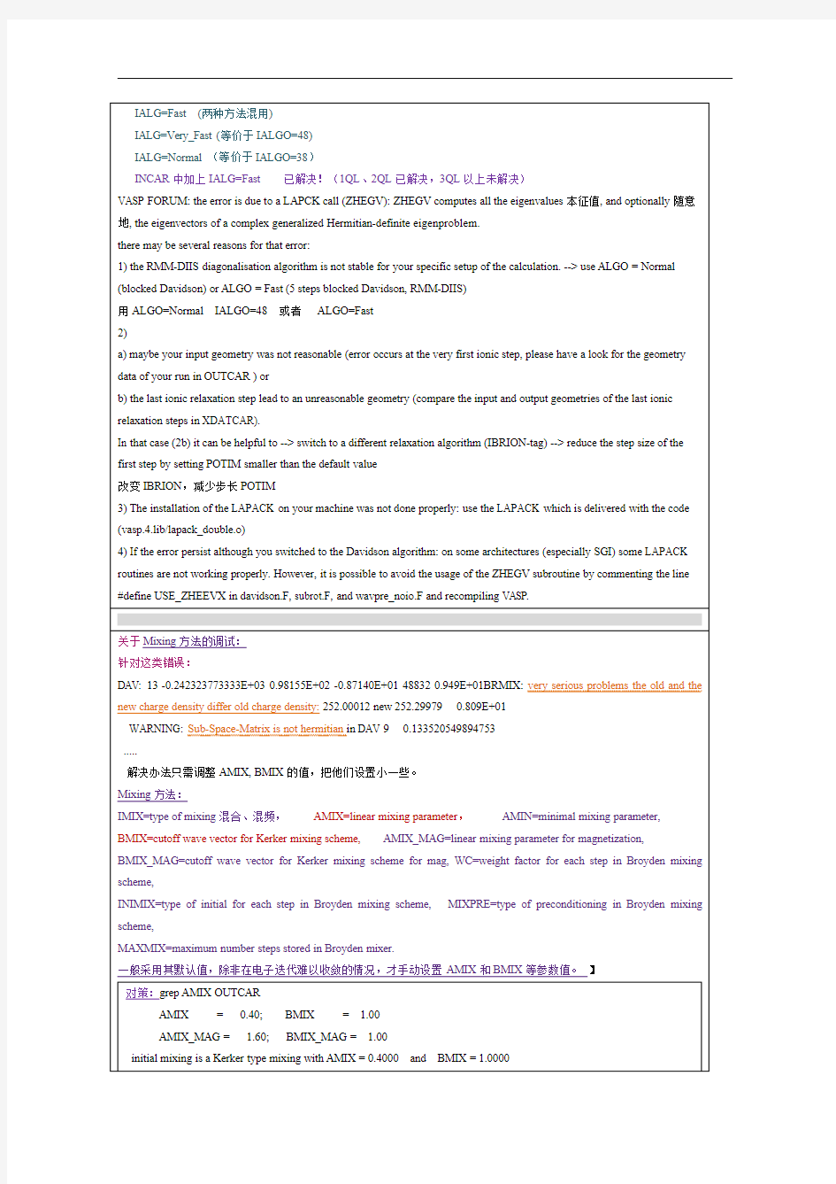
关于Mixing方法的调试：

针对这类错误：

DAV:13-0.242323773333E+030.98155E+02-0.87140E+01488320.949E+01BRMIX:very serious problems the old and the new charge density differ old charge density:252.00012new252.299790.809E+01

WARNING:Sub-Space-Matrix is not hermitian in DAV90.133520549894753

.....

解决办法只需调整AMIX,BMIX的值，把他们设置小一些。

Mixing方法：

IMIX=type of mixing混合、混频，AMIX=linear mixing parameter，AMIN=minimal mixing parameter,

BMIX=cutoff wave vector for Kerker mixing scheme,AMIX_MAG=linear mixing parameter for magnetization,

BMIX_MAG=cutoff wave vector for Kerker mixing scheme for mag,WC=weight factor for each step in Broyden mixing scheme,

INIMIX=type of initial for each step in Broyden mixing scheme,MIXPRE=type of preconditioning in Broyden mixing scheme,

MAXMIX=maximum number steps stored in Broyden mixer.

一般采用其默认值，除非在电子迭代难以收敛的情况，才手动设置AMIX和BMIX等参数值。】

对策：grep AMIX OUTCAR

AMIX=0.40;BMIX= 1.00

AMIX_MAG= 1.60;BMIX_MAG= 1.00

initial mixing is a Kerker type mixing with AMIX=0.4000and BMIX=1.0000

设置：

初始值收敛值结果

AMIX=0.0100；BMIX=0.0001AMIX=0.01;BMIX=0.00计算无误

AMIX=0.1000；BMIX=0.0010AMIX=0.10;BMIX=0.00计算无误

AMIX=0.20;BMIX=0.01AMIX=0.20;BMIX=0.01计算无误

AMIX=0.2、BMIX=0.001AMIX=0.2、BMIX=0.001计算无误

AMIX=0.3、BMIX=0.1AMIX=0.3、BMIX=0.1计算无误

AMIX=0.4AMIX=0.40;BMIX=1.00静态log:WARNING in EDDRMM:call to

ZHEGV failed,returncode=63**,能带

一样

AMIX=0.02AMIX=0.02;BMIX=1.00计算无误

AMIX=0.1AMIX=0.10;BMIX=1.00静态log:WARNING in EDDRMM:call to

ZHEGV failed,returncode=63**,能带

一样

AMIX=0.3AMIX=0.30;BMIX=1.00静态log:WARNING in EDDRMM:call to

ZHEGV failed,returncode=63**,能带

一样

BMIX=0.0001AMIX=0.40;BMIX=0.00计算无误

以上参数设置，得到的能带图都一样，如下图:

综上：设置AMIX=0.2（或0.3）,BMIX默认（省事，等于1.0），可以保证计算过程无误。还需进一步调整其他参数，算出正确的能带。

警告：算1QL弛豫、静态、能带时，都有这个提示：

ADVICE TO THIS USER RUNNING'VASP/V AMP'(HEAR YOUR MASTER'S VOICE...):You have a(more or less)

'small supercell'and for smaller cells it is recommended to use the reciprocal-space projection scheme!The real space optimization is not efficient for small cells and it is also less accurate...Therefore set LREAL=.FALSE.in the INCAR file

对策：对于较小的晶胞（原子数小于20），设置LREAL=.FALSE.，计算结果比较精确。而对于较大的晶胞，设置LREAL=Auto，这样计算速度比较快。本体系含原子5个，INCAR中LREAL=Auto。设置所有INCAR中的

LREAL=.FALSE.，重新算一遍。

对于1QL2QL3QL原子数分别为5、10、15，LREAL=.False.

对于4QL5QL6QL原子数分别为20、25、30，LREAL=Auto

自旋轨道耦合计算时，静态和能带计算中出现的错误：

ERROR:non collinear calculations require that VASP is compiled without the flag-DNGXhalf and-DNGZhalf

分析：VASP 手册中关于自旋轨道耦合计算的描述（翻译版）：

非线性计算和自旋轨道耦合：旋量是由Georg Kresse 在VASP 代码中引入的。这个代码是由David Hobbs 编写，用于处理非线性磁结构。自旋轨道耦合计算是由Olivier Lebacq and Georg Kresse 共同实现的。只有VASP4.5以上的版本才支持旋量的计算。

在INCAR 中设置LNONCOLLINEAR=.TRUE.允许执行完全非线性磁结构的计算。VASP 有能力读入之前非磁或非线性计算得到的WA VECAR 和CHGCAR 文件，然而它不可能扭转局域在指定原子处的磁场。因此在实际操作中，我们推荐分两步执行非线性计算：

第一步，计算计算非磁性基态，产生WA VECAR 和CHGCAR 文件。

第二步，读入WA VECAR 和CHGCAR 文件，通过设置MAGMOM 参数，提供初始的磁矩。对于非线性设置，在MAGMOM 这一行，每个离子必须设置三个值。这三项分别对应每个离子在x,y,z 方向的初始局域磁矩值。MAGMOM =100

010

这一行，给第一个原子赋予的初始磁矩值沿x 方向，第二个原子的初始磁矩值沿y 方向。

注意：只有在ICHARG=2（即不读入之前CHGCAR 的情况）或者CHGCAR 文件中只包含电荷但是不包括磁密度数据的情况（即之前那一步进行了非磁的计算）下，才需要通过MAGMOM 设定初始磁矩值。LSORBIT-tag

Supported as of VASP.4.5.

【设置LSORBIT=.TRUE.表示计算自旋轨道耦合，并附带自动设置了LNONCOLLINEAR=.TRUE.】

LSORBIT=.TRUE.只能用于PAW 赝势，不能用于超软赝势。如果不考虑自选轨道耦合，则能量不依赖磁矩的方向，也就是说，旋转所有的磁矩以同一个角度，让它们拥有相等的能量。不考虑自选轨道耦合的时候，不需要定义自旋量子化坐标。开启自旋轨道耦合设置以下参数：LSORBIT =.TRUE.

SAXIS =s_x s_y s_z (自旋量子化轴，默认值SAXIS=(0+,0,1))GGA_COMPAT =.FALSE.!应用球面截断能到梯度场

其中SAXIS 默认=(0+,0,1)（0+表示沿x 轴方向一个无穷小的正数）。当需要计算亚meV 能量尺度的微小能量差异（一般指磁各向异性计算的情况）时，需要设置GGA_COMPAT 这个参数。现在所有关于坐标轴(Sx,Sy,Sz)的磁矩都给出来了，我们采用VASP 中给出关于这个坐标轴所有磁矩和自旋状量子读写惯例。

这包括INCAR 文件中的MAGMOM 行，OUTCAR 和PROCAR 文件中的总和局域磁矩，WA VECAR 文件中的类自旋轨道，CHGCAR 文件中的磁密度。笛卡尔坐标系中的磁分量由以下等式得到：

axis

z axis x z axis z axis y x y axis z axis y axis x x m m m m m m m m m m m )cos()sin()sin()sin()cos()sin()cos()cos(*)sin()sin()cos()cos(ββαβααβαβααβ+-=++=+-=其中，maxis 是外部可见的磁矩值，此处的α是SAXIS 矢量(sx,sy,sz)和笛卡尔坐标x 轴的夹角，β是SAXIS 矢量和笛卡

尔坐标z 轴的夹角,

z

y x x

y s s s a s s a |

|tan

,tan

2

2+==βα,以下等式得到逆变化：

z y x axis y x axis z

y x axis m m m m m m m m m m m z

y

x )cos()sin()sin()cos()sin()cos()sin()sin()sin()cos()cos()cos(βαβαβααβαβαβ++=+-=++=不难看出，默认值(sx,sy,sz)=(0+,0,1)，两个角度都是0，即β=0和α=0。在这种情况下，内部转换简单地等于外部地转换：

axis

z z axis

y y axis x x m m m m m m ===,,，第二种重要的情况，是

0=axis x m 和0=axis

y

m ，在这种情况下：

2

222

22/)(cos /)cos(*)sin(z y x z axis z axis x z y z

y z axis z axis z x s s s s m m m m s s s s m m m x ++===

++==βαβ

因此现在磁矩是平行于SAXIS矢量。这样有两种方式去旋转自旋到任意方向，即通过改变初始的磁矩MAGMOM或改变SAXIS。为了给计算赋予平行于一个选定的矢量(x,y,z)的初始磁矩，可以通过设定（假定是单原子原胞）：MAGMOM=x y z!局域磁矩x y z

SAXIS=001!量子轴平行于z轴

或者

MAGMOM=00total_magnetic_moment!局域磁矩平行于SAXIS

SAXIS=x y z!量子轴平行于矢量(x,y,z)

两种设置都必须在相同能量的标准/辐射（原则、根源）场，但是要实现第二种方法，通常更加精确。第二种方法，也允许读入之前存在的WA VECAR文件（由线性计算还是非线性计算产生的都可以），然后继续用一个不同的自旋方向计算。当读入一个非线性WA VECAR文件，自旋假定平行于SAXIS（因此VASP将仅仅输出一个z轴方向的磁矩）。推荐计算磁各项异性的步骤如下：

先做线性计算，得到一个WA VECAR和CHGCAR文件。

加入以下参数：

LSORBIT=.TRUE.

ICHARG=11!非自洽计算,读入CHGCAR

LMAXMIX=4!对于d电子元素设置LMAXMIX=4,f电子元素设置LMAXMIX=6

!在线性计算中，需要设置LMAXMIX

SAXIS=x y z!磁场的方向

NBANDS=2*线性计算能带数

GGA_COMPAT=.FALSE.!在梯度场中应用球面截断能

VASP读入WA VECAR和CHGCAR文件，将自旋量子轴对齐SAXIS矢量，这意味着现在磁场平行于SAXIS矢量，执行非线性计算。通过比较不同方向的能量，可以确定磁各向异性。请记住，原则上，在VASP中一个完全地自洽计算(ICHARG=1)也是有可能的，但是这种情况将会允许自旋波函数从它们的初始值旋转到平行于SAXIS矢量，直到获得正确的基态，也就是，直到磁矩平行于易磁化轴。实际操作中，这种旋转非常缓慢，直到自旋获得少量能量重新定位。因此，如果收敛标准太精确，完全地自洽计算可以得到一个比较合理的结果（我们实验过的几种自洽计算都没有问题。）要非常小心对称性。我们建议选择计算自旋轨道耦合时，完全关掉对称性(ISYM=0)。通常会从一个自旋方向到另一个自旋方向k点的设置会发生改变，进而恶化转换的结果（如果k点改变WA VECAR将不会被正确地重新读取）。GGA_COMPAT通常需要，应该被设置，因为磁各向异性能量通常需要精确到亚meV数量级。

当计算自旋轨道耦合，特别是磁各向异性时通常需要非常小心：能量差异非常小，k点的收敛冗长而且缓慢，需要耗费大量的计算时间。此外，这一特征--尽管长期存在于VASP中--在最新的版本中依然存在，你可以尝试频繁地升级发现这一点。不敢保证，你的结果是有用的！此处根据README文件做了一个小小的总结：

20.11.2003:提出的GGA程序轻微的破坏了非正交体系晶胞的对称型。球面截断能应用于梯度及互逆空间中的所有中间结果。GGA引起的轻微的改变（通常每个原子0.1meV），却对磁各项异性很重要。

05.12.2003:继续...现在VASP.4.6默认旧的行为GGA_COMPA T=.TRUE.，新的行为将可以通过在INACR中设置GGA_COMPAT=.FALSE.得到。

12.08.2003:主要的错误出现在symmetry.F和paw.F：非线性计算的对称性例程没有正确的执行。

如果你阅读了以上内容，就会意识到在VASP.4.6和VASP.5.2版本中进行非线性计算推荐设置GGA_COMPAT=.FALSE.，这样可以提升GGA计算的数值精度。

VASP:Non-collinear calculations and spin orbit coupling:Spinors旋量were included by Georg Kresse in the VASP code.The code required for the treatment处理of non-collinear magnetic structures was written by David Hobbs,and spin-orbit coupling was implemented实施、执行by Olivier Lebacq and Georg Kresse.Spinors are only supported as of VASP.4.5. Subsections：分段、子章节、下一级栏目

LNONCOLLINEAR-tag

Supported支持as of VASP.4.5.

Setting LNONCOLLINEAR=.TRUE.in the INCAR file allows to perform fully non-collinear magnetic structure calculations.VASP is capable 有能力的of reading WAVECAR and CHGCAR files from previous 之前的non-magnetic 非磁or collinear 线性calculations,it is however not possible to rotate 旋转、转动the magnetic field locally on selected atoms.Hence 因此,in practice 在实践中,we recommend 推荐to perform non-collinear calculations in two steps:First,calculate the non magnetic groundstate 基态and generate a WA VECAR and CHGCAR file.

Second,read the WA VECAR and CHGCAR file,and supply 提供initial magnetic moments by means of the MAGMOM tag (compare Sec.6.13).For a non-collinear setup,three values must be supplied for each ion in the MAGMOM line.The three entries correspond to the initial local magnetic moment for each ion in x,y and z direction respectively.The line MAGMOM =100

010

Initialises 赋初值the magnetic moment on the first atom in the x-direction,and on the second atom in the y direction.Mind,that the MAGMOM line supplies initial magnetic moments only if ICHARG=2,or if the CHGCAR file contains only charge but no magnetisation density.

LSORBIT=.TRUE.Switches 接通、开启on spin-orbit coupling and automatically sets LNONCOLLINEAR=.TRUE..This option 选项、选择works only for PAW potentials and is not supported for ultrasoft pseudopotentials.If spin-orbit coupling is not included,the energy does not depend on 依赖the direction of the magnetic moment,i.e.也就是说rotating 旋转all magnetic moments 磁矩by the same angle results exactly in the same energy.Hence 因此there is no need to define the spin quantization axis 自旋量子化坐标轴,as long as 只要spin-orbit coupling is not included.Spin-orbit coupling,however,couples 一对、一双the spin to the crystal structure.Spin orbit coupling is switched on 开启by selecting LSORBIT =.TRUE.

SAXIS =s_x s_y s_z (quantisation axis for spin 自旋量子化轴)

GGA_COMPAT =.FALSE.!apply spherical 球面cutoff 截断能on gradient field 梯度场

where the default for SAXIS=(0+,0,1)(the notation 符号0+implies 意味着an infinitesimal 无穷小small positive number in

x

?direction).The flag GGA_COMPAT (see Sec.6.42)is optional 选项and should be set when small energy differences in the sub 副、下标meV regime 体制、状态need to be calculated (often the case for magnetic anisotropy calculations 磁各向异性计算).All magnetic moments are now given with respect to 关于the axis 坐标轴(S x ,S y ,S z ),where we have adopted 应用the convention 惯例that all magnetic moments and spinor-like quantities written or read by VASP are given with respect to this axis .

This includes the MAGMOM line in the INCAR file,the total and local magnetizations in the OUTCAR and PROCAR file,the spinor 自旋量-like orbitals in the WAVECAR file,and the magnetization density in the CHGCAR file.With respect to the cartesian 笛卡尔lattice vectors the components 组件、部分of the magnetization are (internally 内部地、内在的)given by

axis z

axis x z axis z axis y x y axis z axis y axis x x m m m m m m m m m m m )cos()sin()sin()sin()cos()sin()cos()cos(*)sin()sin()cos()cos(ββαβααβαβααβ+-=++=+-=Where m axis is the externally 外部地visible 可得到的，现有的，可见的magnetic moment.Here,αis the angle between the SAXIS vector (s x ,s y ,s z )and the cartesian vector

x

?,and βis the angle between the vector SAXIS and the cartesian vector z ?:z

y x x

y s s s a s s a |

|tan

,tan

2

2+==βαThe inverse 倒转、翻转transformation 转化、转换is given by

z y x axis y x axis z

y x axis m m m m m m m m m m m z

y

x )cos()sin()sin()cos()sin()cos()sin()sin()sin()cos()cos()cos(βαβαβααβαβαβ++=+-=++=It is easy to see that for the default (s x ,s y ,s z )=(0+,0,1),both angles are zero,i.e.β=0and α=0.In this case,the internal representation is simply equivalent to the external representation:axis

z z axis

y y axis x x m m m m m m ===,,The second important case,is 0=axis x m and 0=axis y

m .In this case

2

222

22/)(cos /)cos(*)sin(z y x z axis z axis x z y z

y z axis z axis z x s s s s m m m m s s s s m m m x ++===

++==βαβHence 因此、今后now the magnetic moment is parallel to the vector SAXIS.Thus there are two ways to rotate the spins in an arbitrary 任意的direction,either by changing the initial magnetic moments MAGMOM or by changing SAXIS.

To initialise calculations with the magnetic moment parallel to a chosen vector (x,y,z),it is therefore 因此possible to either specify 指定(assuming 假定、假设a single atom in the cell)MAGMOM =x y z !local magnetic moment in x,y,z SAXIS =001!quantisation axis parallel to z

or

MAGMOM =00total_magnetic_moment !local magnetic moment parallel to SAXIS

SAXIS =x y z

!quantisation axis parallel to vector (x,y,z)

Both setups should in principle yield exactly the same energy,but for implementation 实现reasons the second method is usually more precise 精确.The second method also allows to read a preexisting WAVECAR file (from a collinear or non collinear run),and to continue the calculation with a different spin orientation.When a non collinear WAVECAR file is read,the spin is assumed 假定to be parallel to SAXIS (hence 因此VASP will initially report a magnetic moment in the z-direction only).The recommended 被推荐的procedure 过程、步骤for the calculation of magnetic anisotropies is therefore 因而、表示结果(please check the section on LMAXMIX 6.63):

?Start with a collinear calculation and calculate a WA VECAR and CHGCAR file.?

Add the tags

LSORBIT =.TRUE.ICHARG =11!non selfconsistent run,read CHGCAR

LMAXMIX =4

!for d elements increase LMAXMIX to 4,f:LMAXMIX =6

!you need to set LMAXMIX already in the collinear calculation SAXIS =x y z

!direction of the magnetic field

NBANDS =2*number of bands of collinear run

GGA_COMPAT =.FALSE.!apply spherical cutoff on gradient field

VASP reads in the WA VECAR and CHGCAR files,aligns 排列the spin quantization axis parallel to SAXIS,which implies 意味着that the magnetic field is now parallel to SAXIS,and performs a non selfconsistent calculation.By comparing the energies for different orientations the magnetic anisotropy can be determined 确定.Please mind,that a completely selfconsistent calculation (ICHARG=1)is in principle 大体上、原则上also possible with VASP,but this would allow the the spinor wavefunctions to rotate from their initial orientation parallel to SAXIS until the correct groundstate is obtained,i.e.until the magnetic moment is parallel to the easy axis （?=the easy magnetic axis ）.In practice this rotation will be slow,since reorientation 再定位of the spin gains 获得little energy.Therefore if the convergence 收敛criterion 标准is not too tight,sensible 明智的results might be obtained even for fully selfconsistent calculations (in the few cases we have tried 可靠地，试验过的selfconsistentcy worked without problems).

Be very careful with symmetry.We recommend 建议to switch off 关掉symmetry (ISYM=0)altogether 完全地,when spin orbit coupling is selected.Often the k-point set changes from one to the other spin orientation,worsening 恶化the transferability of the results (also the WA VECAR file can not be reread properly 正确地if the number of k-points changes).The flag GGA_COMPAT is usually required and should be set,since magnetic anisotropy energies are often in the sub meV regime (see Sec.6.42).

Generally be extremely 非常careful,when using spin orbit coupling and,specifically 特别地,magnetic anisotropies:energy differences are tiny 微小的,k-point convergence 收敛is tedious 冗长乏味and slow,and the computer time might be huge.

Additionally此外,this feature这一特征--although long implemented应用in VASP--is still in a late beta stage,as you might deduce from推断，从...得出结论the frequent频繁的updates升级、更新.No promise允诺,that your results will be useful! Here is a small summary总结from the README file:

20.11.2003:The present提出GGA routine程序breaks the symmetry slightly轻微地for non orthorhombic正交晶系cells.A spherical球面的cutoff is now imposed on应用于the gradients and all intermediate中间的results in reciprocal互逆space.This changes the GGA results slightly(usually by0.1meV per atom),but is important for magnetic anisotropies.

05.12.2003:continue...Now VASP.4.6defaults to the old behavior GGA_COMPAT=.TRUE.,the new behavior can be obtained by setting GGA_COMPAT=.FALSE.in the INCAR file.

12.08.2003:MAJOR主要的BUG故障FIX固定in symmetry.F and paw.F:for non-collinear calculations the symmetry routines惯例did not work properly正确地

If you have read the previous lines,you will realize that it is recommended推荐to set GGA_COMPA T=.FALSE.for non collinear calculations in VASP.4.6and VASP.5.2,since this improves the numerical precision of GGA calculations.

degree:

BSc：Bachelor of Science理科学士MD MS：master硕士PhD：Doctor of Philosophy博士学位

AA Associate degree of Arts大专文科学位AAS Associate degree of Arts and Science大专文理科学位

AS Associate degree of Science大专理科学位BA Bachelor of Arts文科本科学位

BS Bachelor of Science理科本科学位MA Master of Arts文科硕士

MBA Master of Business Administration商学硕士MS Master of Science理科硕士

Ph.D.Doctor of Phiolosphy哲学(通才)博士JD Doctor of Journalism新闻博士

MD Doctor of Medicine医学博士DVM Doctor of Veterinry兽医博士

Call to ZHEGV failed

Error EDDDAV:Call to ZHEGV failed.Returncode=1318

The earlier solution suggested by admin（DOS操作系统中，超级管理员。行政、管理）(suppressing制止的the line#define USE_ZHEEVX in davidson.F,subrot.F,and wavpre_noio.F and recompiling VASP)does not work,i.e.the same error messages, and the same indication迹象、表示of ZHEGV failure,still appear出现.I may add now that the problem appears both with the lapack which comes with VASP and with a system-native lapack library.The warnings given suggest that the problem actually appears at an earlier stage阶段,in which a matrix is generated with inadequate不适当的values which make it nonhermitian, and consequently ZHEGV fails even if working correctly;the solution thus would not be to avoid using ZHEGV,but to avoid an incorrect generation of the said matrix.Can someone give an idea to really solve the problem?

答：Please try if it works by adding"LSCALAPACK=.FALSE."in your INCAR.

对策：grep LSCALAPACK OUTCAR空

设置：LSCALAPACK=.FALSE

问：No;adding"LSCALAPACK=.FALSE."in INCAR makes no dfference,the problem continues the same.

问：I was successful to fix this problem解决此问题by using IALGO=48instead of IALGO=Default。

unfortunately,when i set IALGO=48,the new warning is：

WARNING in EDDRMM:call to ZHEGV failed,returncode=6314

how to solve this problem?what does"ZBRENT"mean?

对策：grep IALGO OUTCAR

IALGO=68algorithm（INCAR ALGO=Fast）

设置：IALGO=48

please try one of the following:

1)choose a different algorithm for ionic optimization(IBRION=1)采用准牛顿算法来优化原子位置

2)set ADDGRID=.True.in INCAR(only for vasp releases发布管理、释放、豁免4.4.5and newer)

对策：grep ADDGRID OUTCAR空

grep IBRION OUTCAR

IBRION=2ionic relax:0-MD1-quasi-New2-CG

设置ADDGRID=.True.In INCAR

设置IBRION=1in INCAR

错误：

internal ERROR RSPHER:running out of buffer00

1310

nonlr.F:Out of buffer RSPHER

得到的CONTCAR是空的！

结构优化出现错误：

Internal内部的、内在的ERROR RSPHER:running out of buffer缓冲00

1310

nonlr.F:Out of buffer RSPHER

解决：将NPAR=1修改成4（或者2），问题得以解决。

分两步（scf非磁线性计算，bands读取CHGCAR、WAVECAR做非线性自旋轨道耦合计算），能带计算出错：ERROR:while reading WAVECAR,plane wave coefficients系数changed5728628837

Solution:You have to continue with the converged收敛CHGCAR,because most probably,you will increase增加/change改变the k-mesh to get a denser密集的、浓厚的k-grid to calculate the DOS accurately.Then,WAVECAR will not be read correctly because the wavefunction-coefficients波函数-系数are stored存储k-point wise明智的concerning涉及the READ error of CHGCAR:please check whether the FFT meshes have changed.please make sure that

1)the CHGCAR really is in the working directory目录at runtime运行时间

2)the fft meshes of CHGCAR are compatible兼容的

The main points is in this sentence"plane wave coefficients changed",I think the ISMEAR you used in scf and noscf process is different,therefore,the plane wave coefficients changed in these two process is not identical完全相同的.You can find the values of NGXF,NGYF and NGZF in the CHGCAR or OUTCAR of the scf,and then add these three parameters in the INCAR of the nonscf.OK,the problem is resolved.

在静态计算的CHGCAR或者OUTCAR中找到NGXF,NGYF和NGZF，将这些参数加到非静态计算的INCAR中：grep NGXF OUTCAR

dimension x,y,z NGXF=64NGYF=64NGZF=840

support grid NGXF=64NGYF=64NGZF=840

NGXF,Y,Z is equivalent to a cutoff of25.43,25.43,25.05a.u.

对策：在能带计算INCAR中加入NGXF=64NGYF=64NGZF=840

修改之后，bands中出现错误：

ERROR:non collinear calculations require that VASP is compiled without the flag-DNGXhalf and-DNGZhalf

解决：待解决!

网上经验：

non collinear calculations require that VASP is compiled without the flag-DNGXhalf and-DNGZhalf.

一、请加入SOC

1）INCAR中加入

LNONCOLLINEAR=.True.

LSORBIT=.True.

LORBMOM=.True.

ISYM=-1（？不对，ISYM取值0,1,2,3）

【SAXIS=自旋轴方向；MAGMOM=每个原子的初始磁矩值】

2)不要忘记

to include SOC,please

1)add the following lines to INCAR

LNONCOLLINEAR=.True.

LSORBIT=.True.

SAXIS=#please give the spin quantization axis here,like001for the z-axis)

MAGMOM=#please give a triplet of numbers for each atom here,and please have a look at the manual(chapter non-collinear calculations and spin-orbit tag)on how the direction of the magnetic moments has to be defined with respect to the spin-quantization axis)

LORBMOM=.True.

ISYM=-1

2）不要忘记如果你用的vasp不包含任何预编译程序命令-DNGXhalf,-DNGZhalf,-DwNGXhalf,-DwNGZhalf，你必须重新编译vasp，因为这些参数通常对于非线性磁性计算是必要的，在DOSCAR中的第二块数据包含了E和4列s,p,d，如下：rho,m_x,m_y,m_z，

2)don't forget that you may have to re-compile vasp without any of the precompiler(CPP)flags set:-DNGXhalf,-DNGZhalf, -DwNGXhalf,-DwNGZhalf,as necessary for non-collinear runs in general for non-collinear magnetism,the second block of data in DOSCAR contains E,and4columns for each,s,p,d,giving:

rho,m_x,m_y,m_z

with m....magnetisation，it makes absolutely NO SENSE to set ISPIN=2(up and down)for non-clollinear runs,therfore this tag is ignored when it s read from INCAR.

Symbol Description

ΓCenter of the Brillouin zone

Simple cube

M Center of an edge

R Corner point

X Center of a face

Face-centered cubic

K Middle of an edge joining two hexagonal faces

L Center of a hexagonal face

U Middle of an edge joining a hexagonal and a square face

W Corner point

X Center of a square face

Body-centered cubic

H Corner point joining four edges

N Center of a face

P Corner point joining three edges

Hexagonal

A Center of a hexagonal face

H Corner point

K Middle of an edge joining two rectangular faces

L Middle of an edge joining a hexagonal and a rectangular face

M Center of a rectangular face

1)it does not look to me as if the magnetic convergence is particularly bad.(please dont compare the moments stemming from

the augmentation to the total moments).

have you decreased AMIX,BMIX,AMIX_MAG and BMIX_MAG for this run?

2)the mixing parameters must not have any influence on the converged total energies.

3)if your system has a magnetic moment,you have to set ISPIN.

unless you set LNONCOLLINEAR explicitely,collinear magnetism is assumed by default,there is nothing to be specified in extra(except from starting with FM or AFM configuration by choosing the MAGMOMs accordingly)

4)please in any case check if the convergence of ALL ionic steps is bad.(consider that it may be possible that you relaxed into an unreasonable geometry which does not converge electronically).

without knowing further details,I would recommend to try the following:

please keep the low mixing parameters check if the k-mesh is converged try if a different BZ-integration(ISMEAR=1)and slightly larger smearing(SIGMA)helps set LMAXMIX=6if your system contains d-elements

ISYM-tag and SYMPREC-tag

ISYM=0|1|2|3

Default1

switch symmetry on(1,2or3)or off(0).

For ISYM=2a more efficient,memory conserving symmetrisation of the charge density is used.This reduces memory requirements in particular for the parallel version.ISYM=2is the default if PAW data sets are used.

ISYM=1is the default if VASP runs with US-PP’s.

For ISYM=3,the forces and the stress tensor only are symmetrized,whereas the charge density is left unsymmetrized (VASP.5.1only).

This option might be useful in special cases,where charge/orbital ordering lowers the crystal symmetry,and the user wants to conserve【保存,保藏】the symmetry of the positions during relaxation.

However,the flag must be used with great caution,since a lower symmetry due to charge/orbital ordering,in principle also requires to sample the Brillouin zone using

a k-point mesh compatible with the lower symmetry caused by charge/orbital ordering.

The program determines automatically the point group symmetry and the space group according to the POSCAR file and the line MAGMOM in the INCAR file.

The SYMPREC-tag(VASP.4.4.4and newer versions only)determines how accurate the positions in the POSCAR file must be.The default is10?5,which is usually suffiently large even if the POSCAR file has been generated with a single precision

program.

Increasing the SYMPREC tag means,that the positions in the POSCAR file can be less accurate.

During the symmetry analysis,VASP determines

?the Bravais lattice type of the supercell,

?the point group symmetry and the space group of the supercell with basis(static and dynamic)-and prints the names

of the group(space group:only’family’),

?the type of the generating elementary(primitive)cell if the supercell is a non-primitive cell,

?all’trivial non-trivial’translations(=trivial translations of the generating elementary cell within the supercell)—needed for symmetrisation of the charge,

?the symmetry-irreducible set of k-points if automatic k-mesh generation was used

and additionally the symmetry irreducible set of tetrahedra if the tetrahedron method was chosen together with the automatic k-mesh generation and of course also the corresponding weights(’symmetry degeneracy’),

?and tables marking and connecting symmetry equivalent ions.The symmetry analyses is done in four steps:

?First the point group symmetry of the lattice(as supplied by the user)is determined.

?Then tests are performed,whether the basis breaks symmetry.Accordingly these symmetry operations are removed.

?The initial velocities are checked for symmetry breaking.

?Finally,it is checked wheter MAGMOM breaks the symmetry.Correspondingly themagnetic symmetry group is determined (VASP.4.4.4and newer releases only;if you use older version please also see section6.12).The program symmetrises automatically:

?The total charge density according to the determined space group

?The forces on the ions according to the determined space group.

?The stress tensor according to the determined space group

Why is symmetrisation necessary:Within LDA the symmetry of the supercell and the charge density are always the same.

This symmetry is broken,because a symmetry-irreducible set of k-points is used for the calculation.

To restore the correct charge density and the correct forces it is necessary to symmetrise these quantities.

It must be stressed that VASP does not determine the symmetry elements of the primitive cell.If the supercell has a lower symmetry than the primitive cell only the lower symmetry of the supercell is used in the calculation.In this case one should

not expect that forces that should be zero according to symmetry will be precisely zero in actual calculations.

The symmetry of the primitive cell is in fact broken in several places in VASP:

?local potential:

In reciprocal space,the potential V(G)should be zero,if G is not a reciprocal lattice vector of the primitive cell.

For PREC=Med,this is not guaranteed due to”aliasing”or wrap around and the charge density(and therefore the Hatree potential)might violate this point.But even for PREC=High,small errors are introduced,because the exchange correlation potential Vxc is calculated in real space.

?k-points:

In most cases,the automatic k-point grid does not have the symmetry of the primitive cell.

错误：

internal ERROR:DEPLE:IRDMAX must be increased to0

internal ERROR:DEPLE:IRDMAX must be increased to0

错误：

ERROR FEXCF:supplied exchange-correlation table is too small,maximal index:9344428

计算soc能带时，选择ISTART=1，即读入静态计算得到的WA VECAR

能带计算出错：

ERROR:while reading WA VECAR,plane wave coefficients changed16135