Matlab偏微分方程求解方法

Matlab 偏微分方程求解方法

目录：

§1 Function Summary on page 10-87

§2 Initial Value Problems on page 10-88

§3 PDE Solver on page 10-89

§4 Integrator Options on page 10-92

§5 Examples” on page 10-93

§1 Function Summary

1.1 PDE Solver” on page 10-87

1,2 PDE Helper Functi on” on page 10-87

1.3 PDE Solver

This is the MATLAB PDE solver.

PDE Helper Function

§2 Initial Value Problems

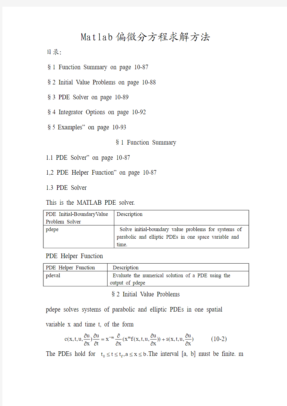
pdepe solves systems of parabolic and elliptic PDEs in one spatial variable x and time t, of the form

)x

u ,u ,t ,x (s ))x u ,u ,t ,x (f x (x x t u )x u ,u ,t ,x (c m m ??+????=????- (10-2) The PDEs hold for b x a ,t t t f 0≤≤≤≤.The interval [a, b] must be finite. m

can be 0, 1, or 2, corresponding to slab, cylindrical, or spherical symmetry,respectively. If m > 0, thena ≥0 must also hold.

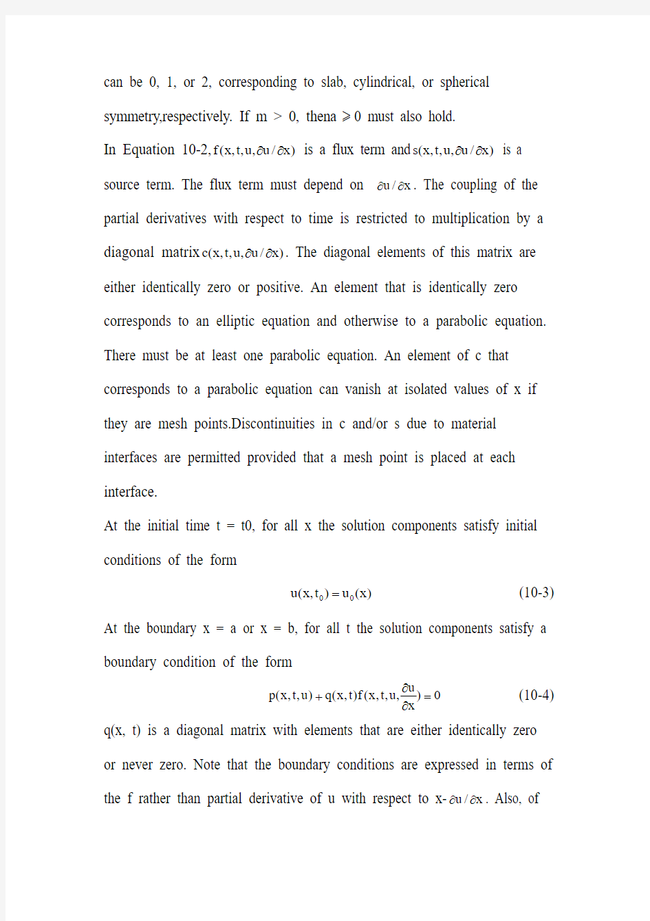
In Equation 10-2,)x /u ,u ,t ,x (f ?? is a flux term and )x /u ,u ,t ,x (s ?? is a source term. The flux term must depend on x /u ??. The coupling of the partial derivatives with respect to time is restricted to multiplication by a diagonal matrix )x /u ,u ,t ,x (c ??. The diagonal elements of this matrix are either identically zero or positive. An element that is identically zero corresponds to an elliptic equation and otherwise to a parabolic equation. There must be at least one parabolic equation. An element of c that corresponds to a parabolic equation can vanish at isolated values of x if they are mesh points.Discontinuities in c and/or s due to material interfaces are permitted provided that a mesh point is placed at each interface.

At the initial time t = t0, for all x the solution components satisfy initial conditions of the form

)x (u )t ,x (u 00= (10-3)

At the boundary x = a or x = b, for all t the solution components satisfy a boundary condition of the form

0)x

u ,u ,t ,x (f )t ,x (q )u ,t ,x (p =??+ (10-4) q(x, t) is a diagonal matrix with elements that are either identically zero or never zero. Note that the boundary conditions are expressed in terms of the f rather than partial derivative of u with respect to x-x /u ??. Also, of

the two coefficients, only p can depend on u.

§3 PDE Solver

3.1 The PDE Solver

The MATLAB PDE solver, pdepe, solves initial-boundary value problems for systems of parabolic and elliptic PDEs in the one space variable x and time t.There must be at least one parabolic equation in the system.

The pdepe solver converts the PDEs to ODEs using a second-order accurate spatial discretization based on a fixed set of user-specified nodes. The discretization method is described in [9]. The time integration is done with ode15s. The pdepe solver exploits the capabilities of ode15s for solving the differential-algebraic equations that arise when Equation 10-2 contains elliptic equations, and for handling Jacobians with a specified sparsity pattern. ode15s changes both the time step and the formula dynamically.

After discretization, elliptic equations give rise to algebraic equations. If the elements of the initial conditions vector that correspond to elliptic equations are not “consistent” with the discretization, pdepe tries to adjust them before eginning the time integration. For this reason, the solution returned for the initial time may have a discretization error comparable to that at any other time. If the mesh is sufficiently fine, pdepe can find consistent initial conditions close to the given ones. If pdepe displays a

message that it has difficulty finding consistent initial conditions, try refining the mesh. No adjustment is necessary for elements of the initial conditions vector that correspond to parabolic equations.

PDE Solver Syntax

The basic syntax of the solver is:

sol = pdepe(m,pdefun,icfun,bcfun,xmesh,tspan)

Note Correspondences given are to terms used in “Initial Value Problems” on page 10-88.

The input arguments are

m: Specifies the symmetry of the problem. m can be 0 =slab, 1 = cylindrical, or 2 = spherical. It corresponds to m in Equation 10-2. pdefun: Function that defines the components of the PDE. It

computes the terms f,c and s in Equation 10-2, and has the form

[c,f,s] = pdefun(x,t,u,dudx)

where x and t are scalars, and u and dudx are vectors that approximate the solution and its partial derivative with respect to . c, f, and s are column vectors. c stores the diagonal elements of the matrix .

icfun: Function that evaluates the initial conditions. It has the form

u = icfun(x)

When called with an argument x, icfun evaluates and returns the initial values of the solution components at x in the column vector u.

bcfun:Function that evaluates the terms and of the boundary conditions. It

has the form

[pl,ql,pr,qr] = bcfun(xl,ul,xr,ur,t)

where ul is the approximate solution at the left boundary xl = a and ur is the approximate solution at the right boundary xr = b. pl and ql are column vectors corresponding to p and the diagonal of q evaluated at xl. Similarly, pr and qr correspond to xr. When m>0 and a = 0, boundedness of the solution near x = 0 requires that the f vanish at a = 0. pdepe imposes this boundary condition automatically and it ignores values returned in pl and ql.

xmesh:Vector [x0, x1, ..., xn] specifying the points at which a numerical solution is requested for every value in tspan. x0 and xn correspond to a and b , respectively. Second-order approximation to the solution is made on the mesh specified in xmesh. Generally, it is best to use closely spaced mesh points where the solution changes rapidly. pdepe does not select the mesh in automatically. You must provide an appropriate fixed mesh in xmesh. The cost depends strongly on the length of xmesh. When , it is not necessary to use a fine mesh near to x=0 account for the coordinate singularity.

The elements of xmesh must satisfy x0 < x1 < ... < xn.

The length of xmesh must be ≥3.

tspan:Vector [t0, t1, ..., tf] specifying the points at which a solution is requested for every value in xmesh. t0 and tf correspond to

t and f t,

respectively.

pdepe performs the time integration with an ODE solver that selects both the time step and formula dynamically. The solutions at the points specified in tspan are obtained using the natural continuous extension of the integration formulas. The elements of tspan merely specify where you want answers and the cost depends weakly on the length of tspan.

The elements of tspan must satisfy t0 < t1 < ... < tf.

The length of tspan must be ≥3.

The output argument sol is a three-dimensional array, such that

?sol(:,:,k) approximates component k of the solution .

?sol(i,:,k) approximates component k of the solution at time tspan(i) and mesh points xmesh(:).

?sol(i,j,k) approximates component k of the solution at time tspan(i) and the mesh point xmesh(j).

4.2 PDE Solver Options

For more advanced applications, you can also specify as input arguments solver options and additional parameters that are passed to the PDE functions.

options:Structure of optional parameters that change the default integration properties. This is the seventh input argument.

sol = pdepe(m,pdefun,icfun,bcfun,xmesh,tspan,options)

See “Integrator Options” on page 10-92 for more information.

Integrator Options

The default integration properties in the MATLAB PDE solver are selected to handle common problems. In some cases, you can improve solver performance by overriding these defaults. You do this by supplying pdepe with one or more property values in an options structure.

sol = pdepe(m,pdefun,icfun,bcfun,xmesh,tspan,options)

Use odeset to create the options structure. Only those options of the underlying ODE solver shown in the following table are available for pdepe.

The defaults obtained by leaving off the input argument options are generally satisfactory. “Integrator Options” on page 10-9 tells you how to create the structure and describes the properties.

PDE Properties

§4 Examples

?“Single PDE” on page 10-93

?“System of PDEs” on page 10-98

?“Additional Examples” on page 10-103

1.Single PDE

? “Solving the Equation” on page 10-93

? “Evaluating the Solution” on page 10-98

Solving the Equation. This example illustrates the straightforward formulation, solution, and plotting of the solution of a single PDE

222

x u t u ??=??π This equation holds on an interval 1x 0≤≤ for times t ≥ 0. At 0t = the solution satisfies the initial condition x sin )0,x (u π=.At 0x =and 1x = , the solution satisfies the boundary conditions

0)t ,1(x

u e ,0)t ,0(u t =??+π=- Note The demo pdex1 contains the complete code for this example. The demo uses subfunctions to place all functions it requires in a single MATLAB file.To run the demo type pdex1 at the command line. See “PDE Solver Syntax” on page 10-89 for more information. 1 Rewrite the PDE. Write the PDE in the form

)x

u ,u ,t ,x (s ))x u ,u ,t ,x (f x (x x t u )x u ,u ,t ,x (c m m ??+????=????- This is the form shown in Equation 10-2 and expected by pdepe. For this example, the resulting equation is

0x u x x x t u 002+??

? ??????=??π with parameter and the terms 0m = and the term

0s ,x

u f ,c 2=??=π=

2 Code the PDE. Once you rewrite the PDE in the form shown above (Equation 10-2) and identify the terms, you can code the PDE in a function that pdepe can use. The function must be of the form

[c,f,s] = pdefun(x,t,u,dudx)

where c, f, and s correspond to the f ,c and s terms. The code below computes c, f, and s for the example problem.

function [c,f,s] = pdex1pde(x,t,u,DuDx)

c = pi^2;

f = DuDx;

s = 0;

3 Code the initial conditions function. You must code the initial conditions in a function of the form

u = icfun(x)

The code below represents the initial conditions in the function pdex1ic. Partial Differential Equations

function u0 = pdex1ic(x)

u0 = sin(pi*x);

4 Code the boundary conditions function. You must also code the boundary conditions in a function of the form

[pl,ql,pr,qr] = bcfun(xl,ul,xr,ur,t) The boundary conditions, written in the same form as Equation 10-4, are

0x ,0)t ,0(x u .0)t ,0(u ==??+

and

1x ,0)t ,1(x

u .1e t ==??+π- The code below evaluates the components )u ,t ,x (p and )u ,t ,x (q of the boundary conditions in the function pdex1bc.

function [pl,ql,pr,qr] = pdex1bc(xl,ul,xr,ur,t)

pl = ul;

ql = 0;

pr = pi * exp(-t);

qr = 1;

In the function pdex1bc, pl and ql correspond to the left boundary conditions (x=0 ), and pr and qr correspond to the right boundary condition (x=1).

5 Select mesh points for the solution. Before you use the MATLAB PDE solver, you need to specify the mesh points at which you want pdepe to evaluate the solution. Specify the points as vectors t and x.

The vectors t and x play different roles in the solver (see “PDE Solver” on page 10-89). In particular, the cost and the accuracy of the solution depend strongly on the length of the vector x. However, the computation is much less sensitive to the values in the vector t.

10 Calculus

This example requests the solution on the mesh produced by 20 equally spaced points from the spatial interval [0,1] and five values of t from the

time interval [0,2].

x = linspace(0,1,20);

t = linspace(0,2,5);

6 Apply the PDE solver. The example calls pdepe with m = 0, the functions pdex1pde, pdex1ic, and pdex1bc, and the mesh defined by x and t at which pdepe is to evaluate the solution. The pdepe function returns the numerical solution in a three-dimensional array sol, where

sol(i,j,k) approximates the kth component of the solution,

u, evaluated at

k

t(i) and x(j).

m = 0;

sol = pdepe(m,@pdex1pde,@pdex1ic,@pdex1bc,x,t);

This example uses @ to pass pdex1pde, pdex1ic, and pdex1bc as function handles to pdepe.

Note See the function_handle (@), func2str, and str2func reference pages, and the @ section of MATLAB Programming Fundamentals for information about function handles.

7 View the results. Complete the example by displaying the results:

a Extract and display the first solution component. In this example, the solution has only one component, but for illustrative purposes, the example “extracts” it from the three-dimensional array. The surface plot shows the behavior of the solution.

u = sol(:,:,1);

surf(x,t,u)

title('Numerical solution computed with 20 mesh points')

xlabel('Distance x')

ylabel('Time t')

Distance x Numerical solution computed with 20 mesh points.

Time t

b Display a solution profile at f t , the final value of . In this example,

2t t f ==.

figure

plot(x,u(end,:))

title('Solution at t = 2')

xlabel('Distance x')

ylabel('u(x,2)')

Solutions at t = 2.

Distance x u (x ,2)

Evaluating the Solution. After obtaining and plotting the solution above, you might be interested in a solution profile for a particular value of t, or the time changes of the solution at a particular point x. The kth column u(:,k)(of the solution extracted in step 7) contains the time history of the solution at x(k). The jth row u(j,:) contains the solution profile at t(j). Using the vectors x and u(j,:), and the helper function pdeval, you can evaluate the solution u and its derivative at any set of points xout

[uout,DuoutDx] = pdeval(m,x,u(j,:),xout)

The example pdex3 uses pdeval to evaluate the derivative of the solution at xout = 0. See pdeval for details. 2. System of PDEs

This example illustrates the solution of a system of partial differential equations. The problem is taken from electrodynamics. It has boundary layers at both ends of the interval, and the solution changes rapidly for small .

The PDEs are

)u u (F x

u 017.0t u )u u (F x u 024.0t u 212222212121-+??=??--??=?? where )y 46.11exp()y 73.5exp()y (F --=. The equations hold on an interval 1x 0≤≤ for times 0t ≥.

The solution satisfies the initial conditions

0)0,x (u ,1)0,x (u 21≡≡ and boundary conditions

0)t ,1(x

u ,0)t ,1(u ,0)t ,0(u ,0)t ,0(x u 2121=??===?? Note The demo pdex4 contains the complete code for this example. The demo uses subfunctions to place all required functions in a single MATLAB file. To run this example type pdex4 at the command line. 1 Rewrite the PDE. In the form expected by pdepe, the equations are

?????

?---+????????????=??????????????)u u (F )u u (F )x /u 170.0)x /u (024.0x u u t *.1121212121 The boundary conditions on the partial derivatives of have to be written in terms of the flux. In the form expected by pdepe, the left boundary condition is

??

????=????????????????+??????00)x /u (170.0)x /u (024.0*.01u 0212

and the right boundary condition is

??

????=????????????????+??????-00)x /u (170.0)x /u (024.0*.1001u 211

2 Code the PDE. After you rewrite the PDE in the form shown above, you can code it as a function that pdepe can use. The function must be of the form

[c,f,s] = pdefun(x,t,u,dudx)

where c, f, and s correspond to the , , and terms in Equation 10-2. function [c,f,s] = pdex4pde(x,t,u,DuDx)

c = [1; 1];

f = [0.024; 0.17] .* DuDx;

y = u(1) - u(2);

F = exp(5.73*y)-exp(-11.47*y);

s = [-F; F];

3 Code the initial conditions function. The initial conditions function must be of the form

u = icfun(x)

The code below represents the initial conditions in the function pdex4ic. function u0 = pdex4ic(x);

u0 = [1; 0];

4 Code the boundary conditions function. The boundary conditions functions must be of the form

[pl,ql,pr,qr] = bcfun(xl,ul,xr,ur,t)

The code below evaluates the components p(x,t,u) and q(x,t) (Equation 10-4) of the boundary conditions in the function pdex4bc.

function [pl,ql,pr,qr] = pdex4bc(xl,ul,xr,ur,t)

pl = [0; ul(2)];

ql = [1; 0];

pr = [ur(1)-1; 0];

qr = [0; 1];

5 Select mesh points for the solution. The solution changes rapidly for small t . The program selects the step size in time to resolve this sharp change, but to see this behavior in the plots, output times must be selected accordingly. There are boundary layers in the solution at both ends of [0,1], so mesh points must be placed there to resolve these sharp changes. Often some experimentation is needed to select the mesh that reveals the behavior of the solution.

x = [0 0.005 0.01 0.05 0.1 0.2 0.5 0.7 0.9 0.95 0.99 0.995 1];

t = [0 0.005 0.01 0.05 0.1 0.5 1 1.5 2];

6 Apply the PDE solver. The example calls pdepe with m = 0, the functions pdex4pde, pdex4ic, and pdex4bc, and the mesh defined by x and t at which pdepe is to evaluate the solution. The pdepe function returns the numerical solution in a three-dimensional array sol, where

sol(i,j,k) approximates the kth component of the solution, μk, evaluated at t(i) and x(j).

m = 0;

sol = pdepe(m,@pdex4pde,@pdex4ic,@pdex4bc,x,t);

7 View the results. The surface plots show the behavior of the solution components.

u1 = sol(:,:,1);

u2 = sol(:,:,2);

figure

surf(x,t,u1)

title('u1(x,t)')

xlabel('Distance x')

其输出图形为

Distance x u1(x,t)

Time t

figure

surf(x,t,u2)

title('u2(x,t)')

xlabel('Distance x')

ylabel('Time t')

Distance x u2(x,t)

Time t

Additional Examples

The following additional examples are available. Type

edit examplename to view the code and

examplename

to run the example.