4种常用的大气校正方法

A Comparison of Four Common Atmospheric

Correction Methods

Abdolrassoul S. Mahiny and Brian J. Turner

Abstract

Four atmospheric correction methods,two relative and two absolute,were compared in this study.Two of the methods

(PIF and RCS)were relative approaches;COST is an absolute image-based method and6S,an absolute modeling method.

The methods were applied to the hazy bands1through4

of a Landsat TM scene of the year1997,which was being used in a change detection project.The effects of corrections were studied in woodland patches.Three criteria,namely

(a)image attributes;(b)image classification results,and

(c)landscape metrics,were used for comparing the perform-ance of the correction methods.Average pixel values,

dynamic range,and coefficient of variation of bands consti-tuted the first criterion,the area of detected vegetation

through image classification was the second criterion,and

patch and landscape measures of vegetation the third criterion.Overall,the COST,RCS,and6S methods performed better than PIF and showed more stable results.The6S method produced some negative values in bands2through

4due to the unavailability of some data needed in the

model.Having to use only a single set of image pixels

for normalization in the PIF method and the difficulty of selecting such samples in the study area may be the reasons

for its poor performance.

Introduction

Australian woodlands have been subject to vegetation

clearing and livestock grazing since European settlement

around two centuries ago, which has resulted in patchy vegetation remnants surrounded by farms and other land-

use. The long-term persistence of these patches has been the subject of debate and research in Australia and elsewhere

(e.g., Saunders et al., 1987). These have given rise to studies

of vegetation change at the local and countrywide scales.

One of the most time and cost-efficient methods of vegeta-

tion change detection is through remote sensing data and methods. This has brought about an era of research highly dependent on remotely sensed imagery.

However, reflectance of the objects recorded by satellite sensors is generally affected by atmospheric absorption and scattering, sensor-target-illumination geometry, and sensor calibration (Teillet, 1986). These normally result in distor-

tion of the actual reflectance of the objects that subsequently affects the extraction of information from images. There has been considerable research on the need to and the

ways of correcting the satellite data for atmospheric effects (Song et al., 2001; Campbell et al., 1994; Chavez, 1988; Collett et al., 1997; Forster, 1984; Furby and Campbell, 2001; Hall et al., 1991; Milton, 1994; Schott et al., 1988;

Yang et al., 2000; Yuan and Elvidge, 1996). Deciding on the need to correct for atmospheric effects is often a critical first step that can affect subsequent steps in applications of

satellite data. For instance, the need for atmospheric correc-tion in change detection studies is generally related to the methods used. Song et al. (2001) state that in linear methods

of change detection such as simple image differencing, there

is no need to correct the images as long as the stable classes

in the differenced image have a zero mean.

Song et al. (2001) have shown that atmospheric correc-tion affects the results of ratio transformations such as Normalized Difference Vegetation Index (NDVI) (Song et al., 2001), and that image classification is the image analysis procedure least affected by correction. This is stated to be especially true when the training data and the image to

be classified are at the same radiometric scale (i.e., both corrected or both non-corrected) (Song et al., 2001).

In a study of vegetation change occurring in a rural area

of southeastern Australia over the years 1973 through 1997, simple and NDVI differencing and post-classification compari-son methods were the change detection methods chosen to

be used, based on an extensive literature review (Brogaard

and Prieler, 1998; Caccetta et al., 1998; Macleod and Congal-ton, 1998; Singh, 1989). Prior to analysis, the remote sensing data were examined for their need for atmospheric correction and common correction methods were reviewed in an

attempt to assess their usefulness. However, after an exten-sive literature review on the need to and the usefulness of

the common methods of atmospheric correction, it was still

not clear which of these methods was best for the available data and the objects of interest in this study, namely vege-tated areas. The literature often offered examples of studies carried out in a small area where nearly all the required data and parameters necessary for complete correction were available. This is far from reality in most practical applica-tions of remote sensing data where vast areas are studied

using images from different sensors, and some of the needed information for atmospheric correction is usually lacking.

As a result, we chose to compare the effects of four atmospheric correction methods on image attributes, image classification results, and landscape metrics of vegetation patches. These

four represented a range of levels of sophistication in

Abdolrassoul S. Mahiny is with the College of Environment,

Gorgan University of Agriculture and Natural Resources Science, Gorgan, Iran, PC: 49138-15749

(Rassoul.Mahiny@https://www.360docs.net/doc/d89117856.html,.au).

Brian J. Turner is with SRES, The Australian National Univer-sity, 0200, Canberra, Australia (Brian.Turner@https://www.360docs.net/doc/d89117856.html,.au).Photogrammetric Engineering & Remote Sensing Vol. 73, No. 4, April 2007, pp. 361–368.

0099-1112/07/7304–0361/$3.00/0? 2007 American Society for Photogrammetry

and Remote Sensing

PHOTOGRAMMETRIC ENGINEERING&REMOTE SENSING April2007361

correction algorithms and were found to be the most often recommended by researchers and analysts.

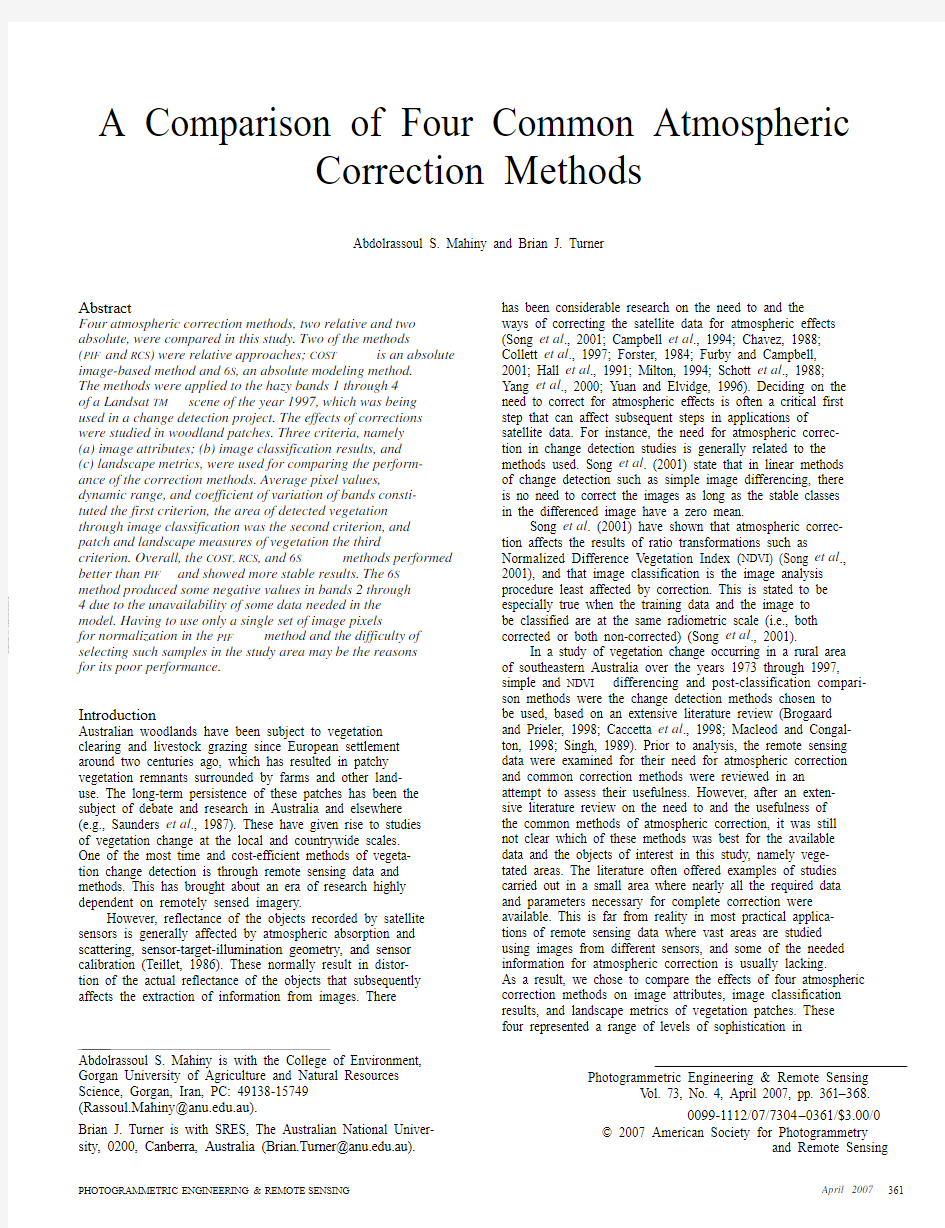
The study area was the catchment of the Boorowa River in southern New South Wales, Australia, approximately 110 km northwest of Canberra (Figure 1). The availability of field data, long history of settlement, and vegetation clearing and accessibility were among the reasons for this choice. The catchment covers an area of about 220 thousand hectares and is relatively flat with undulating hills to the east, north, and west. Pastures, farmlands, remnant woodlands, and small towns are the major land-cover/land-use covering the area. The average annual rainfall ranges from 570 mm to 770 mm (Hird, 1991). The area has a warm climate with long summers and cool to cold winters. Studies show that the pre-European native vegetation of the area was composed of three categories: dry schlerophyll forest, woodlands and grasslands (Hird, 1991).

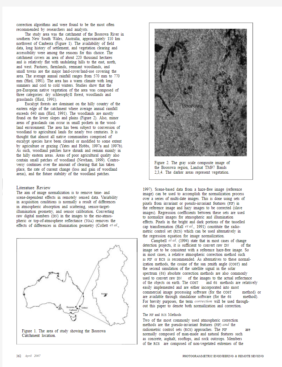
Eucalypt forests are dominant on the hilly country of the eastern edge of the catchment where average annual rainfall exceeds 640 mm (Hird, 1991). The woodlands are mostly found on the lower slopes and plains (Figure 2). Also, minor areas of grasslands can occur in small pockets in the wood- land environment. The area has been subject to conversion of woodland to agricultural lands for nearly two centuries. It is thought that almost all native communities comprised of eucalypt species have been cleared or modified to some extent by agriculture or grazing (Yates and Hobbs, 1997a and 1997b). As such, woodland patches have shrunk and remain mainly in the hilly eastern areas. Areas of poor agricultural quality also contain small patches of woodland (Newham, 1999). Contro- versy continues over the amount of clearing that has taken place, the rate of current change (loss and gain of woodland areas), and the future stability of the woodland patches.

Literature Review

The aim of image normalization is to remove time- and scene-dependent effects in remotely sensed data. Variability in acquisition conditions is normally a result of differences in atmospheric absorption and scattering, sensor-target- illumination geometry, and sensor calibration. Converting raw digital numbers (DN ) in the images to the exo-atmos- pheric or top-of-atmosphere reflectance (TOA ) removes the effects of differences in illumination geometry (Collett et al .,

Figure 1. The area of study showing the Boorowa Catchment location.

Figure 2. The gray scale composite image of the Boorowa region, Landsat TM97 Bands 2,3,4. The darker areas represent vegetation.

1997). Scene-based data from a haze-free image (reference image) can be used to accomplish the normalization process over a series of multi-date images. This is done using sets of pixels from invariant or pseudo-invariant features (PIF ) in the reference image and hazy images to be corrected (slave images). Regression coefficients between these sets are used to normalize images for atmospheric and illumination

effects. Pixels in the bright and dark portions of the tasselled cap transformation (Hall et al ., 1991) constitute the radio- metric control set (RCS ) which can be used alternatively in the regression equation for image normalization.

Campbell et al . (1994) state that in most cases of change detection projects, it is sufficient to convert raw DN of the image set to be consistent with a reference haze-free image. So in most cases, a relative atmospheric correction method such as PIF or RCS is recommended. As alternatives to these normal- ization methods, the cosine of the sun zenith angle (COST ) and the second simulation of the satellite signal in the solar

spectrum (6S ) absolute correction methods are also commonly used to convert raw DN of the images to the actual reflectance of the objects on earth. The COST and 6S methods are relatively easily implemented and are either incorporated into most commercial image processing software (for the COST method) or are available through standalone software (for the 6S method). For brevity purposes, the term correction will be used through- out this paper to denote both normalization and correction.

The PIF and RCS Methods

Two of the most commonly used atmospheric correction

methods are the pseudo-invariant features (PIF ) and the radiometric control sets (RCS ) approaches. The PIF are normally composed of man-made and natural features such as concrete, asphalt, rooftops, and rock outcrops. Members of the RCS are composed of non-vegetated extremes of the

362

April 2007

PHOTOGRAMMETRIC E NGINEERING & REMOTE S ENSING

tasselled cap transformation (Hall et al ., 1991) representing bright and dark objects in the imagery. For RCS , the green- ness and brightness components produced through the tasselled cap process are used to single out the extreme elements of the landscape such as deep water-bodies and

Based on the fact that normally, dark objects comprise

nearly 1 percent of the whole image reflectance (Chavez, 1988), the radiance of an absolutely dark object when it is haze-free will be:

sands for dark and bright sets, respectively.

L 1% ? (0.01E 0 cos TZ ) / (pd 2) (5)

The PIF and RCS are selected through the following criteria (Schott et al ., 1988; Hall et al ., 1991):

where d 2 is the squared sun-earth distance in astronomical

units. Hence, when the dark objects are hazy, the path PIF: {(Band4/Band3) ? t 1

AND (1)

radiance due to haze (L haze ) can be calculated by subtracting L 1% from the at-satellite radiance of hazy objects.

RCS: Dark sets ? {(greenness ? t 1)

AND

(brightness ? t 2)} L haze is then substituted in Equation 4, and the images are corrected band by band for atmospheric and radiometric noise. AND AND Bright sets ? {(greenness ? t 1) (brightness ? t 2)}

(2)

As is evident, the COST method uses no additional parameters other than those of the image and is able to approximate the effects of atmospheric gas absorption and where t 1 and t 2 are threshold values and the bands refer to Landsat TM data.

Geographically identical pixels are selected from the reference and slave images. Then, a simple linear regression is fitted between the raw DN in the slave and reference images for each band and used to normalise the slave image(s) to the reference one. The COST Method

Rayleigh scattering based on sun zenith angle.

The 6S Method

This model predicts the reflectance (?) of objects at the top of atmosphere (TOA ) using information about the surface reflectance and atmospheric conditions (Vermote et al ., 1997b). This information is provided through a minimum of input data to the model and incorporated features. The TOA reflectance can be estimated using the following formula:

COST is an image-based absolute correction method. It uses only the cosine of sun zenith angle (cos (TZ )) as an accept- able parameter for approximating the effects of absorption by atmospheric gases and Rayleigh scattering, hence the name COST . In using the model, DN of the images are first converted to radiance through the following formula (Chavez, 1988):

L sat ? (Lmin ? (Lmax ? Lmin )/DN max ) DN

(3)

r ? (p L sat d 2) / (E 0 cos TZ )

The surface reflectance (Ref) free from atmospheric effects is estimated as:

Ref ? [(Ar ? B ] / [1 ? (g (Ar ? B ))]

where A ? 1/??, B ? ??/?, ? is the global gas transmit- tance, ? is the total scattering transmittance, and ? is the (6)

(7)

where L sat is the spectral radiance at the sensor, Lmin is the minimum spectral radiance for a given band, Lmax is the maximum spectral radiance for a given band, and DN max is

the maximum digital number of the image range.

The values of Lmin and Lmax for each Landsat band are given by Markham and Barker (1986).

Then, the radiance is converted to reflectance of the objects at the Earth‘s surface using the following formula:

spherical albedo (UNESCO, 1999). Alpha, beta, and gamma are constants generated from running the model. The minimum data set needed to run the 6S model is the meteorological visibility, type of sensor, sun zenith and azimuth, date and time of image acquisition, and latitude and longitude of scene center. Using the input data and the embedded features, the model produces variables to assess the surface reflectance.

Ref ? p (L sat ? L haze ) / (E 0cos TZ )

(4)

Data and Methods where Ref is the reflectance at the Earth surface, L sat is the spectral radiance at the sensor, L haze is the path radiance, E 0 is the mean solar exo-atmospheric irradiance, and TZ is the mean solar angle. E 0 is obtained from Table 4 of the Markham and Barker (1986) publication.

The first step in calculating the path radiance (L haze ) is selection of the DN haze through one of the following ways:

· By looking at the image histogram and finding the minimum · By looking at areas of known zero reflectance like large deep

water-bodies and assuming that any value in the raw image

in these areas other than zero represents haze effects (although sediments and microscopic plants may obscure · By using software which automatically finds the DN for haze

· By defining other dark objects such as shadows and looking

for non-zero values in these areas. Principal components analysis or the tasselled cap transformation can be used for segmenting the shadows.

Then, the haze DN value is converted to at-satellite radiance for each band using Equation 4.

Overview

For the change detection study, a Landsat MSS scene for 1973

and a TM scene for 1997 were obtained (Table 1). This was done to provide the most extensive time frame for the change detection. From examination of the band histograms and actual DN values of dark water bodies, the MSS 1973 bands were found haze-free, so no correction was needed for them. On the other hand, examination of histograms of the TM 1997 bands revealed that the first three bands were contaminated with a moderate amount of haze that required atmospheric correction (Table 2). For the PIF and RCS relative atmospheric correction methods, a haze-free reference image was required. A TM scene from 1991 was the only haze-free image set available. It was recognized that using data so far apart in time might introduce difficulties due to sensor degradation or changes in the landscape. However, due to a lack of other suitable image data, the TM 1991 was chosen for the normalisation task. Field data recently collected were available to test the accuracy of image classification. Additionally, a 2002 SPOT XS image was acquired and used to assess the accuracy of classifi- cation. Because of the high spatial resolution of the SPOT XS image (10-meters) and high accuracy of its classification (99

PHOTOGRAMMETRIC ENGINEERING & REMOTE SENSING

April 2007

363

(Band7 ? t 2)

DN representative of haze values (Chavez, 1988); this);

value and applies a dark-object subtraction correction; or

T ABLE1.I MAGE D ATA S ETS U SED IN THE S TUDY AND THE S PECIFIC

I NFORMATION N EEDED FOR C ORRECTION

Sun

Imagery Date Zenith Azimuth D2COS TZ Landsat MSS18 Jan. 197322.910301.900 1.020.92 Landsat TM8 Feb. 199144.74076.1500.970.71 Landsat TM22 Oct. 199738.91061.800 1.010.77 SPOT 5 XS18 Nov. 200240.79052.300—

T ABLE2.I MPROVING THE S ELECTION OF DN haze V ALUES FOR B ANDS U SING THE M ILTON S PREADSHEET AND THE M ETHOD D EVELOPED BY C HAVEZ Fragstats ver. 2 (McGarigal and Marks, 1995) software was

used for landscape analysis.

Correction Methods Applied

PIF Normalization

For the PIF normalization, the relatively haze-free TM1991 was used as a reference. Then, pseudo-invariant features, consisting mainly of rock outcrops, bare soils, and built-up

areas were segmented using bands 3, 4, and 7 of the TM

1991 and TM1997 scenes, respectively.

For TM1991, a total of 3,155 pixels were singled out as

the PIF set. This was done in two stages. First, the TM1991 band 4 was divided by band 3. Then, by trial and error

Initial Refined

Imagery Band DN haze L haze (using known urban areas, water-bodies, and rock outcrops

on the division band), a DN value of 1.0 was chosen as the threshold value (t1) that separated the image into urban

TM22 Oct. 9715050.0 2.48

21315.2 1.15

3911.80.53

40 5.70.11

50 5.30.00

70 3.80.00

to 100 percent on classifying woody vegetation) tested by

visual evaluation and field data, this image was used as ground

truth for accuracy assessment.

The four methods of atmospheric correction were

applied to the TM1997 image and image attributes, image classification results, and landscape metrics were investi-

gated to compare the methods.

Average reflectance of woodlands, and the entire bands

of the image together with the dynamic range and coefficient

of variation were the image attributes evaluated. The dynamic

range of the bands is an important feature because it shows

the amount of fine detail and extractable information (Yang

and Lo, 2000). Hence, in a relative sense, any atmospheric correction method that produces wider dynamic ranges will

be of greater value for image classification. The frequency distribution of image values is another important measure

reflecting separability of clusters in an image (Yang and Lo, 2000). As a variable representing the frequency distribution,

the coefficient of variation (CV) was selected for comparing

the methods.

Landscape attributes are generally studied at three

scales: patch, class, and landscape (McGarigal and Marks,

1995). In this research, patch refers to the isolated remnant vegetation areas. The patches of vegetation can be grouped

into size classes or other categories. The whole landscape

mosaic containing patches, corridors of vegetation connect-

ing them, and the background matrix is studied through

the landscape metrics. It is assumed that any major change

in the bands‘ attributes will be reflected in the landscape

metrics. In order to assess the effects of the correction

methods on landscape metrics, the detected woodlands in

the classified TM1997 image were subjected to an adaptive

3 ? 3 box filter for removing single pixels. Woodland

patches less than 0.5 hectare were also removed, and the

remaining patches were classified into the following size

classes (in hectares): 0.5 to 1, 1 to 5, 5 to 10, 10 to 20, 20 to

50, 50 to 100, and more than 100.

Then, the number of patches and percent of landscape occupied by different patch-size classes were compared for

the correction methods. Total area of patches, patch-density,

mean patch-size, and landscape shape index together with

nearest neighbor and proximity indices were the landscape

metrics studied. IDRISI ver. 3.2 and ENVI ver. 3.4 software

were used for remote sensing analyses. The raster version of areas, water-bodies, and rock outcrops as one class and

other land-cover as the second class. Second, the DN values between 11 and 173 (t2) were used for segmenting man-

made features and vegetation on TM1991 band 7. Intersect-

ing the two resultant images with a logical AND gave the

final PIF set including only urban areas, rock outcrops, and

bare soils (Equation 1).

For TM1997,a total of3,577pixels were collected as the PIF set using t1and t2thresholds of0.9and9to238, respectively.The relatively low number of dark and bright pixels is due to most of the area being agricultural land and remnant woodlands.The coefficients of regres-sion between the bands were then used to normalise bands1through5,and7of TM1997relative to that of TM1991.

RCS Normalization

For the RCS method, a tasselled cap transformation was

applied to TM1991 and TM1997 bands 1 through 5 and 7. Then, the greenness and brightness components were

examined interactively for bright and dark objects. This

resulted in the selection of 973 bright and 33,672 dark

pixels for TM1991 and 1,416 bright and 30,469 dark pixels

for TM1997. Regression coefficients of the sets were calcu-

lated for the TOA reflectance of each band and then applied

to the bands to normalise TM1997 to TM1991.

COST Method

For the COST method,initial DN haze values were selected through histogram evaluation and then refined using gain and offset values(Table2).The refined DN haze values were calculated employing an Excel?spreadsheet,devel-oped by Milton(1994).The spreadsheet has been con-structed using the ideas of Chavez(1988)on improving atmospheric correction procedures.The horizontal visibil-ity was50km for the image date(Commonwealth Bureau of Meteorology,personal communication,2003)and

the haze DN value for the first band was50.Hence,the atmosphere was relatively clear at the time of satellite overpass,and a relative scattering model representing a clear atmosphere was chosen for the calculations in the Milton spreadsheet(see Chavez,1988).The results of the spreadsheet application and COST correction method are shown in Table 2.

The calculated L haze for each band was substituted in Equation 4 for the COST method. Automatic selection of

DN haze values by commercial software can be misleading,

because it normally results in the selection of the lowest

non-zero number with a very low frequency in the his-

togram for the haze value. However, in most cases, the

histogram minimum just represents noise in the imagery and

values slightly larger than that with a higher frequency of

pixels should be selected (Figure 3; Table 3).

364April2007PHOTOGRAMMETRIC E NGINEERING&REMOTE S ENSING

T ABLE 4. P ARAMETERS D ERIVED FROM THE 6S M ODEL

AND S UBSEQUENT C ALCULATIONS

Parameter

TM1

TM2

TM3

TM4

Global gas 0.98 0.91 0.93 transmittance Total scattering 0.76 0.84 0.88 0.92 transmittance Reflectance 0.07 0.04 0.02 0.01 Spherical albedo 0.15 0.10 0.07 0.04 A 1.32 1.29 1.20 1.17 B

?0.09

?0.04

?0.02

?0.01

Figure 3. Hypothetical figure showing the difference between automatic and manual selection of DN haze value.

T ABLE 3. C OMPARISON OF DN haze S ELECTION T HROUGH M ANUAL H ISTOGRAM A NALYSIS AND A UTOMATIC M ETHOD. ―A‖ S TANDS FOR A UTOMATIC AND ―M‖ FOR

H ISTOGRAM M ETHOD

Band 2

Band 3

Band 4

Image Attributes

The expected reflectance pattern for eucalypt woodlands is a relatively low reflectance in the blue band (band 1), a rise in the green band (band 2), a fall in the red band (band 3), followed by a sharp rise in the near infrared band (band 4) (e.g., Huang et al ., 2004). The RCS and PIF corrected data showed this pattern (Figure 4). However, the 6S method gave lower than expected reflectance values for bands 1 and 2, and the COST correction resulted in relatively lower reflectance in the green band. The TOA reflectances (uncorrected for atmospheric effects) were high in the blue band, a not unexpected result.

The COST method generated the widest dynamic range in most bands followed by the 6S method (Table 5). The PIF A 42 1 12 A 6 1 method generated the lowest dynamic range except in band 48 1 M

14 3 50 3 15 43 M

9

10 M

51 16 1054 32 52 21 17 5550 60 53 127 18 5426 534 54 489 19 5353 13 2219 55 1167 20 9986 14 4449 56 2059 21 36434 15 9613 57

3604 22

54221 16

21612

DN

four in which it was greater than RCS .

In order to test the differences statistically, a hundred points were randomly selected across the image and areas of 62 hectares in size were digitised around them. Then, the dynamic range of the random areas across the bands were measured and subjected to analysis of variance (ANOVA ) using Statistica ver. 5.2 (Statsoft, Inc., 1999). The analysis showed significant differences between the mean dynamic ranges for the COST , 6S, RCS , and TOA methods over all four bands. Tukey‘s honestly significant difference (HSD ) test was carried out on all pairs of means to reveal the significant differences between pairs. As can be seen from Table 5, the 100 799 0 2190 PIF range was significantly less than that of the other

1

97 716 7991 methods in bands 1 through 3. The COST and 6S produced a 248 No Haze

3 336

4 55

5 5 892

2208 14314 6289 3 16595 13618 4 16191 16052 11612

similar dynamic range in most cases.

Analysis of the different bands in relation to the coefficient of variation (CV ) showed that the 6S method

6456 10377 6 7396 17239 5959 7

4756 8 21761 4148 4103 9

13718

3509

4211

6S Modeling

For the 6S atmospheric correction, a minimum data set

composed of date, sun zenith, azimuth angles, and horizontal visibility was used. The horizontal visibility was available from weather stations located in the region (Commonwealth Bureau of Meteorology, personal communication). The Msixs software ver. 6.2 (Vermote et al ., 1997a) was used for the calculations. The result of running the 6S model for the first four bands of the TM 1997 dataset is given in Table 4. The TOA reflectance for each band was converted to ground reflectance using Equation 7.

Results and Discussion

The effects of the correction methods at three levels of (a) image attributes, (b) image classification results, and (c) landscape metrics are explained as follows.

Figure 4. Average reflectance of woodlands for the correction methods.

PHOTOGRAMMETRIC ENGINEERING & REMOTE SENSING

April 2007

365

generated the largest CV for bands 1 and 3, and the RCS method gave the highest CV for band 2 followed by the 6S method (Table 6). The PIF method produced the smallest average CV in most bands.

Statistical analysis of the random areas for the four

bands treated with the COST, 6S, RCS, PIF, and TOA methods showed significant differences in terms of coefficient of variation. Tukey‘s HSD test applied to the CV for the four bands revealed that in most cases, for bands 1 through 3 the methods of correction are significantly different from each other. There was little separability for band 4.

Image Classification

In the post-classification comparison method, images for

each date are classified individually, and the results of classification are compared through cross-tabulation. To

implement this method, all of the six bands of the corrected

and uncorrected (raw) TM1997 image were used in a maximum likelihood classification with a set of training

areas selected from the classified SPOT XS image. The images were initially classified into two categories of woody and

non-woody areas. The SPOT classification image was also

used to validate the TM1997 classification. Differences were detected between the results of the classification of the

corrected bands and that of the uncorrected bands. In this

regard, the proportion of woodlands to the whole image

was nearly equal for the COST, 6S, and RCS methods. The

PIF method indicated a smaller proportion of woodlands

compared to the other methods and the TOA image showed the highest proportion (Figure 5).

The additional area of detected woodlands resulting

from the correction methods was validated by the classified

and highly accurate SPOT image. Then, this additional area

for each correction method was compared to the uncorrected image. The TOA image detected the greatest additional area

of woodland followed by the RCS, 6S, and the COST. The PIF

method produced the smallest area of additional woodland.

SPOT image validation of the corrected classified images confirmed an average additional 1,195 hectares of wood-

T ABLE5.T UKEY‘S HSD T EST ON D YNAMIC R ANGE OF R EFLECTANCE OF

TM97(A LPHA? .05)

TM Bands Correction Methods and Means

16S COST RCS TOA PIF ?:.060.058.057.045.033 2COST6S RCS TOA PIF ?:.087.0863.081.067.048 3COST6S TOA RCS PIF

Figure 5.Difference in classification of woody and

non-woody areas as a result of correction methods

lands resulting from application of the correction methods. However, the methods failed to make an average area of

277 hectares of woodlands discernible to the classifier as compared to the non-corrected image. Table 7 shows the differential amount of woodland detected by the maximum likelihood classification of the non-corrected and corrected

TM1997 images.

The differential areas of woodland detected by the correction methods were overlaid to investigate their spatial overlap. Of the validated extra woodlands detected by different methods of correction, only 327 hectares (27.3 percent) were detected by all four methods. This shows that

the correction methods behave differently in making areas of woodlands discernible to the classifier. In other words, apart from the fact that the corrections have improved the classifi-cation results, each method has affected the process by identifying woodlands in different locations. Hence, it is expected that the distribution of patches across the land-

scape and the related landscape indices will also be differ-

ent for the correction methods used.

Landscape Metrics

Analysis of the patch metrics revealed that the number of patches over the landscape was greatest in the TM1997 image corrected by 6S and TOA followed closely by the RCS and COST methods. Again, the PIF method resulted in a smaller number of patches as compared to the other meth-

ods but the number was still greater than that determined

?:.125.116.097.063from the raw image (Table 8). This supports the argument

4COST6S TOA PIF RCS ?:.440.391.342.262.224

T ABLE6.T UKEY‘S HSD T EST ON C OEFFICIENT OF V ARIATION OF TM97

(A LPHA? .05)that a larger dynamic range and CV also give rise to detec-tion of finer detail in the images since the PIF method returned low values for these two measures.

TM Bands Correction Methods and Means

16S COST RCS PIF TOA ?:31.4416.0913.659.70 6.84 2RCS6S COST TOA PIF

?:28.1623.3818.0312.028.88 36S COST TOA RCS PIF

?:31.3125.7620.3919.8416.47 4COST TOA RCS PIF6S

?:21.0220.6818.9218.8717.73

T ABLE7.A REA OF W OODLANDS D ETECTED IN THE C ORRECTED I MAGES AND N OT-DETECTED IN THE R AW I MAGES(A) AND THE R EVERSE(B)

Amount of Woodland (ha) Subtraction Operation A B Raw - 6S1,213252 Raw - COST

1,168278 Raw - PIF956244 Raw - RCS1,226328 Raw - TOA1,412283

366April2007PHOTOGRAMMETRIC E NGINEERING&REMOTE S ENSING

T ABLE 8. C OMPARISON OF THE P ATCH M ETRICS FOR THE

C ORRECTION M ETHODS

No. of Patches

Class (ha) PIF

RCS

COST

6S

TOA

(uncorrected)

.5–1 884 913 909 875 912 801 1–5 784 820 778 838 811 735 5–10 135 127 138 141 149 118 10–20 70 67 78 80 72 47 20–50 48 46 60 56 43 50–100 19 20 21

18 100? 24 22 25 23 26 TOTAL

1,964 2,015

2,007

2,032

1,791

T ABLE 9. C OMPARING

THE E FFECT OF C ORRECTION ON THE D ISTRIBUTION OF

P ATCHES A CROSS L ANDSCAPE

Correction Method

Indices 6S

COST

PIF RCS TOA

Raw Mean Nearest 605

629 665

640

635

658 Neighbor (m) Mean Proximity 4.7 5.2

4.9 4.2 7.5

10

Index

T ABLE 10. C OMPARISON OF S ELECTED L ANDSCAPE I NDICES FOR THE

C ORRECTION M ETHODS

Method

Area (ha) Patches (#100 ha) Size (ha) Shape Index PIF

15,763 1,964 12.45 8.02 65.54 RCS

16,019 2,015 12.57 7.95 66.38 COST

16,091 2,007 12.47 8.01 66.26 6S

16,190 2,032 12.55 7.96 66.74 TOA

16,467 2,032 12.34 8.10 66.45 Raw 14,546

1,791

12.31

8.12

63.63

The correction methods were also found more efficient in detecting the smallest areas of vegetation. In this regard, the RCS, TOA , and the COST methods produced the best results (Table 8).

As is clear from Table 9, the distribution of patches for the different methods of correction varies greatly. The smallest nearest neighbour was found with the 6S method, followed by COST, TOA , and RCS . With the PIF method, this index was even greater than the raw image suggesting that the method has been able to distinguish the larger patches at the expense of the smaller ones. Also, the smallest proximity index was detected using the RCS method followed by the 6S and PIF . The COST method was better than the TOA , and the raw image performed very poorly in this connection.

The results shown in Table 10 also affirm these conclu- sions. As is clear from this table, the correction methods have produced images with more patches than detected in the raw image.

Conclusion

Atmospheric correction methods used in this study showed an effect on image attributes, vegetation change detection, and the landscape metrics. Based solely on this fact, atmos-

pheric correction is judged a necessary step with regard to

the aims and specifications of the broader research study. However, it was shown that each method behaved somewhat differently. When it comes to choosing one of the methods for atmospheric correction, the user should be aware that the methods have their own advantages and disadvantages. Each of the COST, RCS , or 6S methods can be equally used where slight differences in the detected woodlands in the form of small and scattered remnants are deemed unimportant. When studying woodlands for the purpose of biodiversity or wildlife habitats, even a few extra hectares and their spatial arrangement can cause profound effects on the final results. In these instances, choosing the right correction method becomes crucial. Around 1,195 extra hectares of woodland have been detected in this study as a result of corrections applied to the TM 1997 compared to the raw TM 1997 image and confirmed by the reference classified SPOT image. The extra woodland has been found dispersed across the landscape. This is about 8.9 percent of the total woodland coverage in the area of study. The difference between the corrected images and the raw image and the discrepancy between the results of the correction methods may be ecologically important. For example, the extra woodlands act as connectors of the patches, increasing the size, changing the shape and other attributes of the patches that affect the decisions on the faunal habitat quality, biodiversity, and the persistence of the patches. The correction methods each tended to increase the accuracy of the classification through distinguishing the vegetation patches in different parts of the landscape. In other words, what was classified as a patch of woodland in a given correction method, might not be so detected by another method. The 6S, RCS, COST , and PIF along with the TOA tended to detect more small patches compared with the raw image. Thus, the proximity index and mean nearest neighbour decreased with the above corrections. This is because of the higher dynamic range in the data as a result of the corrections.

With any of the correction methods, the time needed to carry out the procedure and the feasibility of application can become very important. The time required for each method can be a crucial factor when many sets of imagery are used. The RCS method required more analyst time than the PIF . The absolute and modeling methods of COST and 6S were applied to the imagery in considerably less time than the PIF and RCS methods. It is suggested that selection of a small sample and relying on just one sample may have caused the PIF method to perform poorly. The only critical factor with the COST method is selection of the correct DN haze values. In this study, the automatic selection of DN haze did not produce the same results as the manual method. Usually, a combina- tion of automatic selection of DN haze and visual inspection of the histogram is required for this purpose. For the 6S model to produce accurate results, detailed data on the atmospheric condition is required. Often this information is not available. Using only the available information on parameters and default values for the rest may cause the model to produce anomalous results such as negative values. However, the number of these pixels is likely to be minimal compared to the whole scene (as in this study), and hence it may not affect the final results greatly.

The COST, RCS , and 6S methods produced relatively consistent results across the bands when the dynamic range and coefficient of variation were considered. Also, with image classification and landscape indices, the COST , 6S , and RCS performed better than the PIF and raw image and distinguished more patches. It was shown that merely converting raw image data to exo-atmospheric reflectance could enhance the final results. In most cases where a

PHOTOGRAMMETRIC ENGINEERING & REMOTE SENSING

April 2007

367

relatively accurate correction fulfils the needs of study, the image-based correction method of the COST is an efficient way of removing atmospheric effects while saving time. Where possible, the RCS method offers a good way of correcting images. In case of a need for a speedy correction with relatively correct results, the 6S modelling procedure with minimum input can be employed. It is suggested that

for the PIF method to produce acceptable results, a large sample of pixels be selected from across the image. If this cannot be achieved, applying the method is better than

using the non-corrected image at the very least. To borrow a sentences from Keith et al. (2002), although using in a different context, this study has shown that making correc-

tion through one of the COST, RCS, or 6S methods is more important than quibbling about which of these correction methods to use.

Acknowledgments

The authors wish to thank the authorities at the Gorgan University of Agricultural Sciences and Natural Resources

of Iran for financially supporting the Ph.D. research for

the principal author. Dr. Gary Richards of the Australian Greenhouse Office, Canberra, kindly provided some of the remote sensing data. Also, the Boorowa Shire made the required SPOT image available to this study. Dr. Lachlan Newham offered other needed remote sensing data, and Ms. Suzanne Furby of the Bureau of Rural Sciences provided technical advice. Several reviewers provided helpful com-ments. We thank them all greatly.

References

Brogaard,S.,and S.Prieler,https://www.360docs.net/doc/d89117856.html,nd cover in the Horqin Grasslands,North China.Detecting Changes Between1975and

1990by Means of Remote Sensing, International Institute for

Applied System Analysis, Austria, URL: http://www.iiasa.ac.at/

Publications/Documents/IR-98-044.pdf (last date accessed:

23 December 2006).

Caccetta, P.A., N.A. Campbell, F. Evans, S.L. Furby, H.T. Kiiveri, and J.F. Wallace, 1998. Mapping and Monitoring Land Use and

Condition Change in the South-West of Western Australia Using

Remote Sensing and Other Data, CSIRO Mathematical and

Information Sciences, URL: http://www.cmis.csiro.au/RSM

/research/pdf/CaccettaP_europa2000.pdf (last date accessed:

23 December 2006).

Campbell, N., S. Furby, and B. Fergusson, 1994. Calibrating Images from Different Dates, CSIRO Mathematical and Information

Sciences, URL: http://www.cmis.csiro.au/rsm/research/index.htm (last date accessed: 23 December 2006).

Chavez, P.S., 1988. An improved dark-object subtraction technique for atmospheric scattering correction of multispectral data,

Remote Sensing of Environment, 24:459–479.

Collett, L.J., B.M. Goulevitch, and T.J. Danaher, 1997. SLATS Radiometric Correction:A Semi-automated,Multi-stage Process

for the Standardisation of Temporal and Spatial Radiometric

Differences, Queensland Department of Natural Resources, URL:

https://www.360docs.net/doc/d89117856.html,.au/slats/pdf/arspc9_rad_corrections1.pdf (last date accessed: 23 December 2006).

Forster, B.C., 1984. Derivation of atmospheric correction procedures for Landsat MSS with particular reference to urban data,

International Journal of Remote Sensing, 5:799–817.

Furby, S.L., and N.A. Campbell, 2001. Calibrating images from different dates to ?like-value‘ digital counts, Remote Sensing of

Environment, 77:186–196.

Hall, F.G., D.E. Strebel, J.E. Nickeson, and S.J. Goetz, 1991. Radio-metric rectification – Toward a common radiometric response

among multidate, multisensor images, Remote Sensing of

Environment, 35:11–27.Hird, C., 1991. Soil Landscapes of the Goulburn1:250,000, Soil Conservation Service of NSW, Sydney, Australia.

Huang, Z., B.J. Turner, S.J. Dury, I.R. Wallis, and W.J. Foley, 2004.

Estimating foliage nitrogen concentration from HYMAP data

using continuum removal analysis, Remote Sensing of Environ-

ment, 93:18–29.

Macleod, R.D., and R.G. Congalton, 1998. Quantitative comparison of change-detection algorithms for monitoring eelgrass from

remotely sensed data, Photogrammetric Engineering&Remote

Sensing, 64(2):207–216.

Markham, B.L., and J.L. Barker, 1986. Landsat MSS and TM post-calibration dynamic ranges, exoatmospheric reflectances and

at-satellite tmperatures, EOSAT Landsat Technical Notes,

1:3–8.

McGarigal, K., and B.J. Marks, 1995. FRAGSTATS:Spatial Pattern Analysis Program for Quantifying Landscape Structure, USDA

Forest Service, URL: https://www.360docs.net/doc/d89117856.html,/pubs/viewpub.

jsp?index?3064, (last date accessed: 23 December 2006). Milton, E.J., 1994. Teaching atmospheric correction using a spread-sheet, Photogrammetric Engineering&Remote Sensing, 60(6):

751–754.

Newham, L.T.H., 1999. The Use of Remote Sensing and Geographic Information Systems in Landcare Resource Assessment and

Planning, M.Sc. thesis, Department of Forestry, The Australian

National University, Canberra.

Saunders, D.A., G.W. Arnold, A.A. Burbidge, and A.J.M. Hopkins, 1987. Nature Conservation:The Role of Remnants of Native

Vegetation, Surrey Beaty & Sons, NSW, Australia.

Schott, J.R., C. Salvaggio, and W.J. Volchok, 1988. Radiometric scene normalization using pseudoinvariant features, Remote

Sensing of Environment, 26:1–16.

Singh, A., 1989. Digital change detection techniques using remotely-sensed data, International Journal of Remote Sensing, 10:

989–1003.

Song, C.,C.E.Woodcock,K.C.Seto,M.P.Lenney,and S.A.

Macomber, 2001. Classification and change detection using

Landsat TM data: When and how to correct atmospheric

effects?, Remote Sensing of Environment, 75:230–244.

Teillet, P.M., 1986. Image correction for radiometric effects in remote sensing, International Journal of Remote Sensing,

7:1637–1651.

UNESCO, 1999. Applications of satellite and airborne image data to coastal management, Coastal Region and Small Island Papers4, UNESCO, Paris, URL: https://www.360docs.net/doc/d89117856.html,/tcmweb/bilko/ (last

date accessed: 23 December 2006).

Vermote, E.F., D. Tanre, J.L. Beuze, M. Herman, and J.J. Morcrette, 1997a. Msixs,Release6.4, Université des Sciences et Technolo-

gies de Lille, Lille, France, URL: http://www-loa.univ-lille1.fr

/Msixs/msixs_gb.html (last date accessed: 23 December 2006). Vermote, E.F., D. Tanre, J.L. Deuze, M. Herman, and J.J. Morcrette, 1997b. Second simulation of the satellite signal in the solar

spectrum, 6S: An overview, IEEE Transactions on Geoscience

and Remote Sensing, 35:675–686.

Yang, X.J., and C.P. Lo, 2000. Relative radiometric normalization performance for change detection from multi-date satellite

images, Photogrammetric Engineering&Remote Sensing, 66(8): 967–980.

Yates, C.J., and R.J. Hobbs, 1997a. Woodland restoration in the western Australian wheatbelt: A conceptual framework using a

state and transition model, Restoration Ecology, 5:28–35. Yates, C.J., and R.J. Hobbs, 1997b. Temperate Eucalypt woodlands:

A review of their status, processes threatening their persistence

and techniques for restoration, Australian Journal of Botany,

45:949–973.

Yuan, D., and C.D. Elvidge, 1996. Comparison of relative radiomet-ric normalization techniques, ISPRS Journal of Photogrammetry

and Remote Sensing, 51:117–126.

(Received 26 April 2005; accepted 07 September 2005; revised

01 November 2005)

368April2007PHOTOGRAMMETRIC E NGINEERING&REMOTE S ENSING