B-spline Curves(B样条曲线)

Motivation

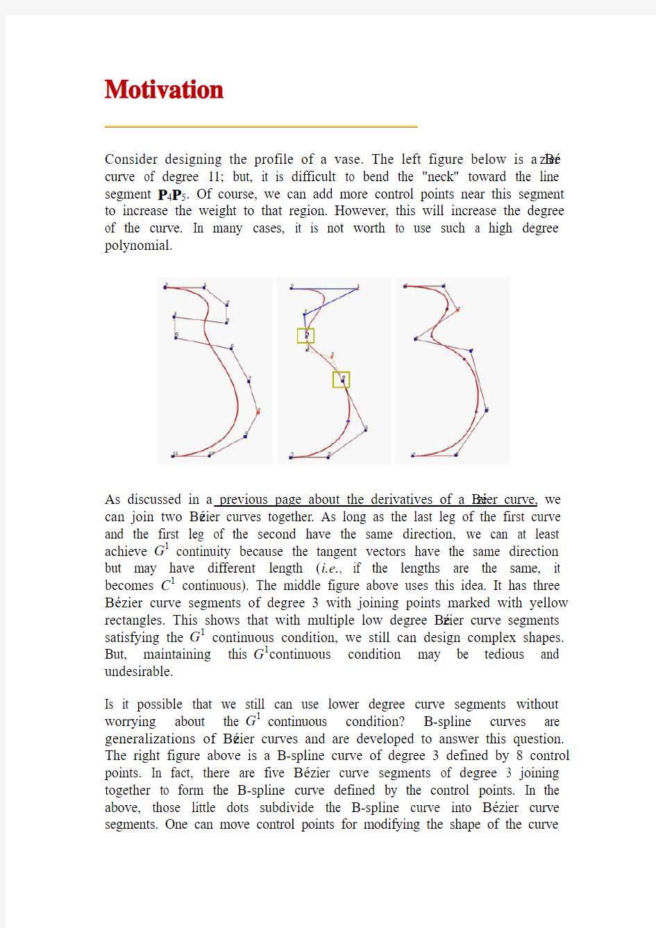
Consider designing the profile of a vase. The left figure below is a Bézier curve of degree 11; but, it is difficult to bend the "neck" toward the line segment P4P5. Of course, we can add more control points near this segment to increase the weight to that region. However, this will increase the degree of the curve. In many cases, it is not worth to use such a high degree polynomial.

As discussed in a previous page about the derivatives of a Bézier curve, we can join two Bézier curves together. As long as the last leg of the first curve and the first leg of the second have the same direction, we can at least achieve G1 continuity because the tangent vectors have the same direction but may have different length (i.e., if the lengths are the same, it becomes C1 continuous). The middle figure above uses this idea. It has three Bézier curve segments of degree 3 with joining points marked with yellow rectangles. This shows that with multiple low degree Bézier curve segments satisfying the G1 continuous condition, we still can design complex shapes. But, maintaining this G1continuous condition may be tedious and undesirable.

Is it possible that we still can use lower degree curve segments without worrying about the G1 continuous condition? B-spline curves are generalizations of Bézier curves and are developed to answer this question. The right figure above is a B-spline curve of degree 3 defined by 8 control points. In fact, there are five Bézier curve segments of degree 3 joining together to form the B-spline curve defined by the control points. In the above, those little dots subdivide the B-spline curve into Bézier curve segments. One can move control points for modifying the shape of the curve

just like what we do to Bézier curves. We can also modify the subdivision of the curve. Therefore, B-spline curves have higher degree of freedom for curve design.

Subdividing the curve directly is difficult to do. Instead, we subdivide the domain of the curve. Thus, if the domain of a curve is [0,1], this closed interval is subdivided by points called knots. Let these knots be 0 <= u0 <= u1 <= ... <= u m <= 1. Then, points C(u i)'s subdivide the curve as shown in the figure below and, consequently, modifying the subdivision of [0,1] changes the shape of the curve.

In summary, to design a B-spline curve, we need a set of control points, a set of knots and a set of coefficients, one for each control point, so that all curve segments are joined together satisfying certain continuity condition. The computation of the coefficients is perhaps the most complex step because they must ensure certain continuity conditions. Fortunately, this computation is usually not needed in this course. We only need to know their characteristics for reasoning about B-spline curves.

B-spline Basis Functions:

Definition

Bézier basis functions are used as weights. B-spline basis functions will be used the same way; however, they are much more complex. There are two interesting properties that are not part of the Bézier basis functions, namely: (1) the domain is subdivided by knots, and (2) basis functions are not non-zero on the entire interval. In fact, each B-spline basis function is non-zero on a few adjacent subintervals and, as a result, B-spline basis functions are quite "local".

Let U be a set of m + 1 non-decreasing numbers, u0 <= u2 <= u3 <= ... <= u m. The u i's are called knots, the set U the knot vector, and the half-open interval [u i, u i+1) the i-th knot span. Note that since some u i's may be equal, some knot spans may not exist.If a knot u i appears k times (i.e., u i = u i+1 = ... = u i+k-1), where k > 1, u i is a multiple knot of multiplicity k, written as u i(k). Otherwise, if u i appears only once, it is a simple knot. If the knots are equally spaced (i.e., u i+1 - u i is a constant for 0 <= i <= m - 1), the knot vector or the knot sequence is said uniform; otherwise, it is non-uniform. The knots can be considered as division points that subdivide the interval [u0, u m] into knot spans. All B-spline basis functions are supposed to have their domain on [u0, u m]. In this note, we use u0 = 0 and u m = 1 frequently so that the domain is the closed interval [0,1].

To define B-spline basis functions, we need one more parameter, the degree of these basis functions, p. The i-th B-spline basis function of degree p, written as N i,p(u), is defined recursively as follows:

The above is usually referred to as the Cox-de Boor recursion formula. This definition looks complicated; but, it is not difficult to understand. If the degree is zero (i.e., p = 0), these basis functions are all step functions and this is what the first expression says. That is, basis function N i,0(u) is 1 if u is

in the i-th knot span [u i, u i+1). For example, if we have four knots u0 = 0, u1 = 1, u2 = 2 and u3 = 3, knot spans 0, 1 and 2 are [0,1), [1,2), [2,3) and the basis functions of degree 0 are N0,0(u) = 1 on [0,1) and 0 elsewhere, N1,0(u) = 1 on [1,2) and 0 elsewhere, and N2,0(u) = 1 on [2,3) and 0 elsewhere. This is shown below:

To understand the way of computing N i,p(u) for p greater than 0, we use the triangular computation scheme. All knot spans are listed on the left (first) column and all degree zero basis functions on the second. This is shown in the following diagram.

To compute N i,1(u), N i,0(u) and N i+1,0(u) are required. Therefore, we can compute N0,1(u), N1,1(u), N2,1(u), N3,1(u) and so on. All of these N i,1(u)'s are written on the third column. Once all N i,1(u)'s have been computed, we can compute N i,2(u)'s and put them on the fourth column. This process continues until all required N i,p(u)'s are computed.

In the above, we have obtained N0,0(u), N1,0(u) and N2,0(u) for the knot vector U = { 0, 1, 2, 3 }. Let us compute N0,1(u) and N1,1(u). To compute N0,1(u), since i = 0 and p = 1, from the definition we have

Since u0 = 0, u1 = 1 and u2 = 2, the above becomes

Since N0,0(u) is non-zero on [0,1) and N1,0(u) is non-zero on [1,2), if u is in [0,1) (resp., [1,2) ), only N0,0(u) (resp., N1,0(u) ) contributes to N0,1(u). Therefore, if u is in [0,1), N0,1(u) is uN0,0(u) = u, and if u is in [1,2),N0,1(u) is (2 - u)N1,0(u) = (2 - u). Similar computation gives N1,1(u) = u - 1 if u is in [1,2), and N1,1(u) = 3 - u if u is in [2,3). In the following figure, the black and red lines are N0,1(u) and N1,1(u), respectively. Note that N0,1(u) (resp., N1,1(u)) is non-zero on [0,1) and [1,2) (resp., [1,2) and [2,3)).

Once N0,1(u) and N1,1(u) are available, we can compute N0,2(u). The definition gives us the following:

Plugging in the values of the knots yields

Note that N0,1(u) is non-zero on [0,1) and [1,2) and N1,1(u) is non-zero on [1,2) and [2,3). Therefore, we have three cases to consider:

1.u is in [0,1):

In this case, only N0,1(u) contributes to the value of N0,2(u).

Since N0,1(u) is u, we have

2.u is in [1,2):

In this case, both N0,1(u) and N1,1(u) contribute to N0,2(u). Since N0,1(u) = 2 - u and N1,1(u) = u - 1 on [1,2), we have

3.u is in [2,3):

In this case, only N1,1(u) contributes to N0,2(u). Since N1,1(u) = 3 - u on [2,3), we have

If we draw the curve segment of each of the above three cases, we shall see that two adjacent curve segments are joined together to form a curve at the knots. More precisely, the curve segments of the first and second cases join together at u = 1, while the curve segments of the second and third cases join at u = 2. Note that the composite curve shown here is smooth. But in general it is not always the case if a knot vector contains multiple knots.

Two Important Observations

Since N i,1(u) is computed from N i,0(u) and N i+1,0(u) and since N i,0(u) and N i+1,0(u) are non-zero on span [u i, u i+1) and [u i+1, u i+2), respectively, N i,1(u) is non-zero on these two spans. In other words, N i,1(u) is non-zero on [u i, u i+2). Similarly, since N i,2(u) depends on N i,1(u) and N i+1,1(u) and since these two basis functions are non-zero on [u i, u i+2) and [u i+1, u i+3), respectively, N i,2(u) is non-zero on [u i, u i+3). In general, to determine the non-zero domain of a basis function N i,p(u), one can trace back using the triangular computation scheme until it reaches the first column. The covered spans are the non-zero domain of this basis function. For example, suppose we want to find out the non-zero domain of N1,3(u). Based on the above discussion, we can trace back in the north-west and south-west directions until the first column is reached as shown with the blue dotted line in the following diagram. Thus, N1,3(u) is non-zero on [u1, u2), [u2, u3), [u3, u4) and [u4, u5). Or, equivalently, it is non-zero on [u1, u5).

In summary, we have the following observation:

Basis function N i,p(u) is non-zero on [u i, u i+p+1). Or,

equivalently, N i,p(u) is non-zero on p+1 knot spans [u i, u i+1),

[u i+1, u i+2), ..., [u i+p, u i+p+1).

Next, we shall look at the opposite direction. Given a knot span [u i, u i+1), we want to know which basis functions will use this span in its computation. We can start with this knot span and draw a north-east bound arrow and a south-east bound arrow. All basis functions enclosed in this wedge shape use N i,0(u) (why?) and hence are non-zero on this span. Therefore, all degree p basis functions that are non-zero on [u i, u i+1) are the intersection of this wedge and the column that contains all N i,p(u)'s. In fact, this column and the two arrows form an equilateral triangle with this column being the vertical side. Counting from N i,0(u) to N i,p(u) there are p+1 columns. Therefore, the vertical side of the equilateral triangle must have at most p+1 entries, namely N i,p(u), N i-1,p(u), N i-2,p(u), ..., N i-p+2,p(u), N i-p+1,p(u) and N i-p,p(u).

Let us take a look at the above diagram. To find all degree 3 basis functions that are non-zero on [u4, u5), draw two arrows and all functions on the vertical edges are what we want. In this case, they are N1,3(u), N2,3(u), N3,3(u), and N4,3(u). This is shown with the orange triangle. The blue (resp., red) triangle shows the degree 3 basis functions that are non-zero on [u3, u4) (resp., [u2, u3) ). Note that there are only three degree three basis polynomials that are non-zero on [u2, u3).

In summary, we have observed the following property.

On any knot span [u i, u i+1), at most p+1 degree p basis

functions are non-zero,

namely: N i-p,p(u), N i-p+1,p(u), N i-p+2,p(u), ..., N i-1,p(u)

and N i,p(u),

What Is the Meaning of the Coefficients?

Finally, let us investigate the meaning of the coefficients in the definition of N i,p(u). As N i,p(u) is being computed, it uses N i,p-1(u) and N i+1,p-1(u). The former is non-zero on [u i, u i+p). If u is in this half-open interval, then u -u i is the distance between u and the left end of this interval, the interval length is u i+p - u i, and (u - u i) / (u i+p - u i) is the ratio of the above mentioned distances and is always in the range of 0 and 1. See the diagram below. The second term, N i,p-1(u), is non-zero on [u i+1, u i+p+1). If u is in this interval, then u i+p+1 - u is the distance from u to the right end of this interval, u i+p+1 - u i+1 is the length of the interval, and (u i+p+1 - u) / (u i+p+1 - u i+1) is the ratio of these two distances and its value is in the range of 0 and 1. Therefore, N i,p(u) is a linear combination of N i,p-1(u) and N i+1,p-1(u) with two coefficients, both linear in u, in the range of 0 and 1.

Important Properties

Let us recall the definition of the B-spline basis functions as follows:

This set of basis functions has the following properties, many of which resemble those of Bézier basis functions.

1.N i,p(u) is a degree p polynomial in u

2.Nonnegativity -- For all i, p and u, N i,p(u) is non-negative

3.Local Support -- N i,p(u) is a non-zero polynomial on [u i,u i+p+1)

This has been discussed on previous page.

4.On any span [u i, u i+1), at most p+1 degree p basis functions are

non-zero, namely: N i-p,p(u), N i-p+1,p(u), N i-p+2,p(u), ..., and N i,p(u)

5.Partition of Unity -- The sum of all non-zero degree p basis

functions on span [u i, u i+1) is 1:

The previous property shows that N i-p,p(u), N i-p+1,p(u), N i-p+2,p(u), ..., and N i,p(u) are non-zero on [u i, u i+1). This one states that the sum of these p+1 basis functions is 1.

6.If the number of knots is m+1, the degree of the basis functions

is p, and the number of degree p basis functions is n+1, then m = n + p + 1:

This is not difficult to see. Let N n,p(u) be the last degree p basis function. It is non-zero on [u n, u n+p+1). Since it is the last basis function, u n+p+1 must be the last knot u m. Therefore, we have u n+p+1 = u m and n+p+1= m. In summary, given m and p, let n = m-p -1 and the degree p basis functions are N0,p(u), N1,p(u), N2,p(u), ..., and N n,p(u).

7.Basis function N i,p(u) is a composite curve of degree p polynomials

with joining points at knots in [u i, u i+p+1 )

The example shown on the previous page illustrates this property well.

For example, N0,2(u), which is non-zero on [0,3), is constructed from three parabolas defined on [0,1), [1,2) and [2,3). They are connected together at the knots 2 and 3.

8.At a knot of multiplicity k, basis function N i,p(u)

is C p-k continuous.

Therefore, increasing multiplicity decreases the level of continuity, and increasing degree increases continuity. The above mentioned degree two basis function N0,2(u) is C1 continuous at knots 2 and 3, since they are simple knots (k = 1).

The Impact of Multiple Knots

Multiple knots do have significant impact on the computation of basis functions and some "counting" properties. We shall look at two of them and

a calculation example will be provided on the next page.

1.Each knot of multiplicity k reduces at most k-1 basis functions'

non-zero domain.

Consider N i,p(u) and N i+1,p(u). The former is non-zero on [u i, u i+p+1) while the latter is non-zero on [u i+1, u i+p+2). If we move u i+p+2 to u i+p+1 so that they become a double knot. Then, N i,p(u) still has p+1 knot spans on which it is non-zero; but, the number of knot spans on which N i+1,p(u) is non-zero is reduced by one because the span [u i+p+1,u i+p+2) disappears.

This observation can be generalized easily. In fact, ignoring the change of knot span endpoints, to create a knot of multiplicity k, k-1 basis functions will be affected. One of them loses one knot span, a second of them loses two, a third of them loses three and so on.

The above shows the basis functions of degree 5 where the left end and right end knots have multiplicity 6, while all middle knots are simple (left on top row). The top right figure is the result of moving u5 to u6. Those basis functions ended at u6 have fewer knot spans on which they are non-zero. In the middle row figures, u4 and then u3 are moved to u6, making u6 a knot of multiplicity 4. The bottom row figure shows the result after moving u2 to u6, creating a knot of multiplicity 5.

2.At each internal knot of multiplicity k, the number of non-zero

basis functions is at most p - k + 1, where p is the degree of the basis functions.

Since moving u i-1 to u i will pull a basis function whose non-zero ends at u i-1 to end at u i, this reduces the number of non-zero basis function at u i by one. More precisely, increasing u i's multiplicity by one will decrease the number of non-zero basis functions by one. Since there are at most p+1 basis functions can be non-zero at u i, the number of non-zero basis functions at a knot of multiplicity k is at most (p + 1) - k = p - k + 1.

In the above figures, since the multiplicity of knot u6 are 1 (simple), 2, 3, 4 and 5, the numbers of non-zero basis function at u6 are 5, 4, 3, 2 and 1.

Computation Examples

Two examples, one with all simple knots while the other with multiple knots, will be discussed in some detail on this page.

Simple Knots

Suppose the knot vector is U = { 0, 0.25, 0.5, 0.75, 1 }. Hence, m = 4 and u0 = 0, u1 = 0.25, u2 = 0.5, u3 = 0.75 and u4 = 1. The basis functions of degree 0 are easy. They are N0,0(u), N1,0(u), N2,0(u) and N3,0(u) defined on knot span [0,0.25,), [0.25,0.5), [0.5,0.75) and [0.75,1), respectively, as shown below.

The following table gives the result of all N i,1(u)'s:

The following shows the graphs of these basis functions. Since the internal knots 0.25, 0.5 and 0.75 are all simple (i.e., k = 1) and p = 1, there are p - k +

1 = 1 non-zero basis function and three knots. Moreover, N0,1(u), N1,1(u) and N2,1(u) are C0 continuous at knots 0.25, 0.5 and 0.75, respectively. From N i,1(u)'s, one can compute the basis functions of degree 2. Since m = 4, p = 2, and m = n + p + 1, we have n = 1 and there are only two basis functions of degree 2: N0,2(u) and N1,2(u). The following table is the result:

The following figure shows the two basis functions. The three vertical blue lines indicate the positions of knots. Note that each basis function is a composite curve of three degree 2 curve segments. For example, N0,2(u) is the green curve, which is the union of three parabolas defined on [0,0.25),

[0.25, 0.5) and [0.5,0.75). These three curve segments join together forming

a smooth bell shape. Please verify that N0,2(u,) (resp., N1,2(u)) is C1 continuous at its knots 0.25 and 0.5 (resp., 0.5 and 0.75). As mentioned on the previous page, at the knots, this composite curve is of C1 continuity.

Knots with Positive Multiplicity

If a knot vector contains knots with positive multiplicity, we will encounter the case of 0/0 as will be seen later. Therefore, we shall define 0/0 to be 0. Fortunately, this is only for hand calculation. For computer implementation, there is an efficient algorithm free of this problem. Furthermore, if u i is a knot of multiplicity k (i.e., u i = u i+1 = ... = u i+k-1), then knot spans [u i,u i+1), [u i+1,u i+2), ..., [u i+k-2,u i+k-1) do not exist, and, as a result, N i,0(u), N i+1,0(u), ..., N i+k-1,0(u) are all zero functions.

Consider a knot vector U = { 0, 0, 0, 0.3, 0.5, 0.5, 0.6, 1, 1, 1 }. Thus, 0 and 1 are of multiplicity 3 (i.e., 0(3) and 1(3)) and 0.5 is of multiplicity 2 (i.e., 0.5(2)). As a result, m = 9 and the knot assignments are

Let us compute N i,0(u)'s. Note that since m = 9 and p = 0 (degree 0 basis functions), we have n = m - p - 1 = 8. As the table below shows, there are only four non-zero basis functions of degree 0:N2,0(u), N3,0(u), N5,0(u) and N6,0(u).

Then, we proceed to basis functions of degree 1. Since p is 1, n = m - p - 1 = 7. The following table shows the result:

The following figure shows the graphs of these basis functions.

Let us take a look at a particular computation, say N1,1(u). It is computed with the following expression:

Plugging u1 = u2 = 0 and u3 = 0.3 into this equation yields the following:

Since N1,0(u) is zero everywhere, the first term becomes 0/0 and is defined to be zero. Therefore, only the second term has an impact on the result. Since N2,0(u) is 1 on [0,0.3), N1,1(u) is 1 - (10/3)u on [0,0.3).

Next, let us compute all N i,2(u)'s. Since p = 2, we have n = m - p - 1 = 6. The following table contains all N i,2(u)'s:

The following figure shows all basis functions of degree 2.

Let us pick a typical computation as an example, say N3,2(u). The expression for computing it is

Plugging in u3 = 0.3, u4 = u5 = 0.5 and u6 = 0.6 yields

Since N3,1(u) is non-zero on [0.3, 0.5) and is equal to 5u - 1.5, (5u - 1.5)2 is the non-zero part of N3,2(u) on [0.3, 0.5). Since N4,1(u) is non-zero on [0.5, 0.6) and is equal to 6 - 10u, (6 - 10u)2 is the non-zero part of N3,2(u) on [0.5, 0.6).

Let us investigate the continuity issues at knot 0.5(2). Since its multiplicity is 2 and the degree of these basis functions is 2, basis function N3,2(u) is C0 continuous at 0.5(2). This is why N3,2(u) has a sharp angle at 0.5(2). For knots not at the two ends, say 0.3, C1 continuity is maintained since all of them are simple knots.

B-spline Curves:

Definition

Given n +1 control points P0, P1, ..., P n and a knot vector U = { u0, u1, ..., u m }, the B-spline curve of degree p defined by these control points and knot vector U is

where N i,p(u)'s are B-spline basis functions of degree p. The form of a B-spline curve is very similar to that of a Bézier curve. Unlike a Bézier curve, a B-spline curve involves more information, namely: a set of n+1 control points, a knot vector of m+1 knots, and a degree p.Note that n, m and p must satisfy m = n+p+1. More precisely, if we want to define a B-spline curve of degree p with n+1 control points, we have to supply n+p+2 knots u0, u1, ..., u n+p+1. On the other hand, if a knot vector of m + 1 knots and n + 1 control points are given, the degree of the B-spline curve is p =m - n - 1. The point on the curve that corresponds to a knot u i, C(u i), is referred to as a knot point. Hence, the knot points divide a B-spline curve into curve segments, each of which is defined on a knot span. We shall show that these curve segments are all Bézier curve of degree p on the curve subdivision page.

Although N i,p(u) looks like B n,i(u), the degree of a B-spline basis function is an input, while the degree of a Bézier basis function depends on the number of control points. To change the shape of a B-spline curve, one can modify one or more of these control parameters: the positions of control points, the positions of knots, and the degree of the curve.

If the knot vector does not have any particular structure, the generated curve will not touch the first and last legs of the control polyline as shown in the left figure below. This type of B-spline curves is called open B-spline curves. We may want to clamp the curve so that it is tangent to the first and the last legs at the first and last control points, respectively, as a Bézier curve does. To do so, the first knot and the last knot must be of multiplicity p+1. This will generate the so-called clamped B-spline curves. See the middle figure below. By repeating some knots and control points, the generated curve can be a closed one. In this case, the start and the end of the generated curve join

together forming a closed loop as shown in the right figure below. In this note, we shall use clamped curve.

(a) open (b) clamped (c) closed

The above figures have n+1 control points (n=9) and p = 3. Then, m must be 13 so that the knot vector has 14 knots. To have the clamped effect, the first p+1 = 4 and the last 4 knots must be identical. The remaining 14 - (4 + 4) = 6 knots can be anywhere in the domain. In fact, the curve is generated with knot vector U = { 0, 0, 0, 0, 0.14, 0.28, 0.42, 0.57, 0.71, 0.85, 1, 1, 1, 1 }. Note that except for the first four and last four knots, the middle ones are almost uniformly spaced. The figures also show the corresponding curve segment on each knot span. In fact, the little triangles are the knot points. The Use of Terms

We use open, clamped and closed to describe three types of B-spline curves. However, not every author would use the same terminology and there is no agreement for a standard use. For example, some authors may use floating, open and periodic for open, clamped and closed curves. Some other authors may use "periodic" for an open B-spline curve with a uniform knot sequence. Therefore, when you read other literature, make sure you first check the definitions. Otherwise, it is likely that you could be confused, Please continue with open curves and closed curves.

Open Curves

As mentioned earlier, if the first and last knots do not have multiplicity p+1, where p is the degree of a B-spline curve, the curve will not be tangent to the first and last legs at the first and last control points, respectively. The

curve is an open B-spline curve. In this case, we should be careful about one additional restriction. On a previous page we showed an example of basis function computation using knot vector U = { 0, 0.25, 0.5, 0.75, 1 }, where m = 4. If the basis functions are of degree 1 (i.e., p = 1), there are three basis functions N0,1(u), N1,1(u) and N2,1(u) as shown below.

Since this knot vector is not clamped, the first and the last knot spans (i.e., [0, 0.25) and [0.75, 1)) have only one non-zero basis functions while the second and third knot spans (i.e., [0.25, 0.5) and [0.5, 0.75)) have two non-zero basis functions. Recall from the B-spline basis function important properties that on a knot span [u i, u i+1), there are at most p+1 degree p non-zero basis functions of degree p. Therefore, in this example, knot spans [0,0.25) and [0.75,1) do not have "full support" of basis functions. In general, for degree p, intervals [u0, u p) and [u m-p, u m] will not have "full support" of basis functions and are ignored when a B-spline curve is open. Consequently, we have the following important note:

Consider a B-spline curve of degree 6 (i.e., p = 6) defined by 14 control points (i.e., n = 13). The number of knots is 21 (i.e., m = n + p + 1 = 20). If the knot vector is uniform, the knots are 0, 0.05, 0.10, 0.15, ..., 0.90, 0.95 and 1.0. The open curve is defined on [u p, u n-p] = [u6, u14] = [0.3, 0.7] and is not tangent to the first and last legs. The left figure below shows the curve and the right figuregives the B-spline basis functions.