数字信号处理Ch3. The z-transform
数字信号处理 英文版 课后习题
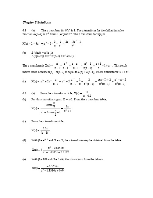
The difference equation can be found in two ways. By replacing h[n] with y[n] and [n] with x[n], the impulse response itself furnishes the difference equation y[n] = 2x[n] – 1.5x[n–1] + x[n–2] + 0.5x[n–3] Alternatively, the same difference equation can be found by using H(z) = Y(z)/X(z), cross-multiplying, and taking an inverse z transform. 6.9 n h[n] The samples of the impulse response are given in the table. 0 0.0 1 0.5625 2 0.3164 3 0.1780 4 0.0
The samples of the impulse responses are: 0 1.0 0.0 1 0.2 –3.0 2 0.04 –6.0 3 0.0 –9.0
The transfer functions of the systems are: H1(z) = 1 + 0.2z–1 + 0.04z–2 H2(z) = –3z–1 – 6z–2 – 9z–3 In cascade, the filters give the transfer function H(z) = H1(z)H2(z) = 3z 1 6.6z 2 10.32z 3 2.04z 4 0.36z 5 6.12 (b) 6.13 6.14
数字信号处理_Lecture 6

n = −∞
∑
∞
a n R N (n) z −n
n=0
∑
N
( az
−1
)n
1 − ( az − 1 ) N = 1 − az − 1
1 z N −1
zN − aN z − a
电子信息工程教研室
34
例题3-5
∑ ROC由满足n = 0
N
| az
电子信息工程教研室
30
例题3-4
X (z) =
n = −∞
∑ x(n ) z
∞
−n
=
n = −∞
∑ (−b z
n
−1
−n
)+
n=0
a n z −n ∑
∞
z z 1 1 = + = + −1 −1 z−b z−a 1 − bz 1 − az z(2 z − a − b) = ( z − a )( z − b )
n =0 +∞
ROC: Rx − < | z | ≤ ∞
(3-7)
因果序列的特征是:在|z|=∞ 处Z变换X(z)收敛。 Z
电子信息工程教研室
14
3.1.4 左边序列的Z变换 左边序列的Z
当n≤n2时,x(n)有非零值,而n> n2时,x(n)=0, 即左边序列。
X(z) = ∑x(n) z = ∑x(n) z +∑x(n) z(3-8)
X (z) = Z[x(n)] = a u(n)z = ∑a z = ∑(az−1)n ∑
n n=0 n=0 ∞ −n ∞ n −n ∞
n=−∞
这也是一个无穷项的等比级数求和,为了使X(z) 收敛,必须要求|az −1|<1,由此得到X(z)闭合
z变换信号流 -回复
z变换信号流-回复什么是z变换信号流?在数字信号处理中,z变换(Z-transform)是一种将离散时间信号转换为连续频域表示的数学工具。
z变换可以看作是拉普拉斯变换在离散时间中的对应物。
与傅里叶变换不同,z变换允许对非周期序列进行分析。
信号流是一个由离散时间的信号序列组成的流,其中每个时间点都有一个对应的采样值。
z变换信号流是在离散时间下对信号流进行z变换的过程。
通过对信号流进行z变换,我们可以在频域中对信号进行分析和处理。
下面,我将一步一步回答关于z变换信号流的问题,以帮助您更好地理解这个概念。
第一步:理解z变换的定义和基本概念在进行z变换之前,我们需要了解一些关于z变换的基本概念。
z变换将离散时间序列映射到连续复平面上的函数。
它的定义如下:X(z) = Σ[x(n) * z^(-n)]其中,x(n)是离散时间信号的序列,X(z)是z变换后的函数,n是时间索引。
这个公式表示了在离散时间序列x(n)的所有时刻n上对z的幂乘法之和。
第二步:了解z域和频域之间的关系在进行z变换时,我们将信号从时间域转换为z域。
z域是一个复平面,其中z从原点出发沿着虚轴旋转。
z的位置和幅度表示了信号的频率和幅度。
根据z变换的定义,我们可以将z域中的运算转换为频域中的运算。
第三步:计算信号流的z变换对于一个信号流,我们可以通过将其每个时间点的采样值带入到z变换的定义中,来计算其z变换。
即对于信号流x(n),计算其z变换X(z)的过程如下:1. 对于每个时间点n,将该点的采样值x(n)与z的幂乘法相乘。
2. 对所有时间点n上的乘积求和,得到z变换X(z)。
例如,对于信号流x(n) = {1, 2, 3, 4, 5},它的z变换可以计算如下:X(z) = 1*z^(-0) + 2*z^(-1) + 3*z^(-2) + 4*z^(-3) + 5*z^(-4)第四步:应用z变换信号流z变换信号流具有广泛的应用,特别是在数字信号处理中。
数字信号处理-z变换(new1)

z n1 1 z 4)(z 4
数字信号处理-第二章z变换与离散时间傅立叶变换(DTFT)
(1)
n 1 1 n 1 , X ( z ) z 在收敛域中作围线c, 当 在围线内有一个一阶极点 z 1 4 n 1 z 当 n 2, X ( z ) z 围线内有一个一阶极点 4 和一个高阶极点 z 0 n 1 1 故此时改求围线外留数。 j Im z 4 n 1, x(n) Re s[ X ( z ) z n 1 ] 1 z 1 4 ( 4) 4 4 ( n 1) 4n 4 , n 1 C 15 15 n 2, x(n) Re s[ X ( z ) z n 1 ]z 4 1/4 4
零点
z 0, z
有三种收敛域:
1 左边序列 2 1 2 ( 2) z 双边序列 2 3 (1) z
3 3 2 2 1 , z 极点z j , z j , z 4 4 3 3 2
2 (3) z 3
右边序列
数字信号处理-第二章z变换与离散时间傅立叶变换(DTFT)
例如:
5 2 z 1 1 n z x1 (n) u ( n 5) z 2 z 1 2z 2 n 2 n 5 1 0 z 2 n n n 5 5 2 z 1 1 n z x2 (n) u ( n 5) z 2 z 1 2z 2 n 2 n 5 1 0 z 2 n n n 5
j Im z
n 1, x(n) Re s[ X ( z ) z n 1 ]
n 1
z
1 4
Re s[ X ( z ) z n 1 ] z 4
数字信号处理基础-Z变换

(3) ZT[δ (n +1)] = ∑δ (n +1)z−n + ∑δ (n +1)z−n
n=−∞ n=0
> 0 z ≠ 0 > 0 z = 0, ) < 0 < 0, z z≠ ≠ )∞ −1 0
∞
= z1 + 0 = z (0 ≤ z < ∞)
光机电一体化技术研究所
ZT [u ( n )] = ∑ u ( n ) z
k k k →∞ −1
< 1或 z < 2
z < lim 2 = 2
k k k →∞
第二项仅含有Z的负幂的无穷级数 1 −k lim k ( z ) < 1或 z > lim k k →∞ k →∞ 3
k
∴ F ( z )的绝对收敛域为 2 > z >
光机电一体化技术研究所
1 3
光机电一体化技术研究所
×
1 Rx1 = 3
1
Re[z ]
3
1 (2) x(n) = − u (−n − 1) 3
1 −1 X ( z) = − ∑ z n = −∞ 3
−1 n n=− m ∞ −m
n
左边序列
1 −1 = − ∑ z m =1 3 ∞ 1 z m j Im[z ] = 1 − ∑ (3 z ) = 1 − = −1 1 1 − 3z m=0 z− Rx2 3 Re[z ] lim n (3 z ) n < 1 • ×
1
2
3
4
n
光机电一体化技术研究所
Z变换定义,典型序列的Z变换 变换定义,典型序列的 变换 变换定义
数字信号处理(英文版)课后习题答案2
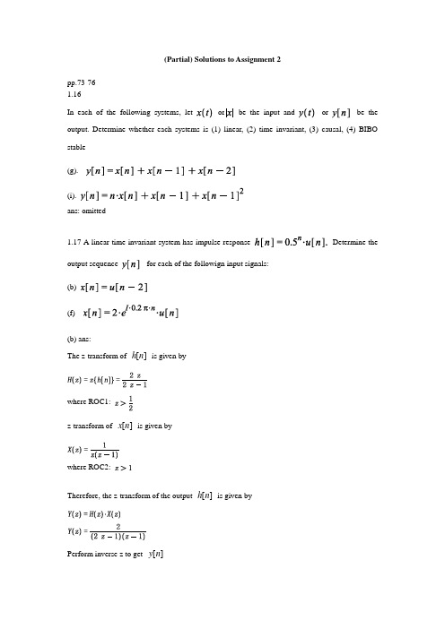
(Partial) Solutions to Assignment 2pp.73-761.16In each of the following systems, let or be the input and or be the output. Determine whether each systems is (1) linear, (2) time invariant, (3) causal, (4) BIBO stable(g).(i).ans: omitted----------------------------------------------------1.17 A linear time invariant system has impulse response Determine the output sequence for each of the followign input signals:(b)(f)(b) ans:h n is given byThe z-transform of []where ROC1:x n is given byz-transform of []where ROC2:h n is given byTherefore, the z-transform of the output []y nPerform inverse z to get [](f) ans: using the same method as in (b) (details omitted )----------------------------------------------------1.18. A linear time invariant system is defined by the difference equationb. Determine the output of the system when the intpu isc. Determine the output of the system when the input isans: omitted----------------------------------------------------1.19 The following expressions define linear time invariant systems. For each one determine the impulse respnose(a)(e)(a) ans: the impulse response is(e) ans: the impulse response is----------------------------------------------------1.20 Each of the following expressions defines a linear time invariant system. For each one determine whether it is BIBO stable or not(g)(k)BIBO: Bounded input and bounded output(g) ans: omitted(k) ans: omitted----------------------------------------------------1.21. Using the geometric series, for each of the following sequence determine the z-transform and its ROC(d)(g)(i)(d) ans:where ROC:(g) ans:The first part is equal towhere ROC1 isThe second part is equal towhere ROC2 isTherefore combining both parts:where ROC={ROC1 and ROC2}:(i) ans:where ROC: whole complex domain----------------------------------------------------1.22. You know what the and are. Using theproperties only (do not reuse the definition of the z-transform.) determine the z-transform of the following signals(c)(g)where ROC1:where ROC2:(c) ans: using z-transform property:We have:where ROC:(g) ans:details omitted. The final answer isTherefore combining both parts:where ROC={ROC1 and ROC2}:----------------------------------------------------1.23 Using partial fraction expansion, determine the inverse z-transform of the following functions:(c) ,(e) ,(c) ans:(e) ans:procedures are the same as above. details omitted.----------------------------------------------------1.24. For each of the followign linear difference equations, determine the impulse response, and indicate whether the system is BIBO stable or not(a)(c)(a) ans:Take z-transform on both sideswhere ROC:Because is finiteTherefore, the system is BIBO stable(c) ans: omitted (the same as (a))----------------------------------------------------1.25. Although most of the time we assume causality, a linear difference equation can be interpreted in a number of ways. Consider the linear difference equation(a) Determine the transfer function and the impulse response. Is the system causal ? BIBO stable ?(a) omitted.----------------------------------------------------1.26. 1.26 Consider the linear difference equation(a) Determine the transfer function . Do you have enough information to determine theregion of convergenceans:Don't have enough information to determine ROC.----------------------------------------------------1.27. Given the system described by the linear difference equationDetermine the output for each of the following input signals(a)(e)(a) ans:Take z-transform on both sides:----------------------------------------------------1.28. Repeat Problem 1.27 when the system is given in terms of the impulse responseBefore you do anything, is the system stable ? Does the frequency responseexist ?ans: omitted.----------------------------------------------------1.29. Repeat Problem 1.27 when the system isgiven by the linear difference equationBefore you do anything, is the system stable ? Does the frequency response exist ?Ans: omitted.----------------------------------------------------。
数字信号处理双语-Z变换.
6
• The set R of values of z for which its z-transform converges is called the Region Of Convergence (ROC)收敛域.
• X(z) converges if and only if
x[k]zk M
• H(z) is called as the transfer function传递函数 of system.
5ቤተ መጻሕፍቲ ባይዱ
Z transform of sequence
• For a given sequence x[n], its z-transform is
defined as
X (z) Z{x[n]} x[n]zn
3.5 Summary
1
Homework
• pp. 127-131 • 3.1 b f g • 3.2 • 3.6 b c
• 3.8 • 3.19 b • 3.20 a
2
3.0 Introduction
• Advantages of Z transform – It suits for more sequence analysis than Fourier transform. For many cases, we could have Z transforms for sequences when their Fourier transfroms do not exsist. – It is more convenient than Fourier transform in many analytical problem.
frequency, that is, z e jω , then
数字信号处理3第二章Z变换(OK)
(4)双边序列 可看做左边序列+右边序列,故其Z 可看做左边序列+右边序列,故其Z变换收敛域 应是这两个序列Z变换的公共收敛区间。 应是这两个序列Z变换的公共收敛区间。 Z变换
X ( z) =
n = −∞
∑ x( n) z
∞
−n
=
n = −∞
∑ x(n) z
−1
−n
+ ∑ x ( n) z
n =0
−1 n
X ( z) = ∑ a z
n =0
=∑ ( az )
n =0
1 z = = , −1 1 − az z−a
| z |>| a |
(3)左边序列 仅在n n 序列有值, 仅在n≤n2时,序列有值,n> n2时值全为零
x(n) x(n) = 0 Z变换为
X ( z) =
n = −∞
若X(z)只有一阶极点,X(z)展成 X(z)只有一阶极点,X(z)展成 只有一阶极点 k Am z X ( z ) = A0 + ∑ m =1 z − zm 最好写成
X ( z ) A0 k Am = +∑ z z m =1 z − zm
分别为X(z) z=0、 X(z)在 极点处的留数 A0、Am分别为X(z)在z=0、z=zm极点处的留数 X ( z) A0 = Re s[ , 0] = X ( 0) z X ( z) X ( z) Am = Re s[ , z m ] = [( z − z m ) ]z = zm z z
0 <| z |≤ ∞, 0 ≤| z |< ∞,
n1 ≥ 0 n2 ≤ 0
ROC 0 Re[z]
有限长序列的收敛域
(n), 例1:矩形序列是有限长序列,x(n)=RN(n), 矩形序列是有限长序列, 求其X(z) 求其X(z) 解: −N N −1 ∞
- 1、下载文档前请自行甄别文档内容的完整性,平台不提供额外的编辑、内容补充、找答案等附加服务。
- 2、"仅部分预览"的文档,不可在线预览部分如存在完整性等问题,可反馈申请退款(可完整预览的文档不适用该条件!)。
- 3、如文档侵犯您的权益,请联系客服反馈,我们会尽快为您处理(人工客服工作时间:9:00-18:30)。
M
∑∑ X ( z) =
P(z) Q(z)
=
bk z − k
k =0
N
ak z−k
k =0
(3.37)
Obtain an alternative expression for X(z) as a sum of simpler terms, each of which is tabulated.
The inverse z-transforms of each simple term is identified (from table 3.1) and summarized to get the desirable result x[n].
ROC of H(z) includes the unit circle (|z|= 1)
Causality: h[n] = 0, n < 0 (2.70) right-sided
ROC of H(z) : max{ pk } < z ≤ ∞
Stable and Causal:
ROC of H(z) : max{ pk }< z ≤ ∞, max{ pk }<1
Methods of determining the inverse z-transform z Inspection method z Partial fraction expansion z Power series expansion
15
3.3.1 Inspection method
The z-transform pairs in table 3.1 are invaluable in applying the inspection method
pi < z < p j ( pi < p j )
11
Stability, Causality and the ROC
H (z) = Z{h[n]} —— System Function
∞
Stability: ∑ h[n] < ∞ (2.65) n=−∞
The FT of h[n] exists.
09:06:41
Ch3. The z-transform
3.0 Introduction
z-transform for D-T signals
Laplace transform for C-T signals
The Fourier transform does not converge for all sequences, so it is useful to have a generalization of it.
7
ROC of Finite-duration sequences
x[n]
=
⎧≠ ⎨⎩=
0, 0,
N1 ≤ n ≤ N otherwise
2
N2
∑ X (z) = x[n]z−n n= N1
X(z) 是有限项级数和,只要级数的每一项有界,级 数就收敛,即要求:x[n] z −n < ∞ 由于x[n]有界,故要求:z −n < ∞
(3.8)
ROC: 0 ≤ Rg − < z < Rg + ≤ ∞
Rg + Rg −
5
Rational z-transform
X(z) is a rational function inside the ROC X (z) = P(z) Q(z)
zeros: the values of z for X(z)=0 poles: the values of z for X(z)=∞ The poles for finite values of z are the roots of Q(z). Poles may occur at z=0 or z=∞ . Important relationships exist between the locations
n=−∞
n= N1
n=−∞
正幂级数
0< z <∞
阿贝尔定理:存在一个收敛半径R,级数在以 原点为中心,以R为半径的圆内都绝对收敛。
0≤ z <R
0 < z < R ROC不能包含极点 0 < z < m in{ pk }
0≤
z
< min{ pk
}, N2
≤0 10
ROC of Two-sided sequences
An infinite-duration sequence extending from n = – ∞ to n = + ∞
two-sided sequence= right-sided sequence + left-sided sequence pi = max{ pRk } < z < ∞ 0 < z < min{ pLk } = pj
显然|z|在整个开域(0, ∞)都能满足以上条件,因此, 有限长序列的收敛域至少是除0和∞两个点以外的整 个z平面: 0 < z < ∞
若对N1, N2加以限制,收敛域可进一步扩大为包括0
点或∞点的半开域:
⎪⎧ 0 < ⎨⎪⎩0 ≤
z z
≤ ∞, N1 < ∞, N2
≥0 ≤0
8
ROC of Right-sided sequences
12
2
09:06:41
Example 3.7
ROC: 1 < z < 2 2
—— The system is stable.
ROC: z > 2 —— The system is causal.
ROC: z < 1 2
—— The system is neither stable nor causal. For this specfic pole-zero plot, there is no ROC that
(3.39)
If M≥N, and the poles are all first order,
∑ ∑ X
(z)
=
M −N r=0
Br
z−r
+
N k =1
1−
Ak dk
z−1
(3.43)
Br ——Long division Ak = (1− dk z−1)X(z) z=dk (3.41)
3.3.2 Partial fraction expansion
R< z ≤∞
X(z)的极点
R < z < ∞ ROC不能包含极点
max{ pk } < z < ∞
max{
pk
}<
z
≤ ∞,
N1
≥0 9
ROC of Left-sided sequences
x[n]
=
⎧≠ ⎨⎩ =
0, 0,
n n
≤ >
N2 N2
N2
N2
N1 −1
∑ ∑ ∑ X (z) = x[n]z−n = x[n]z−n + x[n]z−n (N1 ≤ 0)
3.3.2 Partial fraction expansion
M
∏ X ( z ) = b0 ∏ a 0
(1 − ck z −1 )
k =1
N
(1 − d k z −1 )
k =1
(3.39)
If M<N, and the poles are all first order,
∑ X
(z)
=
N
k =1 1 −
For any given sequence, the set of values of z for which the ZT converges, is call the region of convergence (ROC).
ZT convergence condition:
∞
∑ X (z) = x[n] z −n < ∞ n = −∞
x[n]
=
⎧≠
⎨ ⎩
=
0, 0,
n n
≥ <
N1 N1
j Im(z)
z-plane
a b c Re (z)
∞
N2
∞
∑ ∑ ∑ X (z) = x[n]z−n = x[n]z−n +
x[n]z−n (N2 ≥ 0)
n = N1
n = N1
n=N2 +1
负幂级数
0< z <∞
阿贝尔定理:存在一个收敛半径R,级数在以 原点为中心,以R为半径的圆外都绝对收敛。
of poles and the ROC. p104, table 3.1: Some common z-transform pairs
6
1
09:06:41
3.2 Properties of Region of Convergence
The ROC is a ring or disk in the z-plane centered at the origin: 0 ≤ Rg− < z < Rg+ ≤ ∞
would imply the system is both stable and causal. 13
Importance of ROC
ROC of ZT is an important concept. Without the knowledge of the ROC, there is no
n = −∞ ∞