The second phase transition in the pyrochlore oxide Cd2Re2O7
英语
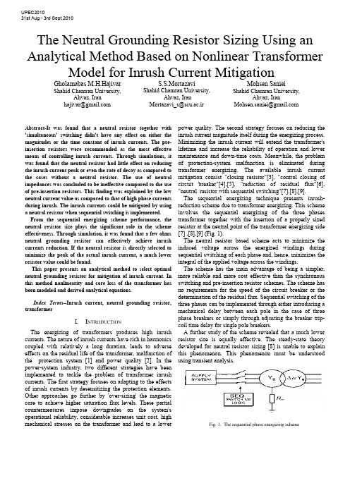
The Neutral Grounding Resistor Sizing Using an Analytical Method Based on Nonlinear Transformer Model for Inrush Current MitigationGholamabas M.H.Hajivar Shahid Chamran University,Ahvaz, Iranhajivar@S.S.MortazaviShahid Chamran University,Ahvaz, IranMortazavi_s@scu.ac.irMohsen SanieiShahid Chamran University,Ahvaz, IranMohsen.saniei@Abstract-It was found that a neutral resistor together with 'simultaneous' switching didn't have any effect on either the magnitudes or the time constant of inrush currents. The pre-insertion resistors were recommended as the most effective means of controlling inrush currents. Through simulations, it was found that the neutral resistor had little effect on reducing the inrush current peak or even the rate of decay as compared to the cases without a neutral resistor. The use of neutral impedances was concluded to be ineffective compared to the use of pre-insertion resistors. This finding was explained by the low neutral current value as compared to that of high phase currents during inrush. The inrush currents could be mitigated by using a neutral resistor when sequential switching is implemented. From the sequential energizing scheme performance, the neutral resistor size plays the significant role in the scheme effectiveness. Through simulation, it was found that a few ohms neutral grounding resistor can effectively achieve inrush currents reduction. If the neutral resistor is directly selected to minimize the peak of the actual inrush current, a much lower resistor value could be found.This paper presents an analytical method to select optimal neutral grounding resistor for mitigation of inrush current. In this method nonlinearity and core loss of the transformer has been modeled and derived analytical equations.Index Terms--Inrush current, neutral grounding resistor, transformerI.I NTRODUCTIONThe energizing of transformers produces high inrush currents. The nature of inrush currents have rich in harmonics coupled with relatively a long duration, leads to adverse effects on the residual life of the transformer, malfunction of the protection system [1] and power quality [2]. In the power-system industry, two different strategies have been implemented to tackle the problem of transformer inrush currents. The first strategy focuses on adapting to the effects of inrush currents by desensitizing the protection elements. Other approaches go further by 'over-sizing' the magnetic core to achieve higher saturation flux levels. These partial countermeasures impose downgrades on the system's operational reliability, considerable increases unit cost, high mechanical stresses on the transformer and lead to a lower power quality. The second strategy focuses on reducing the inrush current magnitude itself during the energizing process. Minimizing the inrush current will extend the transformer's lifetime and increase the reliability of operation and lower maintenance and down-time costs. Meanwhile, the problem of protection-system malfunction is eliminated during transformer energizing. The available inrush current mitigation consist "closing resistor"[3], "control closing of circuit breaker"[4],[5], "reduction of residual flux"[6], "neutral resistor with sequential switching"[7],[8],[9].The sequential energizing technique presents inrush-reduction scheme due to transformer energizing. This scheme involves the sequential energizing of the three phases transformer together with the insertion of a properly sized resistor at the neutral point of the transformer energizing side [7] ,[8],[9] (Fig. 1).The neutral resistor based scheme acts to minimize the induced voltage across the energized windings during sequential switching of each phase and, hence, minimizes the integral of the applied voltage across the windings.The scheme has the main advantage of being a simpler, more reliable and more cost effective than the synchronous switching and pre-insertion resistor schemes. The scheme has no requirements for the speed of the circuit breaker or the determination of the residual flux. Sequential switching of the three phases can be implemented through either introducing a mechanical delay between each pole in the case of three phase breakers or simply through adjusting the breaker trip-coil time delay for single pole breakers.A further study of the scheme revealed that a much lower resistor size is equally effective. The steady-state theory developed for neutral resistor sizing [8] is unable to explain this phenomenon. This phenomenon must be understood using transient analysis.Fig. 1. The sequential phase energizing schemeUPEC201031st Aug - 3rd Sept 2010The rise of neutral voltage is the main limitation of the scheme. Two methods present to control the neutral voltage rise: the use of surge arrestors and saturated reactors connected to the neutral point. The use of surge arresters was found to be more effective in overcoming the neutral voltage rise limitation [9].The main objective of this paper is to derive an analytical relationship between the peak of the inrush current and the size of the resistor. This paper presents a robust analytical study of the transformer energizing phenomenon. The results reveal a good deal of information on inrush currents and the characteristics of the sequential energizing scheme.II. SCHEME PERFORMANCESince the scheme adopts sequential switching, each switching stage can be investigated separately. For first-phase switching, the scheme's performance is straightforward. The neutral resistor is in series with the energized phase and this resistor's effect is similar to a pre-insertion resistor.The second- phase energizing is one of the most difficult to analyze. Fortunately, from simulation studies, it was found that the inrush current due to second-phase energizing is lower than that due to first-phase energizing for the same value of n R [9]. This result is true for the region where the inrush current of the first-phase is decreasing rapidly as n R increases. As a result, when developing a neutral-resistor-sizing criterion, the focus should be directed towards the analysis of the first-phase energizing.III. A NALYSIS OF F IRST -P HASE E NERGIZING The following analysis focuses on deriving an inrush current waveform expression covering both the unsaturatedand saturated modes of operation respectively. The presented analysis is based on a single saturated core element, but is suitable for analytical modelling of the single-phase transformers and for the single-phase switching of three-phase transformers. As shown in Fig. 2, the transformer's energized phase was modeled as a two segmented saturated magnetizing inductance in series with the transformer's winding resistance, leakage inductance and neutral resistance. The iron core non-l inear inductance as function of the operating flux linkages is represented as a linear inductor inunsaturated ‘‘m l ’’ and saturated ‘‘s l ’’ modes of operation respectively. (a)(b)Fig. 2. (a) Transformer electrical equivalent circuit (per-phase) referred to the primary side. (b) Simplified, two slope saturation curve.For the first-phase switching stage, the equivalent circuit represented in Fig. 2(a) can accurately represent behaviour of the transformer for any connection or core type by using only the positive sequence Flux-Current characteristics. Based on the transformer connection and core structure type, the phases are coupled either through the electrical circuit (3 single phase units in Yg-D connection) or through the Magnetic circuit (Core type transformers with Yg-Y connection) or through both, (the condition of Yg-D connection in an E-Core or a multi limb transformer). The coupling introduced between the windings will result in flux flowing through the limbs or magnetic circuits of un-energized phases. For the sequential switching application, the magnetic coupling will result in an increased reluctance (decreased reactance) for zero sequence flux path if present. The approach presented here is based on deriving an analytical expression relating the amount of inrush current reduction directly to the neutral resistor size. Investigation in this field has been done and some formulas were given to predict the general wave shape or the maximum peak current.A. Expression for magnitude of inrush currentIn Fig. 2(a), p r and p l present the total primary side resistance and leakage reactance. c R shows the total transformer core loss. Secondary side resistance sp r and leakage reactance sp l as referred to primary side are also shown. P V and s V represent the primary and secondary phase to ground terminal voltages, respectively.During first phase energizing, the differential equation describing behaviour of the transformer with saturated ironcore can be written as follows:()())sin((2) (1)φω+⋅⋅=⋅+⋅+⋅+=+⋅+⋅+=t V (t)V dtdi di d λdt di l (t)i R r (t)V dt d λdt di l (t)i R r (t)V m P ll p pp n p P p p p n p PAs the rate of change of the flux linkages with magnetizing current dt d /λcan be represented as an inductance equal to the slope of the i −λcurve, (2) can be re-written as follows;()(3) )()()(dtdi L dt di l t i R r t V lcore p p P n p P ⋅+⋅+⋅+=λ (4) )()(L core l p c l i i R dtdi−⋅=⋅λ⎩⎨⎧==sml core L L di d L λλ)(s s λλλλ>≤The general solution of the differential equations (3),(4) has the following form;⎪⎩⎪⎨⎧>−⋅⋅+−⋅+−−⋅+≤−⋅⋅+−⋅+−⋅=(5) )sin(//)()( )sin(//)(s s 22222221211112121111λλψωττλλψωττt B t e A t t e i A t B t e A t e A t i s s pSubscripts 11,12 and 21,22 denote un-saturated and saturated operation respectively. The parameters given in the equation (5) are given by;() )(/12221σ⋅++⎟⎟⎠⎞⎜⎜⎝⎛⋅−++⋅=m p c p m n p c m m x x R x x R r R x V B()2222)(/1σ⋅++⎟⎟⎠⎞⎜⎜⎝⎛⋅−++⋅=s p c p s n p c s m x x R x x R r R x V B⎟⎟⎟⎟⎟⎠⎞⎜⎜⎜⎜⎜⎝⎛⋅−+++=⋅−−⎟⎟⎟⎠⎞⎜⎜⎜⎝⎛−c p m n p m p c m R x x R r x x R x σφψ111tan tan ⎟⎟⎟⎟⎟⎠⎞⎜⎜⎜⎜⎜⎝⎛⋅−+++=⋅−−⎟⎟⎟⎠⎞⎜⎜⎜⎝⎛−c p s n p s p c m R R r x x R x σφψ112tan tan )sin(111211ψ⋅=+B A A )sin(222221s t B A A ⋅−⋅=+ωψ mp n p m p m p m p c xx R r x x x x x x R ⋅⋅+⋅−⋅+−⋅+⋅⋅⋅=)(4)()(21211σστm p n p m p m p m p c xx R r x x x x x x R ⋅⋅+⋅−⋅++⋅+⋅⋅⋅=)(4)()(21212σστ s p n p s p s p s p xx R r x x x x x x c R ⋅⋅+⋅−⋅+−⋅+⋅⋅⋅=)(4)()(21221σστ sp n p s p s p sp c xx R r x x x x x x R ⋅⋅+⋅−⋅++⋅+⋅⋅⋅=)(4)()(21222σστ ⎟⎟⎠⎞⎜⎜⎝⎛−⋅==s rs s ri i λλλ10 cnp R R r ++=1σ21221112 , ττττ>>>>⇒>>c R , 012≈A , 022≈A According to equation (5), the required inrush waveform assuming two-part segmented i −λcurve can be calculated for two separate un-saturated and saturated regions. For thefirst unsaturated mode, the current can be directly calculated from the first equation for all flux linkage values below the saturation level. After saturation is reached, the current waveform will follow the second given expression for fluxlinkage values above the saturation level. The saturation time s t can be found at the time when the current reaches the saturation current level s i .Where m λ,r λ,m V and ωare the nominal peak flux linkage, residual flux linkage, peak supply voltage and angular frequency, respectivelyThe inrush current waveform peak will essentially exist during saturation mode of operation. The focus should be concentrated on the second current waveform equation describing saturated operation mode, equation (5). The expression of inrush current peak could be directly evaluated when both saturation time s t and peak time of the inrush current waveform peak t t =are known [9].(10))( (9) )(2/)(222222121//)()(2B eA t e i A peak peak t s t s n peak n n peak R I R R t +−⋅+−−⋅+=+=ττωψπThe peak time peak t at which the inrush current will reachits peak can be numerically found through setting the derivative of equation (10) with respect to time equal to zero at peak t t =.()(11) )sin(/)(022222221212221/ψωωττττ−⋅⋅⋅−−−⋅+−=+−⋅peak t s t B A t te A i peak s peakeThe inrush waveform consists of exponentially decaying'DC' term and a sinusoidal 'AC' term. Both DC and AC amplitudes are significantly reduced with the increase of the available series impedance. The inrush waveform, neglecting the relatively small saturating current s i ,12A and 22A when extremely high could be normalized with respect to theamplitude of the sinusoidal term as follows; (12) )sin(/)()(2221221⎥⎦⎤⎢⎣⎡−⋅+−−⋅⋅=ψωτt t t e B A B t i s p(13) )sin(/)()sin()( 22221⎥⎦⎤⎢⎣⎡−⋅+−−⋅⋅−⋅=ψωτωψt t t e t B t i s s p ))(sin()( 2s n n t R R K ⋅−=ωψ (14) ωλλλφλφωλλφωmm m r s s t r m s mV t dt t V dtd t V V s=⎪⎭⎪⎬⎫⎪⎩⎪⎨⎧⎥⎥⎦⎤⎢⎢⎣⎡⎟⎟⎠⎞⎜⎜⎝⎛−−+−⋅=+⋅+⋅⋅==+⋅⋅=−∫(8) 1cos 1(7))sin((6))sin(10The factor )(n R K depends on transformer saturation characteristics (s λand r λ) and other parameters during saturation.Typical saturation and residual flux magnitudes for power transformers are in the range[9]; .).(35.1.).(2.1u p u p s <<λ and .).(9.0.).(7.0u p r u p <<λIt can be easily shown that with increased damping 'resistance' in the circuit, where the circuit phase angle 2ψhas lower values than the saturation angle s t ⋅ω, the exponential term is negative resulting in an inrush magnitude that is lowerthan the sinusoidal term amplitude.B. Neutral Grounding Resistor SizingBased on (10), the inrush current peak expression, it is now possible to select a neutral resistor size that can achieve a specific inrush current reduction ratio )(n R α given by:(15) )0(/)()(==n peak n peak n R I R I R α For the maximum inrush current condition (0=n R ), the total energized phase system impedance ratio X/R is high and accordingly, the damping of the exponential term in equation (10) during the first cycle can be neglected; [][](16))0(1)0()0(2212=⋅++⎥⎦⎤⎢⎣⎡⋅−+===⎟⎟⎠⎞⎜⎜⎝⎛+⋅⋅n s p c p s pR x n m n peak R x x R x x r R K V R I c s σ High n R values leading to considerable inrush current reduction will result in low X / R ratios. It is clear from (14) that X / R ratios equal to or less than 1 ensure negative DC component factor ')(n R K ' and hence the exponential term shown in (10) can be conservatively neglected. Accordingly, (10) can be re-written as follows;()[](17) )()(22122n s p c p s n p R x m n n peak R x x R x x R r V R B R I c s σ⋅++⎥⎦⎤⎢⎣⎡⋅−+=≈⎟⎟⎠⎞⎜⎜⎝⎛+⋅Using (16) and (17) to evaluate (15), the neutral resistorsize which corresponds to a specific reduction ratio can be given by;[][][](18) )0()(1)0( 12222=⋅++⋅−⋅++⋅−+⋅+=⎥⎥⎦⎤⎢⎢⎣⎡⎥⎥⎦⎤⎢⎢⎣⎡=n s p c p s p n s p c p s n p n R x x R x x r R x x R x x R r R K σσα Very high c R values leading to low transformer core loss, it can be re-written equation (18) as follows [9]; [][][][](19) 1)0(12222s p p s p n p n x x r x x R r R K +++++⋅+==α Equations (18) and (19) reveal that transformers require higher neutral resistor value to achieve the desired inrush current reduction rate. IV. A NALYSIS OF SECOND-P HASE E NERGIZING It is obvious that the analysis of the electric and magnetic circuit behavior during second phase switching will be sufficiently more complex than that for first phase switching.Transformer behaviour during second phase switching was served to vary with respect to connection and core structure type. However, a general behaviour trend exists within lowneutral resistor values where the scheme can effectively limitinrush current magnitude. For cases with delta winding or multi-limb core structure, the second phase inrush current is lower than that during first phase switching. Single phase units connected in star/star have a different performance as both first and second stage inrush currents has almost the same magnitude until a maximum reduction rate of about80% is achieved. V. NEUTRAL VOLTAGE RISEThe peak neutral voltage will reach values up to peak phasevoltage where the neutral resistor value is increased. Typicalneutral voltage peak profile against neutral resistor size is shown in Fig. 6- Fig. 8, for the 225 KVA transformer during 1st and 2nd phase switching. A del ay of 40 (ms) between each switching stage has been considered. VI. S IMULATION A 225 KVA, 2400V/600V, 50 Hz three phase transformer connected in star-star are used for the simulation study. The number of turns per phase primary (2400V) winding is 128=P N and )(01.0pu R R s P ==, )(05.0pu X X s P ==,active power losses in iron core=4.5 KW, average length and section of core limbs (L1=1.3462(m), A1=0.01155192)(2m ), average length and section of yokes (L2=0.5334(m),A2=0.01155192)(2m ), average length and section of air pathfor zero sequence flux return (L0=0.0127(m),A0=0.01155192)(2m ), three phase voltage for fluxinitialization=1 (pu) and B-H characteristic of iron core is inaccordance with Fig.3. A MATLAB program was prepared for the simulation study. Simulation results are shown in Fig.4-Fig.8.Fig. 3.B-H characteristic iron coreFig.4. Inrush current )(0Ω=n RFig.5. Inrush current )(5Ω=n RFig.6. Inrush current )(50Ω=n RFig.7. Maximum neutral voltage )(50Ω=n RFig.8. Maximum neutral voltage ).(5Ω=n RFig.9. Maximum inrush current in (pu), Maximum neutral voltage in (pu), Duration of the inrush current in (s)VII. ConclusionsIn this paper, Based on the sequential switching, presents an analytical method to select optimal neutral grounding resistor for transformer inrush current mitigation. In this method, complete transformer model, including core loss and nonlinearity core specification, has been used. It was shown that high reduction in inrush currents among the three phases can be achieved by using a neutral resistor .Other work presented in this paper also addressed the scheme's main practical limitation: the permissible rise of neutral voltage.VIII.R EFERENCES[1] Hanli Weng, Xiangning Lin "Studies on the UnusualMaloperation of Transformer Differential Protection During the Nonlinear Load Switch-In",IEEE Transaction on Power Delivery, vol. 24, no.4, october 2009.[2] Westinghouse Electric Corporation, Electric Transmissionand Distribution Reference Book, 4th ed. East Pittsburgh, PA, 1964.[3] K.P.Basu, Stella Morris"Reduction of Magnetizing inrushcurrent in traction transformer", DRPT2008 6-9 April 2008 Nanjing China.[4] J.H.Brunke, K.J.Frohlich “Elimination of TransformerInrush Currents by Controlled Switching-Part I: Theoretical Considerations” IEEE Trans. On Power Delivery, Vol.16,No.2,2001. [5] R. Apolonio,J.C.de Oliveira,H.S.Bronzeado,A.B.deVasconcellos,"Transformer Controlled Switching:a strategy proposal and laboratory validation",IEEE 2004, 11th International Conference on Harmonics and Quality of Power.[6] E. Andersen, S. Bereneryd and S. Lindahl, "SynchronousEnergizing of Shunt Reactors and Shunt Capacitors," OGRE paper 13-12, pp 1-6, September 1988.[7] Y. Cui, S. G. Abdulsalam, S. Chen, and W. Xu, “Asequential phase energizing method for transformer inrush current reduction—part I: Simulation and experimental results,” IEEE Trans. Power Del., vol. 20, no. 2, pt. 1, pp. 943–949, Apr. 2005.[8] W. Xu, S. G. Abdulsalam, Y. Cui, S. Liu, and X. Liu, “Asequential phase energizing method for transformer inrush current reduction—part II: Theoretical analysis and design guide,” IEEE Trans. Power Del., vol. 20, no. 2, pt. 1, pp. 950–957, Apr. 2005.[9] S.G. Abdulsalam and W. Xu "A Sequential PhaseEnergization Method for Transformer Inrush current Reduction-Transient Performance and Practical considerations", IEEE Transactions on Power Delivery,vol. 22, No.1, pp. 208-216,Jan. 2007.。
二维谱COSY

结束
rrernstswitzerlandrfreemanukoxford专业资料常见二维核磁的功能11hh11hhcosy22键或33键质子耦合11hh11hhtocsy具有连续的键合联系的质子耦合11hhxxhmqchsqc通过质子观察11键异核耦合11hhxxhmbc通过质子观察22或33键异核耦合多用于13ccxxxxcosy天然丰度大于20的杂核之间的11键耦合xxxxinadequate低天然丰度的杂核之间的11键耦合11hh11hhnoe差谱一维二维noesyroesy空间上接近质子之间的耦合专业资料常见二维核磁的功能专业资料二维核磁原理2dnmrisadomainofftandpulsedspectroscopy1d1d2d2ddetectsignalstwicebeforeaftercouplingsameas1dexperiment90?pulsetransfersbetweencoupledspins专业资料准备期preparation
Correlation Spectroscopy (COSY)--off-diagonal peaks
非对角线峰表明两种质子之间存在耦合。
Correlation Spectroscopy (COSY)--off-diagonal peaks
Correlation Spectroscopy (COSY)--off-diagonal peaks
6b 6a 5b
21b
Phase-Sensitive Spectra
Phase-Sensitive COSY
相敏COSY谱由于在数据处理中消除了通常与回波和反回波 相关的不需要的相扭曲线形和色散成分信号,只给出吸收 型信号,在提高灵敏度的同时,不但能够明显有效地改善 信号密集重叠区交叉峰的分辨率,而且提供了测定重叠区 内各信号化学位移和偶合常数的方法。
Chirality distribution and transition energies of carbon nanotubes

a r X i v :c o n d -m a t /0409220v 1 [c o n d -m a t .m t r l -s c i ] 9 S e p 2004Chirality distribution and transition energies of carbon nanotubesH.Telg,1J.Maultzsch,1S.Reich,2F.Hennrich,3and C.Thomsen 11Institut f¨u r Festk¨o rperphysik,Technische Universit¨a t Berlin,Hardenbergstr.36,10623Berlin,Germany2Department of Engineering,University of Cambridge,Cambridge CB21PZ,United Kingdom 3Institut f¨u r Nanotechnologie,Forschungszentrum Karlsruhe,76021Karlsruhe,Germany(Dated:February 2,2008)From resonant Raman scattering on isolated nanotubes we obtained the optical transition energies,the radial breathing mode frequency and Raman intensity of both metallic and semiconducting tubes.We unambiguously assigned the chiral index (n 1,n 2)of ≈50nanotubes based solely on a third-neighbor tight-binding Kataura plot and find ωRBM =(214.4±2)cm −1nm /d +(18.7±2)cm −1.In contrast to luminescence experiments we observe all chiralities including zig-zag tubes.The Raman intensities have a systematic chiral-angle dependence confirming recent ab-initio calculations.PACS numbers:78.67.Ch,73.22.-f,78.30.NaThe successful preparation of single-walled carbon nan-otubes in solution where the tubes are prevented from rebundling has opened a new direction in carbon nan-otube research [1,2,3,4].Strong luminescence by di-rect recombination from the band gap was detected in these isolated tubes,whereas in nanotube bundles no lu-minescence is observed.The electronic structure of car-bon nanotubes and the optical transition energies vary strongly with their chiral index (n 1,n 2)[5].Because the synthesis of nanotubes with a predefined chiral index has not been achieved so far,luminescence experiments were carried out on tube ensembles with unknown composition of chiral angles.Several attempts to assign the chiral in-dex (n 1,n 2)to the experimentally observed luminescence peaks were reported [2,4,6,7].With a unique assign-ment,one could validate and possibly revise theoretical models of the electronic band structure.Moreover,such an assignment would allow to characterize the tubes after their production and to control their separation [8].Bachilo et al.suggested an (n 1,n 2)assignment of the first and second transition energies in semiconducting tubes [2].Their assignment is based on pattern recogni-tion between experiment and theory in a plot of the sec-ond transition (excitation energy)versus the first transi-tion (emission energy)[9].The patterns,however,were not unique,and the frequency of the radial breathing mode (RBM)was used to find an anchoring element that singles out one of the assignments.Surprisingly,zig-zag tubes were not detected in these luminescence experi-ments.Bachilo et al.concluded that the concentration of tubes with chiral angles close to the zig-zag direction was very low in the sample [2].The electronic transition energies of metallic nan-otubes cannot be detected by luminescence experiments.An elegant approach is to record Raman resonance pro-files [10,11,12,13],with maximum intensity close to the real transitions in the electronic band structure.Reso-nance profiles from nanotubes in solution were first re-ported by Strano et al.[14];their (n 1,n 2)assignment to the transition energies was based on the RBM frequency to tube diameter relationship of Ref.[2].The resonance profiles of the so-assigned RBM peaks were then used to find an empirical expression for the transition energies in metallic tubes.In this paper we present the transition energies of both metallic and semiconducting nanotubes by reso-nant Raman spectroscopy.Plotting the resonance max-ima as a function of inverse RBM frequency,we obtain an (n 1,n 2)assignment without any additional assump-tions.From our assignment we fit c 1=214.4cm −1nm and c 2=18.7cm −1for the relation between diameter and RBM frequency.We observed several semiconduct-ing tubes that were not detectable by luminescence.Our results show that the electron-phonon coupling strength increases systematically for smaller chiral angles.Con-clusions about the distribution of chiral angles in a sam-ple based solely on luminescence intensity lead to incor-rect results;in particular,zig-zag tubes are present in nanotube ensembles.We performed Raman spectroscopy on HiPCO nan-otubes with diameters d ≈0.7−1.2nm [15].We dispersed the tubes in D 2O containing a surfactant,see Ref.[4]and used an Ar-Kr laser between 2.18and 2.62eV and two tunable lasers (1.85-2.15eV and 1.51-1.75eV).The spec-tra were collected with a Dilor XY800spectrometer in backscattering geometry at room temperature.To ob-tain the Raman cross section from the measured inten-sity we normalized the spectra to CaF 2and BaF 2mea-surements taken under the same experimental conditions (integration time,laser power).This also corrects for the spectrometer sensitivity and the ω4dependence of the Raman process.The Raman susceptibility was cal-culated from the normalized spectra by dividing by the Bose-Einstein occupation number and the inverse phonon frequency [16].The latter was omitted in Fig.1(a)for a better representation.In Fig.1(a)we show a contour plot of all Raman spectra,i.e.,the Raman scattering power as a function of inverse RBM frequency (1/ωRBM )and excitation en-ergy.When tuning the excitation energy,the RBM peaks23TABLE I:Measured ωRBM and E 22for thebranch ofthe(11,0)tube.See also supplementary material [17].chiral index(11,0)(10,2)(9,4)(8,6)n 21+n 1n 2+n 22/π,using a graphite lattice constant a 0=2.461˚A .c 1and c 2differ somewhat from the coefficients found in Ref.[2]for the same type of samples,because we used many more RBM frequencies for the fit and calculated the diameter from a smaller a 0.The coefficients are similar to theoret-ical predictions [18,19]but different from other experi-mental work [12,20].In Ref.[12],c 1and c 2were used as free parameters to find the assignment;moreover,the experimental information on the transition energies was not included.In Ref.[20],the chiral index assignment also depends on c 1(c 2=0).Moreover,the tubes are on a substrate,which might alter the RBM frequencies.In contrast,our assignment is not based on a choice for c 1and c 2.For the first time,they are obtained by a lin-ear fit after the assignment was performed.For example,the (11,0)tube has an RBM frequency of 266.7cm −1and E 22=1.657eV regardless of its exact diameter or any fit-ting procedure,see Table I.In addition to the semiconducting tubes,we directly obtained the transition energies of metallic tubes.Our assignment of the metallic tubes to RBM frequencies agrees well with Strano et al.[14].The empirically ob-tained transition energies in Ref.[14],however,underes-timate the experimental values in Fig.1(b).Moreover,our data show a stronger bending of the branches towards small chiral angles.This discrepancy comes mainly from the presence of pairs of close-by transition energies in chiral metallic tubes [21].This ambiguity led to an in-correct assignment of single data points to the upper or lower transition.Given the unique (n 1,n 2)assignment of the RBM and the resonance energies,we can now examine the chirality dependence of the transition energies and of the RBM intensity.The optical transition energies of carbon nan-otubes are roughly proportional to 1/d [9,21,22,23].Tight-binding calculations predict deviations from a pure 1/d dependence as a function of chiral angle [21].They lead to the branches in the Kataura plot and are more pronounced if third-nearest neighbors are included [9].Still,the band gap energies of tubes with small chiral angle (zig-zag tubes)are systematically lower in first-principles calculations than in zone folding [24].The branches in the experimental Kataura plot of Fig.1(b)are an experimental verification of the predictions from ab-initio calculations.The chiral-angle dependent softening of the transition energies with respect to the third-order tight-binding calculations is due to rehybridization of the πand σbands [9,24,25].It is stronger for the states originat-ing from between the K and M point of the graphite Brillouin zone in the zone-folding approach and weaker for states from the other side of the K point [24].In semiconducting tubes,the value of ν=(n 1−n 2)mod 3determines from which side of the K point the electronic states originate for a given optical transition.The tubes in the lower branches of the E 22transitions in semicon-ducting tubes,i.e.,of the branches beginning with (9,1),(11,0),and (12,1)in Fig.1(b),have ν=−1.The soft-ening for small-chiral-angle tubes in these branches com-pared to the tight-binding value is quite strong.The tubes in the upper part of the same set of transitions have ν=+1and are less affected by the softening.For example,the experimental transition energy of the (10,0)tube [θ=0◦,ν=+1]matches the theoretical value very well [Fig.1(b)].Taking this softening of the transition energies in the −1families into account,the agreement of our data with the theoretical predictions is excellent.In general,the RBM signal was strong for nanotubes with ν=−1and also from the lower branches of the metallic transitions in Fig.1(b).The intensities were by a factor of four to ten weaker for tubes with ν=+1.This observation confirms ab-initio calculations of the electron-phonon coupling that predicted the magnitude of the electron-phonon matrix element to alternate with4Chiral angle (deg.)I n t e n s i t y (a r b . u n i t s )FIG.2:(Color online)Raman intensity as a function of the chiral angle for three nanotube branches (solid circles)with (n 1,n 2)as indicated.Open circles:calculated Raman inten-sity,see text.(a)and (b)contain semiconducting,(c)contains metallic tubes.ν[26].The relative Raman intensity of the RBM can also be used to discriminate between the two families of semiconducting tubes.The assignment of the semiconducting tubes in Fig.1(b)corresponds to the one found by Bachilo et al.from luminescence experiments [2].In contrast to the luminescence results,which reported a maximum in-tensity for close-to-armchair tubes and no emission from zig-zag tubes,we clearly observed zig-zag or close-to-zig-zag tubes as well.The (13,0),(11,0),and the (10,0)tube show that zig-zag tubes are present in the sample.These tubes as well as the (14,1)tube were not observed by photoluminescence.An important conclusion from our work is that the absence of photoluminescence from these tubes thus does not imply the preferential growth of armchair tubes.In Fig.2we show the resonance maxima for tubes be-longing to the same (n 1−1,n 2+2)branch.The Raman intensity increases with decreasing chiral angle θand is at maximum for θ≈10−15◦,except for (a).Theoretically,the Raman amplitude is proportional to the electron-phonon coupling times the square of the optical absorp-tion strength [16].Mach´o n et al.[26]found that the electron-phonon coupling of the RBM decreases strongly with increasing θ.We therefore model the electron-phonon interaction by a linear function of the chiral angle with a three times stronger coupling for zig-zag than for armchair tubes as found in Ref.[26].We approximate the optical absorption strength of a tube by its experi-mental photoluminescence intensity [2],i.e.,we assume the absorption andemission probability to be the same.The relative Ra-man intensities calculated with this model are in good agreement with experiment (open dots in Fig.2).The Raman response of zig-zag tubes is enhanced compared to their luminescence intensity because of their strong electron-phonon coupling.On the other hand,the Ra-man intensity of zig-zag tubes is smaller than for θ≈10◦due to the small absorption coefficient.Thus,our data are completely consistent with a uniform chirality distri-bution in the sample.In conclusion,we assigned the chiral indices to ≈50measured RBM frequencies and transition energies by resonant Raman spectroscopy.In contrast to all pre-vious work our assignment is independent of the co-efficients c 1and c 2,which we fit only after assigning the chiral index to a particular RBM.The largest Ra-man intensity was measured for tubes with chiral angles around 15◦or smaller,which is in agreement with the-oretical predictions and implies that the chiralities are evenly distributed.Moreover,our results confirm that the RBM intensity in semiconducting tubes depends on the (n 1−n 2)mod 3family.The transition energies de-viate from zone-folding predictions with decreasing chi-ral angle,which,in particular for metallic tubes,was strongly underestimated in earlier work.This work was supported by the DFG under grant number Th662/8-2.S.R.was supported by the Oppen-heimer Fund and Newnham College.[1]M.J.O’Connell,et al.,Science 297,593(2002).[2]S.M.Bachilo,et al.,Science 298,2361(2002).[3]J.Lefebvre,et al.,Phys.Rev.Lett.90,217401(2003).[4]S.Lebedkin,et al.,J.Phys.Chem.B 107,1949(2003).[5]S.Reich,C.Thomsen,and J.Maultzsch,Carbon Nan-otubes:Basic Concepts and Physical Properties (Wiley-VCH,Berlin,2004).[6]A.Hagen and T.Hertel,Nano Lett.3,383(2003).[7]R.B.Weisman and S.M.Bachilo,Nano Lett.3,1235(2003).[8]R.Krupke,F.Hennrich,H.v.L¨o hneysen,and M.M.Kappes,Science 301,344(2003).[9]S.Reich,J.Maultzsch,C.Thomsen,and P.Ordej´o n,Phys.Rev.B 66,035412(2002).[10]A.Jorio,et al.,Phys.Rev.B 63,245416(2001).[11]M.Canonico,et al.,Phys.Rev.B 65,201402(R)(2002).[12]C.Kramberger,et al.,Phys.Rev.B 68,235404(2003).[13]S.K.Doorn,et al.,Appl.Phys.A 78,1147(2004).[14]M.S.Strano,et al.,Nano Lett.3,1091(2003).[15]P.Nikolaev,et al.,Chem.Phys.Lett.313,91(1999).[16]M.Cardona,in Light Scattering in Solids II ,edited by M.Cardona and G.G¨u ntherodt (Springer,Berlin,1982),vol.50of Topics in Applied Physics ,p.19.[17]See EPAPS Document No.[]for a table containing the complete branches of Fig.1(b).[18]J.K¨u rti,G.Kresse,and H.Kuzmany,Phys.Rev.B 58,8869(1998).[19]E.Dobardˇz i´c ,I.M.B.Nikoli´c ,T.Vukovi´c ,and M.Damn-janovi´c ,Phys.Rev.B 68,045408(2003).[20]A.Jorio,et al.,Phys.Rev.Lett.86,1118(2001).[21]S.Reich and C.Thomsen,Phys.Rev.B 62,4273(2000).[22]J.W.Mintmire and C.T.White,Phys.Rev.Lett.81,2506(1998).[23]H.Kataura,et al.,Synth.Met.103,2555(1999).[24]S.Reich,C.Thomsen,and P.Ordej´o n,Phys.Rev.B 65,155411(2002).[25]X.Blase,et al.,Phys.Rev.Lett.72,1878(1994).[26]M.Mach´o n,et al.,(2003),submitted to Phys.Rev.B;5 cond-mat/0408436v1.。
菲涅耳非相干关联全息图(综述)

Fresnel incoherent correlation hologram-a reviewInvited PaperJoseph Rosen,Barak Katz1,and Gary Brooker2∗∗1Department of Electrical and Computer Engineering,Ben-Gurion University of the Negev,P.O.Box653,Beer-Sheva84105,Israel2Johns Hopkins University Microscopy Center,Montgomery County Campus,Advanced Technology Laboratory, Whiting School of Engineering,9605Medical Center Drive Suite240,Rockville,MD20850,USA∗E-mail:rosen@ee.bgu.ac.il;∗∗e-mail:gbrooker@Received July17,2009Holographic imaging offers a reliable and fast method to capture the complete three-dimensional(3D) information of the scene from a single perspective.We review our recently proposed single-channel optical system for generating digital Fresnel holograms of3D real-existing objects illuminated by incoherent light.In this motionless holographic technique,light is reflected,or emitted from a3D object,propagates througha spatial light modulator(SLM),and is recorded by a digital camera.The SLM is used as a beam-splitter of the single-channel incoherent interferometer,such that each spherical beam originated from each object point is split into two spherical beams with two different curve radii.Incoherent sum of the entire interferences between all the couples of spherical beams creates the Fresnel hologram of the observed3D object.When this hologram is reconstructed in the computer,the3D properties of the object are revealed.OCIS codes:100.6640,210.4770,180.1790.doi:10.3788/COL20090712.0000.1.IntroductionHolography is an attractive imaging technique as it offers the ability to view a complete three-dimensional (3D)volume from one image.However,holography is not widely applied to the regime of white-light imaging, because white-light is incoherent and creating holograms requires a coherent interferometer system.In this review, we describe our recently invented method of acquiring incoherent digital holograms.The term incoherent digi-tal hologram means that incoherent light beams reflected or emitted from real-existing objects interfere with each other.The resulting interferogram is recorded by a dig-ital camera and digitally processed to yield a hologram. This hologram is reconstructed in the computer so that 3D images appear on the computer screen.The oldest methods of recording incoherent holograms have made use of the property that every incoherent ob-ject is composed of many source points,each of which is self-spatial coherent and can create an interference pattern with light coming from the point’s mirrored image.Under this general principle,there are vari-ous types of holograms[1−8],including Fourier[2,6]and Fresnel holograms[3,4,8].The process of beam interfering demands high levels of light intensity,extreme stability of the optical setup,and a relatively narrow bandwidth light source.More recently,three groups of researchers have proposed computing holograms of3D incoherently illuminated objects from a set of images taken from differ-ent points of view[9−12].This method,although it shows promising prospects,is relatively slow since it is based on capturing tens of scene images from different view angles. Another method is called scanning holography[13−15],in which a pattern of Fresnel zone plates(FZPs)scans the object such that at each and every scanning position, the light intensity is integrated by a point detector.The overall process yields a Fresnel hologram obtained as a correlation between the object and FZP patterns.How-ever,the scanning process is relatively slow and is done by mechanical movements.A similar correlation is ac-tually also discussed in this review,however,unlike the case of scanning holography,our proposed system carries out a correlation without movement.2.General properties of Fresnel hologramsThis review concentrates on the technique of incoher-ent digital holography based on single-channel incoher-ent interferometers,which we have been involved in their development recently[16−19].The type of hologram dis-cussed here is the digital Fresnel hologram,which means that a hologram of a single point has the form of the well-known FZP.The axial location of the object point is encoded by the Fresnel number of the FZP,which is the technical term for the number of the FZP rings along the given radius.To understand the operation principle of any general Fresnel hologram,let us look on the difference between regular imaging and holographic systems.In classical imaging,image formation of objects at different distances from the lens results in a sharp image at the image plane for objects at only one position from the lens,as shown in Fig.1(a).The other objects at different distances from the lens are out of focus.A Fresnel holographic system,on the other hand,as depicted in Fig.1(b),1671-7694/2009/120xxx-08c 2009Chinese Optics Lettersprojects a set of rings known as the FZP onto the plane of the image for each and every point at every plane of the object being viewed.The depth of the points is en-coded by the density of the rings such that points which are closer to the system project less dense rings than distant points.Because of this encoding method,the 3D information in the volume being imaged is recorded into the recording medium.Thus once the patterns are decoded,each plane in the image space reconstructed from a Fresnel hologram is in focus at a different axial distance.The encoding is accomplished by the presence of a holographic system in the image path.At this point it should be noted that this graphical description of pro-jecting FZPs by every object point actually expresses the mathematical two-dimensional (2D)correlation (or convolution)between the object function and the FZP.In other words,the methods of creating Fresnel holo-grams are different from each other by the way they spatially correlate the FZP with the scene.Another is-sue to note is that the correlation should be done with a FZP that is somehow “sensitive”to the axial locations of the object points.Otherwise,these locations are not encoded into the hologram.The system described in this review satisfies the condition that the FZP is depen-dent on the axial distance of each and every objectpoint.parison between the Fresnel holography principle and conventional imaging.(a)Conventional imaging system;(b)fresnel holographysystem.Fig.2.Schematic of FINCH recorder [16].BS:beam splitter;L is a spherical lens with focal length f =25cm;∆λindicates a chromatic filter with a bandwidth of ∆λ=60nm.This means that indeed points,which are closer to the system,project FZP with less cycles per radial length than distant points,and by this condition the holograms can actually image the 3D scene properly.The FZP is a sum of at least three main functions,i.e.,a constant bias,a quadratic phase function and its complex conjugate.The object function is actually corre-lated with all these three functions.However,the useful information,with which the holographic imaging is real-ized,is the correlation with just one of the two quadratic phase functions.The correlation with the other quadratic phase function induces the well-known twin image.This means that the detected signal in the holographic system contains three superposed correlation functions,whereas only one of them is the required correlation between the object and the quadratic phase function.Therefore,the digital processing of the detected image should contain the ability to eliminate the two unnecessary terms.To summarize,the definition of Fresnel hologram is any hologram that contains at least a correlation (or convolu-tion)between an object function and a quadratic phase function.Moreover,the quadratic phase function must be parameterized according to the axial distance of the object points from the detection plane.In other words,the number of cycles per radial distance of each quadratic phase function in the correlation is dependent on the z distance of each object point.In the case that the object is illuminated by a coherent wave,this correlation is the complex amplitude of the electromagnetic field directly obtained,under the paraxial approximation [20],by a free propagation from the object to the detection plane.How-ever,we deal here with incoherent illumination,for which an alternative method to the free propagation should be applied.In fact,in this review we describe such method to get the desired correlation with the quadratic phase function,and this method indeed operates under inco-herent illumination.The discussed incoherent digital hologram is dubbed Fresnel incoherent correlation hologram (FINCH)[16−18].The FINCH is actually based on a single-channel on-axis incoherent interferometer.Like any Fresnel holography,in the FINCH the object is correlated with a FZP,but the correlation is carried out without any movement and without multiplexing the image of the scene.Section 3reviews the latest developments of the FINCH in the field of color holography,microscopy,and imaging with a synthetic aperture.3.Fresnel incoherent correlation holographyIn this section we describe the FINCH –a method of recording digital Fresnel holograms under incoher-ent illumination.Various aspects of the FINCH have been described in Refs.[16-19],including FINCH of re-flected white light [16],FINCH of fluorescence objects [17],a FINCH-based holographic fluorescence microscope [18],and a hologram recorder in a mode of a synthetic aperture [19].We briefly review these works in the current section.Generally,in the FINCH system the reflected incoher-ent light from a 3D object propagates through a spatial light modulator (SLM)and is recorded by a digital cam-era.One of the FINCH systems [16]is shown in Fig.2.White-light source illuminates a 3D scene,and the reflected light from the objects is captured by a charge-coupled device (CCD)camera after passing through a lens L and the SLM.In general,we regard the system as an incoherent interferometer,where the grating displayed on the SLM is considered as a beam splitter.As is com-mon in such cases,we analyze the system by following its response to an input object of a single infinitesimal point.Knowing the system’s point spread function (PSF)en-ables one to realize the system operation for any general object.Analysis of a beam originated from a narrow-band infinitesimal point source is done by using Fresnel diffraction theory [20],since such a source is coherent by definition.A Fresnel hologram of a point object is obtained when the two interfering beams are two spherical beams with different curvatures.Such a goal is achieved if the SLM’s reflection function is a sum of,for instance,constant and quadratic phase functions.When a plane wave hits the SLM,the constant term represents the reflected plane wave,and the quadratic phase term is responsible for the reflected spherical wave.A point source located at some distance from a spher-ical positive lens induces on the lens plane a diverging spherical wave.This wave is split by the SLM into two different spherical waves which propagate toward the CCD at some distance from the SLM.Consequently,in the CCD plane,the intensity of the recorded hologram is a sum of three terms:two complex-conjugated quadratic phase functions and a constant term.This result is the PSF of the holographic recording system.For a general 3D object illuminated by a narrowband incoherent illumination,the intensity of the recorded hologram is an integral of the entire PSFs,over all object intensity points.Besides a constant term,thehologramFig.3.(a)Phase distribution of the reflection masks dis-played on the SLM,with θ=0◦,(b)θ=120◦,(c)θ=240◦.(d)Enlarged portion of (a)indicating that half (randomly chosen)of the SLM’s pixels modulate light with a constant phase.(e)Magnitude and (f)phase of the final on-axis digi-tal hologram.(g)Reconstruction of the hologram of the three characters at the best focus distance of ‘O’.(h)Same recon-struction at the best focus distance of ‘S’,and (i)of ‘A’[16].expression contains two terms of correlation between an object and a quadratic phase,z -dependent,function.In order to remain with a single correlation term out of the three terms,we follow the usual procedure of on-axis digital holography [14,16−19].Three holograms of the same object are recorded with different phase con-stants.The final hologram is a superposition of the three holograms containing only the desired correlation between the object function and a single z -dependent quadratic phase.A 3D image of the object can be re-constructed from the hologram by calculating theFresnelFig.4.Schematics of the FINCH color recorder [17].L 1,L 2,L 3are spherical lenses and F 1,F 2are chromaticfilters.Fig.5.(a)Magnitude and (b)phase of the complex Fres-nel hologram of the dice.Digital reconstruction of the non-fluorescence hologram:(c)at the face of the red dots on the die,and (d)at the face of the green dots on the die.(e)Magnitude and (f)phase of the complex Fresnel hologram of the red dots.Digital reconstruction of the red fluorescence hologram:(g)at the face of the red dots on the die,and (h)at the face of the green dots on the die.(i)Magnitude and (j)phase of the complex Fresnel hologram of the green dots.Digital reconstruction of the green fluorescence hologram:(k)at the face of the red dots on the die,and (l)at the face of the green dots on the position of (c),(g),(k)and that of (d),(h),(l)are depicted in (m)and (n),respectively [17].Fig.6.FINCHSCOPE schematic in uprightfluorescence microscope[18].propagation formula.The system shown in Fig.2has been used to record the three holograms[16].The SLM has been phase-only, and as so,the desired sum of two phase functions(which is no longer a pure phase)cannot be directly displayed on this SLM.To overcome this obstacle,the quadratic phase function has been displayed randomly on only half of the SLM pixels,and the constant phase has been displayed on the other half.The randomness in distributing the two phase functions has been required because organized non-random structure produces unnecessary diffraction orders,therefore,results in lower interference efficiency. The pixels are divided equally,half to each diffractive element,to create two wavefronts with equal energy.By this method,the SLM function becomes a good approx-imation to the sum of two phase functions.The phase distributions of the three reflection masks displayed on the SLM,with phase constants of0◦,120◦and240◦,are shown in Figs.3(a),(b)and(c),respectively.Three white-on-black characters i th the same size of 2×2(mm)were located at the vicinity of rear focal point of the lens.‘O’was at z=–24mm,‘S’was at z=–48 mm,and‘A’was at z=–72mm.These characters were illuminated by a mercury arc lamp.The three holo-grams,each for a different phase constant of the SLM, were recorded by a CCD camera and processed by a computer.Thefinal hologram was calculated accord-ing to the superposition formula[14]and its magnitude and phase distributions are depicted in Figs.3(e)and (f),respectively.The hologram was reconstructed in the computer by calculating the Fresnel propagation toward various z propagation distances.Three different recon-struction planes are shown in Figs.3(g),(h),and(i).In each plane,a different character is in focus as is indeed expected from a holographic reconstruction of an object with a volume.In Ref.[17],the FINCH has been capable to record multicolor digital holograms from objects emittingfluo-rescent light.Thefluorescent light,specific to the emis-sion wavelength of variousfluorescent dyes after excita-tion of3D objects,was recorded on a digital monochrome camera after reflection from the SLM.For each wave-length offluorescent emission,the camera sequentially records three holograms reflected from the SLM,each with a different phase factor of the SLM’s function.The three holograms are again superposed in the computer to create a complex-valued Fresnel hologram of eachflu-orescent emission without the twin image problem.The holograms for eachfluorescent color are further combined in a computer to produce a multicoloredfluorescence hologram and3D color image.An experiment showing the recording of a colorfluo-rescence hologram was carried out[17]on the system in Fig. 4.The phase constants of0◦,120◦,and240◦were introduced into the three quadratic phase functions.The magnitude and phase of thefinal complex hologram,su-perposed from thefirst three holograms,are shown in Figs.5(a)and(b),respectively.The reconstruction from thefinal hologram was calculated by using the Fresnel propagation formula[20].The results are shown at the plane of the front face of the front die(Fig.5(c))and the plane of the front face of the rear die(Fig.5(d)).Note that in each plane a different die face is in focus as is indeed expected from a holographic reconstruction of an object with a volume.The second three holograms were recorded via a redfilter in the emissionfilter slider F2 which passed614–640nmfluorescent light wavelengths with a peak wavelength of626nm and a full-width at half-maximum,of11nm(FWHM).The magnitude and phase of thefinal complex hologram,superposed from the‘red’set,are shown in Figs.5(e)and(f),respectively. The reconstruction results from thisfinal hologram are shown in Figs.5(g)and(h)at the same planes as those in Figs.5(c)and(d),respectively.Finally,an additional set of three holograms was recorded with a greenfilter in emissionfilter slider F2,which passed500–532nmfluo-rescent light wavelengths with a peak wavelength of516 nm and a FWHM of16nm.The magnitude and phase of thefinal complex hologram,superposed from the‘green’set,are shown in Figs.5(i)and(j),respectively.The reconstruction results from thisfinal hologram are shown in Figs.5(k)and(l)at the same planes as those in Fig. 5(c)and(d),positions of Figs.5(c), (g),and(k)and Figs.5(d),(h),and(l)are depicted in Figs.5(m)and(n),respectively.Note that all the colors in Fig.5(colorful online)are pseudo-colors.These last results yield a complete color3D holographic image of the object including the red and greenfluorescence. While the optical arrangement in this demonstration has not been optimized for maximum resolution,it is im-portant to recognize that even with this simple optical arrangement,the resolution is good enough to image the fluorescent emissions with goodfidelity and to obtain good reflected light images of the dice.Furthermore, in the reflected light images in Figs.5(c)and(m),the system has been able to detect a specular reflection of the illumination from the edge of the front dice. Another system to be reviewed here is thefirst demon-stration of a motionless microscopy system(FINCH-SCOPE)based upon the FINCH and its use in record-ing high-resolution3Dfluorescent images of biological specimens[18].By using high numerical aperture(NA) lenses,a SLM,a CCD camera,and some simplefilters, FINCHSCOPE enables the acquisition of3D microscopic images without the need for scanning.A schematic diagram of the FINCHSCOPE for an upright microscope equipped with an arc lamp sourceFig.7.FINCHSCOPE holography of polychromatic beads.(a)Magnitude of the complex hologram 6-µm beads.Images reconstructed from the hologram at z distances of (b)34µm,(c)36µm,and (d)84µm.Line intensity profiles between the beads are shown at the bottom of panels (b)–(d).(e)Line intensity profiles along the z axis for the lower bead from reconstructed sections of a single hologram (line 1)and from a widefield stack of the same bead (28sections,line 2).Beads (6µm)excited at 640,555,and 488nm with holograms reconstructed (f)–(h)at plane (b)and (j)–(l)at plane (d).(i)and (m)are the combined RGB images for planes (b)and (d),respectively.(n)–(r)Beads (0.5µm)imaged with a 1.4-NA oil immersion objective:(n)holographic camera image;(o)magnitude of the complex hologram;(p)–(r)reconstructed image at planes 6,15,and 20µm.Scale bars indicate image size [18].Fig.8.FINCHSCOPE fluorescence sections of pollen grains and Convallaria rhizom .The arrows point to the structures in the images that are in focus at various image planes.(b)–(e)Sections reconstructed from a hologram of mixed pollen grains.(g)–(j)Sections reconstructed from a hologram of Convallaria rhizom .(a),(f)Magnitudes of the complex holograms from which the respective image planes are reconstructed.Scale bars indicate image size [18].is shown in Fig. 6.The beam of light that emerges from an infinity-corrected microscope objective trans-forms each point of the object being viewed into a plane wave,thus satisfying the first requirement of FINCH [16].A SLM and a digital camera replace the tube lens,reflec-tive mirror,and other transfer optics normally present in microscopes.Because no tube lens is required,infinity-corrected objectives from any manufacturer can be used.A filter wheel was used to select excitation wavelengths from a mercury arc lamp,and the dichroic mirror holder and the emission filter in the microscope were used to direct light to and from the specimen through an infinity-corrected objective.The ability of the FINCHSCOPE to resolve multicolor fluorescent samples was evaluated by first imaging poly-chromatic fluorescent beads.A fluorescence bead slidewith the beads separated on two separate planes was con-structed.FocalCheck polychromatic beads(6µm)were used to coat one side of a glass microscope slide and a glass coverslip.These two surfaces were juxtaposed and held together at a distance from one another of∼50µm with optical cement.The beads were sequentially excited at488-,555-,and640-nm center wavelengths(10–30nm bandwidths)with emissions recorded at515–535,585–615,and660–720nm,respectively.Figures7(a)–(d) show reconstructed image planes from6µm beads ex-cited at640nm and imaged on the FINCHSCOPE with a Zeiss PlanApo20×,0.75NA objective.Figure7(a) shows the magnitude of the complex hologram,which contains all the information about the location and in-tensity of each bead at every plane in thefield.The Fresnel reconstruction from this hologram was selected to yield49planes of the image,2-µm apart.Two beads are shown in Fig.7(b)with only the lower bead exactly in focus.Figure7(c)is2µm into thefield in the z-direction,and the upper bead is now in focus,with the lower bead slightly out of focus.The focal difference is confirmed by the line profile drawn between the beads, showing an inversion of intensity for these two beads be-tween the planes.There is another bead between these two beads,but it does not appear in Figs.7(b)or(c) (or in the intensity profile),because it is48µm from the upper bead;it instead appears in Fig.7(d)(and in the line profile),which is24sections away from the section in Fig.7(c).Notice that the beads in Figs.7(b)and(c)are no longer visible in Fig.7(d).In the complex hologram in Fig.7(a),the small circles encode the close beads and the larger circles encode the distant central bead. Figure7(e)shows that the z-resolution of the lower bead in Fig.7(b),reconstructed from sections created from a single hologram(curve1),is at least comparable to data from a widefield stack of28sections(obtained by moving the microscope objective in the z-direction)of the same field(curve2).The co-localization of thefluorescence emission was confirmed at all excitation wavelengths and at extreme z limits,as shown in Figs.7(f)–(m)for the 6-µm beads at the planes shown in Figs.7(b)((f)–(i)) and(d)((j)–(m)).In Figs.7(n)–(r),0.5-µm beads imaged with a Zeiss PlanApo×631.4NA oil-immersion objective are shown.Figure7(n)presents one of the holo-grams captured by the camera and Fig.7(o)shows the magnitude of the complex hologram.Figures7(p)–(r) show different planes(6,15,and20µm,respectively)in the bead specimen after reconstruction from the complex hologram of image slices in0.5-µm steps.Arrows show the different beads visualized in different z image planes. The computer reconstruction along the z-axis of a group offluorescently labeled pollen grains is shown in Figs. 8(b)–(e).As is expected from a holographic reconstruc-tion of a3D object with volume,any number of planes can be reconstructed.In this example,a different pollen grain was in focus in each transverse plane reconstructed from the complex hologram whose magnitude is shown in Fig.8(a).In Figs.8(b)–(e),the values of z are8,13, 20,and24µm,respectively.A similar experiment was performed with the autofluorescent Convallaria rhizom and the results are shown in Figs.8(g)–(j)at planes6, 8,11,and12µm.The most recent development in FINCH is a new lens-less incoherent holographic system operating in a syn-thetic aperture mode[19].Synthetic aperture is a well-known super-resolution technique which extends the res-olution capabilities of an imaging system beyond thetheoretical Rayleigh limit dictated by the system’s ac-tual ing this technique,several patternsacquired by an aperture-limited system,from variouslocations,are tiled together to one large pattern whichcould be captured only by a virtual system equippedwith a much wider synthetic aperture.The use of optical holography for synthetic apertureis usually restricted to coherent imaging[21−23].There-fore,the use of this technique is limited only to thoseapplications in which the observed targets can be illu-minated by a laser.Synthetic aperture carried out by acombination of several off-axis incoherent holograms inscanning holographic microscopy has been demonstratedby Indebetouw et al[24].However,this method is limitedto microscopy only,and although it is a technique ofrecording incoherent holograms,a specimen should alsobe illuminated by an interference pattern between twolaser beams.Our new scheme of holographic imaging of incoher-ently illuminated objects is dubbing a synthetic aperturewith Fresnel elements(SAFE).This holographic lens-less system contains only a SLM and a digital camera.SAFE has an extended synthetic aperture in order toimprove the transverse and axial resolutions beyond theclassic limitations.The term synthetic aperture,in thepresent context,means time(or space)multiplexing ofseveral Fresnel holographic elements captured from vari-ous viewpoints by a system with a limited real aperture.The synthetic aperture is implemented by shifting theSLM-camera set,located across thefield of view,be-tween several viewpoints.At each viewpoint,a differentmask is displayed on the SLM,and a single element ofthe Fresnel hologram is recorded(Fig.9).The variouselements,each of which is recorded by the real aperturesystem during the capturing time,are tiled together sothat thefinal mosaic hologram is effectively consideredas being captured from a single synthetic aperture,whichis much wider than the actual aperture.An example of such a system with the synthetic aper-ture three times wider than the actual aperture can beseen in Fig.9.For simplicity of the demonstration,the synthetic aperture was implemented only along thehorizontal axis.In principle,this concept can be gen-eralized for both axes and for any ratio of synthetic toactual apertures.Imaging with the synthetic apertureis necessary for the cases where the angular spectrumof the light emitted from the observed object is widerthan the NA of a given imaging system.In the SAFEshown in Fig.9,the SLM and the digital camera movein front of the object.The complete Fresnel hologramof the object,located at some distance from the SLM,isa mosaic of three holographic elements,each of which isrecorded from a different position by the system with thereal aperture of the size A x×A y.The complete hologram tiled from the three holographic Fresnel elements has thesynthetic aperture of the size3(·A x×A y)which is three times larger than the real aperture at the horizontal axis.The method to eliminate the twin image and the biasterm is the same as that has been used before[14,16−18];。
Statistical mechanics of two-dimensional vortices and stellar systems
a r X iv:c o n d -ma t/212223v1[c ond-m at.stat-m ec h]1D ec22Statistical mechanics of two-dimensional vortices and stellar systems Pierre-Henri Chavanis Laboratoire de Physique Quantique,Universit´e Paul Sabatier,118,route de Narbonne 31062Toulouse,France Abstract.The formation of large-scale vortices is an intriguing phenomenon in two-dimensional turbulence.Such organization is observed in large-scale oceanic or atmo-spheric flows,and can be reproduced in laboratory experiments and numerical simula-tions.A general explanation of this organization was first proposed by Onsager (1949)by considering the statistical mechanics for a set of point vortices in two-dimensional hydrodynamics.Similarly,the structure and the organization of stellar systems (glob-ular clusters,elliptical galaxies,...)in astrophysics can be understood by developing a statistical mechanics for a system of particles in gravitational interaction as initiated by Chandrasekhar (1942).These statistical mechanics turn out to be relatively similar and present the same difficulties due to the unshielded long-range nature of the in-teraction.This analogy concerns not only the equilibrium states,i.e.the formation of large-scale structures,but also the relaxation towards equilibrium and the statistics of fluctuations.We will discuss these analogies in detail and also point out the specificities of each system.1Introduction Two-dimensional flows with high Reynolds numbers have the striking property of organizing spontaneously into coherent structures (the vortices)which dominate the dynamics [93](see Fig.1).The robustness of Jupiter’s Great Red Spot,a huge vortex persisting for more than three centuries in a turbulent shear between two zonal jets,is probably related to this general property.Some other coherent structures like dipoles (pairs of cyclone/anticyclone)and sometimes tripoles have been found in atmospheric or oceanic systems and can persist during several days or weeks responsible for atmospheric blocking.Some astrophysicists invoke the existence of organized vortices in the gaseous component of disk galaxies in relation with the emission of spiral density waves [99].It has also been proposed that planetary formation might have begun inside persistent gaseous vortices born out of the protoplanetary nebula [5,121,15,60,33](see Fig.2).As a result,hydrodynamical vortices occur in a wide of geophysical or astrophysical situations and their robustness demands a general understanding.Similarly,it is striking to observe that self-gravitating systems follow a kindof organization despite the diversity of their initial conditions and their en-vironement [9](see Fig.3).This organization is illustrated by morphological classification schemes such as the Hubble sequence for galaxies and by simple2Pierre-Henri Chavanisrules which govern the structure of individual self-gravitating systems.For ex-ample,elliptical galaxies display a quasi-universal luminosity profile described by de Vaucouleur’s R1/4law and most of globular clusters are well-fitted by the Michie-King model.On the other hand,theflat rotation curves of spiral galaxies can be explained by the presence of a dark matter halo with a density profile decreasing as r−2at large distances.The fractal nature of the interstellar medium and the large scale structures of the universe also display some form of organization.Fig.1.Self-organization of two-dimensional turbulentflows into large-scale vortices [93].These vortices are long-lived and dominate the dynamics.The question that naturally emerges is what determines the particular con-figuration to which a self-gravitating system or a large-scale vortex settles.It is possible that their actual configuration crucially depends on the conditions that prevail at their birth and on the details of their evolution.However,in view of their apparent regularity,it is tempting to investigate whether their organi-zation can be favoured by some fundamental physical principles like those of thermodynamics and statistical physics.We ask therefore if the actual states of self-gravitating systems in the universe and coherent vortices in two-dimensional2D vortices and stellar systems3Fig.2.A scenario of planet formation inside large-scale vortices presumably present in the Keplerian gaseous disk surrounding a star at its birth.Starting from a random vorticityfield,a series of anticyclonic vortices appears spontaneously(upper panel). Due to the Coriolis force and to the friction with the gas,these vortices can efficiently trap dust particles passing nearby(lower pannel).The local increase of dust concen-tration inside the vortices can initiate the formation of planetesimals and planets by gravitational instability.This numerical simulation is taken from[15].turbulentflows are not simply more probable than any other possible configura-tion,i.e.if they cannot be considered as maximum entropy states.This statistical mechanics approach has been initiated by Onsager[101]for a system of point vortices and by Chandrasekhar[21]in the case of self-gravitating systems.It turns out that the statistical mechanics of two-dimensional vortices and self-gravitating systems present a deep analogy despite the very different physical nature of these systems.This analogy was pointed out by Chavanis in[29,32,35] and further developed in[54,30,34,36,47,48].In the following,we will essentially discuss the statistical mechanics of2D vortices and refer to the review of Pad-manabhan[103](and his contribution in this book)for more details about the4Pierre-Henri Chavanisrge-scale structures in the universe as observed with the Hubble space tele-scope.The analogy with Fig.1is striking and will be discussed in detail in this paper. statistical mechanics of self-gravitating systems.We will see that the analogy be-tween two-dimensional vortices and(three-dimensional)self-gravitating systems concerns not only the prediction of the equilibrium state,i.e.the formation of large-scale structures,but also the statistics offluctuations and the relaxation towards equilibrium.This paper is organized as follows.In Sec.2,we discuss the statistical me-chanics of point vortices introduced by Onsager[101]and further developed by Joyce&Montgomery[70]and Pointin&Lundgren[107]among others(see a complete list of references in the book of Newton[98]).We discuss the existence of a thermodynamic limit in Sec.2.7and make the connexion withfield theory. Statistical equilibrium states of axisymmetricflows are obtained analytically in Sec.2.8-2.9.The relation with equilibrium states of self-gravitating systems is shown in Sec.2.10.In Sec.3,we discuss the statistics of velocityfluctuations pro-duced by a random distribution of point vortices and use this stochastic approach to obtain an estimate of the diffusion coefficient of point vortices.Application to2D decaying turbulence is considered in Sec.3.4.In Sec.4,we describe the relaxation of a point vortex in a thermal bath and analyze this relaxation in terms of a Fokker-Planck equation involving a diffusion and a drift.In Sec.5,we develop a more general kinetic theory of point vortices.A new kinetic equation is obtained which satisfies all conservation laws of the point vortex system and increases the Boltzmann entropy(H-theorem).We mention the connexion with2D vortices and stellar systems5 the kinetic theory of stars developed by Chandrasekhar[21].In Sec.6,we dis-cuss the violent relaxation of2D vortices and stellar systems.We mention the analogy between the Vlasov and the Euler equations and between the statistical approach developed by Lynden-Bell[90]for collisionless stellar systems and by Kuz’min[83],Miller[95]and Robert&Sommeria[111]for continuous vorticity fields.The concepts of“chaotic mixing”and“incomplete relaxation”are dis-cussed in the light of a relaxation theory in Sec.6.3.Application of statistical mechanics to geophysicalflows and Jupiter’s Great Red Spot are evocated in Sec.6.4.2Statistical mechanics of point vortices intwo-dimensional hydrodynamics2.1Two-dimensional perfectflowsThe equations governing the dynamics of an invisicidflow are the equation of continuity and the Euler equation:∂ρ∂t +(u∇)u=−16Pierre-Henri Chavaniswhere ∆=∂2xx +∂2yy is the Laplacian operator.In an unbounded domain,thisequation can be written in integral form asψ(r ,t )=−12πz × ω(r ′,t )r −r ′∂t +u ∇ω=0.(10)This corresponds to the transport of the vorticity ωby the velocity field u .It is easy to show that the flow conserves the kinetic energyE =u 22 (∇ψ)2d 2r =12 ωψd 2r ,(12)where the second equality is obtained by a part integration with the condition ψ=0on the boundary.Therefore,E can be interpreted either as the kinetic energy of the flow (see Eq.(11))or as a potential energy of interaction between vortices (see Eq.(12)).2.2The point vortex gasWe shall consider the situation in which the velocity is created by a collection of N point vortices.In that case,the vorticity field can be expressed as a sum of δ-functions in the formω(r ,t )=N i =1γi δ(r −r i (t )),(13)where r i (t )denotes the position of point vortex i at time t and γi is its circulation.According to Eqs.(9)(13),the velocity of a point vortex is equal to the sum of the velocities V (j →i )produced by the N −1other vortices,i.e.V i = j =i V (j →i )with V (j →i )=−γj |r j −r i |2.(14)2D vortices and stellar systems7 As emphasized by Kirchhoff[79],the above dynamics can be cast in a Hamil-tonian formγi dx i∂y i,γidy i∂x i,(15) H=−12m).Thisis related to the particular circumstance that a point vortex is not a material particle.Indeed,an isolated vortex remains at rest contrary to a material particle which has a rectilinear motion due to its inertia.Point vortices form therefore a very peculiar Hamiltonian system.Note also that the Hamiltonian of point vortices can be either positive or negative(in the case of vortices of different signs)whereas the kinetic energy of theflow is necessarily positive.This is clearlya drawback of the point vortex model.2.3The microcanonical approach of Onsager(1949)The statistical mechanics of point vortices wasfirst considered by Onsager[101] who showed the existence of negative temperature states at which point vortices of the same sign cluster into“supervortices”.He could therefore explain the formation of large,isolated vortices in nature.This was a remarkable anticipation since observations were very scarce at that time.Let us consider a liquid enclosed by a boundary,so that the vortices are confined to an area A.Since the coordinates(x,y)of the point vortices are canonically conjugate,the phase space coincides with the configuration space and isfinite:dx1dy1...dx N dy N= dxdy N=A N.(17)This striking property contrasts with most classical Hamiltonian systems con-sidered in statistical mechanics which have unbounded phase spaces due to the presence of a kinetic term in the Hamiltonian.As is usual in the microcanonical description of a system of N particles,we introduce the density of statesg(E)= dx1dy1...dx N dy Nδ E−H(x1,y1,...,x N,y N) ,(18)8Pierre-Henri Chavaniswhich gives the phase space volume per unit interaction energy E.The equilib-rium N-body distribution of the system,satisfying the normalization condition µ(r1,...,r N)d2r1...d2r N=1,is given byµ(r1,...,r N)=1T =dS2π i<jγiγj ln|r i−r j|.(22)2D vortices and stellar systems9 Making the change of variable x=r/R,wefind that g(E,V)=V N g(E′,1) with E′=E+1βV 1+ββV 1+γ2(N−1)γ2.(25)We shall see in Sec.2.8that this negative critical inverse temperature is the minimum inverse temperature that the system can achieve.If,on the other hand,we consider a neutral system consisting of N/2vortices of circulationγand N/2vortices of circulation−γ,wefindP=N8π .(26)This result is well-known is plasma physics[113].The critical temperature at which the pressure vanishes is now positiveβc=8π∂t =−Ni=1γ∇δ(r−r i(t))V i.(28)Since V i=u(r i(t),t),we can rewrite the foregoing equation in the form∂ω10Pierre-Henri ChavanisSince the velocity is divergenceless,we obtain∂ω4π i=jγ2 ln|r i−r j|1=−2D vortices and stellar systems 11whereg (r 1,r 2,t )=µ(r 1,...,r N ,t )d 3r 2...d 2r N ,(36)is the two-body distribution function.In the mean-field approximation,whichis exact in a properly defined thermodynamic limit with N →+∞(see Sec.2.7),we haveg (r 1,r 2,t )=P (r 1,t )P (r 2,t ).(37)Accounting that N (N −1)≃N 2for large N ,the average energy takes the formE =−12ω ψd 2r =u 2n i !.(40)The logarithm of this number defines the Boltzmann ing Stirlingformula and considering the continuum limit in which ∆,ν→0,we get the classical formula S =−NP (r )ln P (r )d 2r ,(41)where P (r )is the density probability that a point vortex be found in the sur-face element centered on r .At equilibrium,the system is in the most probablemacroscopic state,i.e.the state that is the most represented at the microscopic level.This optimal state is obtained by maximizing the Boltzmann entropy (41)at fixed energy (39)and vortex number N ,or total circulationΓ=Nγ=ω d 2r .(42)12Pierre-Henri ChavanisWriting the variational principle in the formδS−βδE−αδΓ=0,(43) whereβandαare Lagrange multipliers,it is readily found that the maximum entropy state corresponds to the Boltzmann distributionω =Ae−βγψ,(44) with inverse temperatureβ.We can account for the conservation of angular momentum L= ω r2d2r(in a circular domain)and impulse P= ω yd2r (in a channel)by introducing appropriate Lagrange multipliersΩand U foreach of these constraints.In that case,Eq.(44)remains valid provided that we replace the streamfunctionψby the relative streamfunctionψ′=ψ+Ω2π i<j ln|r i−r j|2D vortices and stellar systems13 where the potential of interaction has been normalized by R.For simplicity, we have ignored the contribution of the images but this shall not affect the final results.We now introduce the change of variables x=r/R and define the functionu(x1,...,x N)=1N2γ2.(49) In terms of these quantities,the density of states can be rewritteng(E)=2πV NNu(x1,...,x N) .(50)The proper thermodynamic limit for a system of point vortices with equal cir-culation in the microcanonical ensemble is such that N→+∞withfixedΛ.Wesee that the box size R does not enter in the normalized energyΛ.Therefore,the thermodynamic limit corresponds to N→+∞withγ∼N−1→0and E∼1. This is a very unusual thermodynamic limit due to the non-extensivity of thesystem.Note that the total circulationΓ=Nγremainsfixed in this process.For sufficiently large N,the density of states can be writteng(E)≃ Dρe NS[ρ]δ Λ−E[ρ]) δ 1− ρ(r)d2r ,(51) withS[ρ]=− ρ(r)lnρ(r)d2r,(52) E[ρ]=−114Pierre-Henri Chavaniswhich is the normalization factor in the Gibbs measure1µ(r1,...,r N)=ln Z.(57)βUsing the notations introduced previously,we can rewrite the integral(55)in the formZ(β)=V N N0... N0N i=1d2x i eηu(x1,...,x N),(58)whereβNγ2η=2D vortices and stellar systems15 and phase transitions occur.This is the case,in particular,for the gravitational problem(see Sec.2.10).Finally,the grand canonical partition function is defined byZ GC=+∞ N=0z N2(∇ξ)2−ρ(r)ξ(r)}d2r=e−12(∇ξ)2d2r+√−βγξ(r),we can easily carry out the summation on N to obtainZ GC= Dφe−12(∇φ)2−µ2eφ(r)},(67)T eff=−βγ2,µ2=−zβγ2.(68) Therefore,the grand partition function of the point vortex gas corresponds to a Liouvillefield theory with an actionS[φ]=12(∇φ)2−µ2eφ(r)}.(69)While the previous description is formally correct if we define Z and Z GC by Eqs.(55)and(64),it must be noted however that the canonical and grand canon-ical ensembles may not have a physical meaning for point vortices.In particular, it is not clear how one can impose a thermal bath at negative temperature. On the other hand,the usual procedure to derive the canonical ensemble from the microcanonical ensemble rests on a condition of additivity which is clearly lacking in the present case.2.8Axisymmetric equilibrium states in a diskLet us consider a collection of N point vortices with circulationγconfined within a disk of radius R.At statistical equilibrium,the streamfunctionψis solution of the Boltzmann-Poisson equation(45).If we work in a circular domain,we must in principle account for the conservation of angular momentum.This can lead to bifurcations between axisymmetric and off-axis solutions[117].We shall,16Pierre-Henri Chavanishowever,ignore this constraint for the moment in order to obtain analytical ex-pressions for the thermodynamical parameters.This is a sufficient approximation to illustrate the structure of the problem,which is our main concern here.If we confine our attention to axisymmetric solutions,the Boltzmann-Poisson equation(45)can be written1dr r dψξddξ =λe−φ,(72)φ(0)=φ′(0)=0,(73)withλ=1ifβ<0andλ=−1ifβ>0.It turns out that this equation can be solved analytically as noticed by a number of authors.With the change of variables t=lnξandφ=2lnξ−z,Eq.(72)can be rewrittend2zdz(λe z).(74)This corresponds to the motion of aficticious particle in a potential V(z)=λe z. This equation is readily integrated and,returning to original variables,wefinally obtaine−φ=18ξ2)2.(75)From the circulation theorem(6)applied to an axisymmetricflow,we have−dψ2πr.(76) whereΓ(r)= r0ω(r′)2πr′dr′is the circulation within r.Taking r=R and introducing the dimensionless variables previously defined,we obtainη≡βγΓπR2(η+4)1η+4r22D vortices and stellar systems 17At positive temperatures (η>0),the vorticity is an increasing function of the distance and the vortices tend to accumulate on the boundary of the domain (Fig.4).On the contrary at negative temperatures (η<0),the vorticity is a decreasing function of the distance and the vortices tend to group themselves in the core of the domain to form a “supervortex”(Fig.5).These results are consistent with Onsager’s prediction [101].We also confirm that statistical equilibrium states only exist for η>ηc =−4,as previously discussed.At this critical temperature,the central vorticity becomes infinite and the solution tends to a Dirac peak:ω (r )→Γδ(r ),for η→ηc =−4.(79)00.20.40.60.81r/R1234567<ω>/ω∗η>0η=0η=20Fig.4.Statistical equilibrium states of point vortices at positive temperatures (ω∗=Γ/πR 2).The vortices are preferentially localized near the wall.The energy defined by Eq.(39)can be written in the dimensionless formΛ≡2πE2η2 α0φ′(ξ)2ξdξ.(80)The integral can be carried out explicitly using Eq.(75).Eliminating αbetweenEqs.(80)and (77),we find that the temperature is related to the energy by the equation of state Λ=1ηln418Pierre-Henri Chavanis00.20.40.60.81r/R246810<ω>/ω∗η<0η=−2η=−3η=−3.5Fig.5.Statistical equilibrium states of point vortices at negative temperatures showing a clustering.For η=−4,the vortices collapse at the center of the domain and the vorticity profile is a Dirac peak.0.250.50.751Λ=2πE/Γ2−10−8−6−4−20246810η=βγΓ/2πΛ0=1/8ηc =−4Fig.6.Equilibrium phase diagram (caloric curve)for point vortices with equal circula-tion confined within a disk.For simplicity,the angular momentum has not been taken into account (Ω=0).2D vortices and stellar systems1900.250.50.751Λ=2πE/Γ2−7−6−5−4−3S /NΛ0=1/8η=0η>0η<0ηc =−4Fig.7.Entropy vs energy plot for a system of point vortices with equal circulation confined within a disk.The entropy (41)can also be calculated easily from the above results.Within an unimportant additive constant,it is given byS ηln 4−1+820Pierre-Henri Chavanisaccount,the density of states is given byg (E,L )=δ E −H (r 1,...,r N ) δ L −N i =1γr 2i N i =1d 2r i ,(83)and the angular velocity of the flow byΩ=2T∂SL ,onefinds the exact resultΩ=2N8π.(85)Therefore,the vorticity field is determined by the Boltzmann distributionω =Ae −βγψ′,(86)where ψ′is the relative streamfunctionψ′≡ψ+Ω4βL(4+η)r 2.(87)For η=0,one hasω =γNΓLr 2.(88)For large r ,the asymptotic behavior of Eq.(86)isω ∼14L(4+η)r 2(r →+∞),(89)where we have used ψ∼−(Γ/2π)ln r at large distances.From Eq.(89),one sees that η≥−4is required for the existence of an integrable solution.Inserting the relation (86)in the Poisson equation (7),we get−∆ψ′=Ae −2πη2πLη(4+η).(90)With the change of variablesξ=γNN 2γ2−2πηdξ2+1dξ=2πηe φ−(4+η),(92)2D vortices and stellar systems21 and the vorticity(86)becomesω =N2γ22πL,if r≤(2L/Γ)1/2,(94)and ω =0otherwise.This vortex patch is the state of minimum energy at fixed circulation and angular momentum.Forη→−4,one has approximatelyω =N2γ2(1−AπηγN4L(4+η)r2.(95)Thefirst factor is an exact solution of Eq.(92)with the second term on the right hand side neglected(see Sec.2.8).The second factor is a correction for large r, in agreement with the asymptotic result expressed by Eq.(89).The parameter A tends to infinity asη→−4and is determined from the condition ω d2r=Γby the formulaπA+ln(πA)=−C−ln 1+η|r j−r i|3,(97)where F(j→i)is the force created by star j on star i.The force can be written as the gradient F=−∇Φof a gravitational potentialΦwhich is related to the stellar densityρ(r,t)=Ni=1mδ(r−r i),(98)by the Poisson equation∆Φ=4πGρ.(99)22Pierre-Henri ChavanisFurthermore,the equations of motion(Newton’s equations)can be put in the Hamiltonian formm d r i∂v i,md v i∂r i,H=1|r i−r j|.(100)In the analogy between stellar systems and two-dimensional vortices,the star densityρplays the role of the vorticityω,the force F the role of the velocity V and the gravitational potentialΦthe role of the streamfunctionψ.The crucial point to realize is that,for the two systems,the interaction is a long-range un-shielded Coulombian interaction(in D=3or D=2dimensions).This makes the connexion between point vortices and stellar systems deeper than between point vortices and electric charges for example.In particular,point vortices can organize into large scale clusters,like stars in galaxies,while the distribution of electric charges in a neutral plasma is uniform.There are,on the other hand, fundamental differences between stars and vortices.In particular,a star creates an acceleration while a vortex creates a velocity.On the other hand,the gravi-tational interaction is attractive and directed along the line joining the particles while the interaction between vortices is rotational and perpendicular to the line joining the vortices.Despite these important differences,the statistical mechanics of2D vortices and stellar systems are relatively similar.Like the point vortex gas,the self-gravitating gas is described at statistical equilibrium by the Boltzmann distri-butionρ =Ae−βΦ,(101) obtained by maximizing the Boltzmann entropy atfixed mass M and energy E. Its structure is therefore determined by solving the Boltzmann-Poisson equation∆Φ=4πGAe−βΦ,(102) where A andβ>0have to be related to M and E.This statistical mechanics approach has been developed principally for globular clusters relaxing towards equilibrium via two-body encounters[9].It is clear that the Boltzmann-Poisson equation(102)is similar to the Boltzmann-Poisson equation(45)for point vor-tices at negative temperatures.The density profile determined by these equations is a decreasing function of the distance,which corresponds to a situation of clus-tering(see Figs.5and8).The similarity of the maximum entropy problem for stars and vortices,and the Boltzmann-Poisson equations(102)(45),is afirst manifestation of the formal analogy existing between these two systems.However,due to the different dimension of space(D=3for stars instead of D=2for vortices),the mathematical problems differ in the details.First of all,the density profile determined by the Boltzmann-Poisson equation(102)in D=3decreases like r−2at large distances leading to the so-called infinite mass2D vortices and stellar systems 23−50510ln(ξ)−20−15−10−50ln (e −ψ)singularsphereξ−2Fig.8.Density profile of the self-gravitating gas at statistical equilibrium.The dashed line corresponds to the singular solution ρ=1/2πGβr 2.problem since M = +∞0ρ4πr 2dr →+∞[19].There is no such problem forpoint vortices in two dimensions:the vorticity decreases like r −4,or even more rapidly if the conservation of angular momentum is accounted for,and the totalcirculation Γ= +∞0ω2πrdr is finite.The infinite mass problem implies thatno statistical equilibrium state exists for open star clusters,even in theory.A system of particles in gravitational interaction tends to evaporate so that the final state is just two stars in Keplerian orbit.This evaporation process has been clearly identified in the case of globular clusters which gradually lose stars to the benefit of a neighboring galaxy.In fact,the evaporation is so slow that we can consider in a first approximation that the system passes by a succession of quasiequilibrium states described by a truncated isothermal distribution function (Michie-King model)[9].This justifies the statistical mechanics approach in that sense.Another way of solving the infinite mass problem is to confine the system within a box of radius R .However,even in that case,the notion of equilibrium poses problem regarding what now happens at the center of the configuration.The equilibrium phase diagram (E,T )for bounded self-gravitating systems is represented in Fig.9.The caloric curve has a striking spiral behavior parametrized by the density contrast R =ρ(0)/ρ(R )going from 1(homogeneous system)to +∞(singular sphere)as we proceed along the spiral.There is no equilibrium state below E c =−0.335GM 2/R or T c =GMm24Pierre-Henri ChavanisΛ=−ER/GM 20.51.52.5η=βG M /R Fig.9.Equilibrium phase diagram for self-gravitating systems confined within a box.For sufficiently low energy or temperature,there is no equilibrium state and the system undergoes gravitational collapse.−1−0.500.51 1.5Λ=−ER/GM 200.511.522.533.5η=βG M /R µ=105µ=104µ=103µ=102µ=10Fig.10.Equilibrium phase diagram for self-gravitating fermions [41].The degeneracy parameter µplays the role of a small-scale cut-offǫ∼1/µ.For ǫ→0,the classical spiral of Fig.9is recovered.2D vortices and stellar systems25 mass goes to zero.Therefore,the singularity contains no mass and this process alone cannot lead to a black hole.Since the T(E)curve has turning points,this implies that the microcanon-ical and canonical ensembles are not equivalent and that phase transitions will occur[103].In the microcanonical ensemble,the series of equilibria becomes un-stable after thefirst turning point of energy(MCE)corresponding to a density contrast of709.At that point,the solutions pass from local entropy maxima to saddle points.In the canonical ensemble,the series of equilibria becomes unsta-ble after thefirst turning point of temperature(CE)corresponding to a density contrast of32.1.At that point,the solutions pass from minima of free energy (F=E−T S)to saddle points.It can be noted that the region of negative specific heats between(CE)and(MCE)is stable in the microcanonical en-semble but unstable in the canonical ensemble,as expected on general physical grounds.The thermodynamical stability of isothermal spheres can be deduced from the topology of theβ−E curve by using the turning point criterion of Katz[75]who has extended Poincar´e’s theory of linear series of equilibria.The stability problem can also be reduced to the study of an eigenvalue equation associated with the second order variations of entropy or free energy as studied by Padmanabhan[102]in the microcanonical ensemble and by Chavanis[37]in the canonical ensemble.This study has been recently extended to other statisti-cal ensembles[44]:grand canonical,grand microcanonical,isobaric....The same stability limits as Katz are obtained but this method provides in addition the form of the density perturbation profiles that trigger the instability at the critical points.It also enables one to show a clear equivalence between thermodynamical stability in the canonical ensemble and dynamical stability with respect to the Navier-Stokes equations(Jeans problem)[37,44].These analytical methods can be extended to general relativity[38].It must be stressed,however,that the statistical equilibrium states of self-gravitating systems are at most metastable: there is no global maximum of entropy or free energy for a classical system of point masses in gravitational interaction[2].Phase transitions in self-gravitating systems can be studied in detail by in-troducing a small-scale cut-offǫin order to regularize the potential.This can be achieved for example by considering a system of self-gravitating fermions (in which case an effective repulsion is played by the Pauli exclusion principle) [62,8,52,41,43]or a hard spheres gas[3,103,120].Other forms of regularization are possible[59,128,45].For these systems,there can still be gravitational collapse but the core will cease to shrink when it feels the influence of the cut-off.The result is the formation of a compact object with a large mass:a“fermion ball”or a hard spheres“condensate”.The equilibrium phase diagram of self-gravitating fermions is represented in Fig.10and has been discussed at length by Chavanis [41]in the light of an analytical model.The introduction of a small-scale cut-offhas the effect of unwinding the classical spiral of Fig.9.For a small cut-offǫ≪1,the trace of the spiral is still visible and the T(E)curve is multivalued (Fig.11).This can lead to a gravitationalfirst order phase transition between a gaseous phase with an almost homogeneous density profile(upper branch)and a。
Nut Charged Space-times and Closed Timelike Curves on the Boundary
∗ †
E-mail: dastefanesei@perimeterinstitute.ca E-mail: mann@avatar.uwaterloo.ca ‡ E-mail: radu@thphyn 2. A general solution 3. Euclidean TNAdS and thermodynamic properties 3.1 The four dimensional case 3.2 The general case 3.2.1 General nut solutions 3.2.2 General bolt solutions 4. Properties of the boundary metric 4.1 The three dimensional case 4.2 Five dimensional G¨ odel-type solutions 4.3 Properties of the general case 5. Discussion A. Misner string analysis for general k B. Scalar field in a k = 0 Euclidean G¨ odel-type background 1 4 6 9 12 13 14 16 17 18 18 20 25 28
Dumitru Astefanesei,1 ∗ Robert B. Mann2 † and Eugen Radu3 ‡
Department of Physics, McGill University Montr´ eal, Qu´ ebec H3A 2T8, Canada Perimeter Institute for Theoretical Physics, Ontario N2J 2W9, Canada 2 Department of Physics, University of Waterloo Waterloo, Ontario N2L 3G1, Canada 3 Department of Mathematical Physics, National University of Ireland, Maynooth, Ireland
材料热力学第6章 相变热力学ppt课件
6.2 新相的形成和形核驱动力 For example: 材料凝固时往往出现亚稳相,甚至得到非晶态。
自由能最低的相最稳定(稳定相) 相对稳定相,亚稳相具有较高的自由能,但只要亚稳相的 形成会使体系的自由能降低,亚稳相的形成也是可能的。
液相L、稳定相α、亚 稳定相β、γ和δ
如过冷至Tmγ以下,由液相 凝固为α、β和γ都是可能的, 都引起自由能的下降。
(3)按原子迁移特征分类 •扩散型相变 •无扩散型相变
6.2 相变分类(按热力学分类) 一级相变(First-order phase transformations)
将化学位的一阶偏微分在相变过程中发生突 变的相变称为一级相变。金属中大多数相变为一 级相变。
一级相变(First-order phase transformations)
原始亚稳α固溶体的浓度为x,其相应的自由能为G。当均匀的α固 溶体出现较大的浓度起伏时,起伏也可作为新相的核胚。
For example: 在浓度为x的α固溶 体出现:
由n1摩尔组成的、浓度为x1的
原子集团,其自由能为G1;
由n2摩尔组成的、浓度为x2的原
子集团,其自由能为G2.
如果不考虑相界面能,此时体系 总自由能增量为:
ห้องสมุดไป่ตู้
6.1 相变分类(按原子迁移特征分类)
(3)按原子迁移特征分类
扩散型相变:依靠原子扩散进行 •原有的原子邻居关系被破坏; •溶体成分发生变化。
无扩散型相变:无原子扩散,或虽存在扩散,但不是 相变所必需的或不是主要过程。
•相邻原子的移动距离不超过原子间距,不 破坏邻居关系; •不改变溶体成分。
马氏体相变
以n2代表核胚的摩尔数,设xl很接近x,核胚 只占整个体系中很小的部分,即n1远大于n2.
MULTI-SPIKE STATES OF THE CAHN-HILLIARD MODEL FOR PHASE TRANSITIONS
@u = ? ( 2 u ? F 0 (u)) for x 2 R n and t > 0; @t with the natural boundary conditions @u = 0 and @ ( u ? F 0 (u)) = 0 on @ ; @n @n whose justi cation we shall outline later in this section, predicts spinodal decomposition (see Gr2] and MPW]) and Ostwald ripening. The function u represents the concentration of one of the species and the minima of F are the two preferred concentrations at the ( xed) temperature of the sample. Equation (1.1) also predicts the phenomenon of nucleation.
MULTI-SPIKE STATES OF THE CAHN-HILLIARD MODEL FOR PHASE TRANSITIONS
Peter W. Bates and Giorgio Fusco
When we view the world around us we see fantastic patterns which somehow nature provides. In biology we may examine sea shells, animal coats, the eye of a y, etc. and nd patterns of beauty and great detail. In material science, we see ne scale patterns in crystal structures, such as in steel, vitamin C, diamond, and snow akes or on a larger scale, in rock formations. Why do these patterns exist in nature? In biological systems one may guess that, over the passage of time, a species adapts to its environment thereby increasing its chance of survival or else those species which possess the appropriate characteristics, survive. The patterns we see in coral, etc. are the results of optimization or approximate optimization (of something). Inert materials, too, adapt to their environment and exhibit patterns because of an optimization or rather an optimizing evolution. An interesting phenomenon is observed when one takes a molten binary alloy and quenches it, i.e., rapidly lowers the temperature so that it becomes solid. Immediately after the quench one observes a very ne-grained structure|two phases, one rich in one component and one rich in the other component. As time passes, the ne-grained structure becomes more coarse with larger particles growing and smaller particles tending to dissolve. The sudden appearance of a ne grained structure is called spinodal decomposition. The coarsening process is called Ostwald Ripening.
- 1、下载文档前请自行甄别文档内容的完整性,平台不提供额外的编辑、内容补充、找答案等附加服务。
- 2、"仅部分预览"的文档,不可在线预览部分如存在完整性等问题,可反馈申请退款(可完整预览的文档不适用该条件!)。
- 3、如文档侵犯您的权益,请联系客服反馈,我们会尽快为您处理(人工客服工作时间:9:00-18:30)。
The second phase transition in the pyrochlore oxide Cd 2Re 2O 7Zenji HIROI*, Jun-Ichi YAMAURA, Yuji MURAOKA, and Masafumi HANAWAInstitute for Solid State Physics, University of Tokyo, Kashiwanoha, Kashiwa, Chiba 277-8581, Japan(Received )Evidence for another phase transition at 120 K in the metallic pyrochlore oxide Cd 2Re 2O 7, following the structural transition at 200 K and followed by the superconducting transition at 1.0 K, is given through resistivity, magnetoresistance, specific heat, and X-ray diffraction measurements. The results indicate unique successive structural and electronic transitions occurring in the pyrochlore compound, revealing an interesting interplay between the crystal and electronic structures on the itinerant electron system in the pyrochlore lattice.KEYWORDS: pyrochlore oxide, Cd 2Re 2O 7, superconductivity, phase transition, specific heat, x-ray diffraction, electrical resistivity*E-mail address: hiroi@issp.u-tokyo.ac.jpCd 2Re 2O 7 is the first and only one superconductor (T c = 1.0 K) in the family of pyrochlore oxides which at T s1 = 200 K where the temperature dependence of resistivity and magnetic susceptibility changes markedly.1, 4, 5) It accompanies a structural transition which was suggested to be from the ideal cubic pyrochlore structure with space group Fd 3m to another cubic structure with space group F 43m .4)However, recent Re NQR experiments have indicated the lack of three-fold axis below T s1, implying that the true symmetry is lower than cubic.6) The structural determination of the low-temperature phase has not yet been completed.Besides the transition at T s1 it was noticed in our previous study that the resistivity curve showed a tiny anomaly around 120 K.1) In this letter we present strong evidence for another phase transition at T s2 ~120 K through the measurements of resistivity (ρ),magnetoresistance (∆ρ), specific heat (C ), and X-ray diffraction (XRD). The results reveal interesting successive phase transitions in the compound: the highly symmetrical pyrochlore lattice is deformed slightly in two steps, and, at the same time,remarkable changes in the electronic structure occur correspondingly, and finally superconductivity sets in as a ground state for the slightly distorted pyrochlore structure.Single crystals of Cd 2Re 2O 7 prepared as reported previously 1) were used for all the measurements.Resistivity was measured by the standard four-probe method in a Quantum Design PPMS system. Specific heat measurements were carried out by a heat-relaxation method also in the PPMS system.Magnetic susceptibility was measured in a QuantumDesign MPMS system. Single-crystal XRD experiments were performed in an Imaging plate type diffractometer down to T = 10 K and a four-circle diffractomer down to T = 85 K.As reported previously, the resistivity of Cd 2Re 2O 7shows an unusual independence of temperature aboveFig. 1.Electrical resistivity () of a Cd 2Re 2O 7 single crystal showing two anomalies at T s1 = 200 K and T s2 =120K. The measurements around T s2 shown in the inset were carried out, after slow cooling, on heating (open circle) and then on cooling (cross) with a rate 0.1 K/min.A superconducting transition occurs at T c = 1.0 K.T s1 = 200 K, while it suddenly decreases below Ts1.Figure 1 shows a typical resistivity curve for a high-quality crystal with residual-resistivity-ratio more than 30. To be noted here is a small anomaly seen atT s2 = 120 K, as shown in the inset to Fig. 1, whichmay indicate a signature for a phase transition. Both on cooling and heating there are two knees at T ~ 116 K and 119 K with plateaus in-between. A thermal hysteresis is seen clearly between the two curves, suggesting that the transition is of the first order. The high-, intermediate-, and low-temperature phases will be called phases I, II, and III, respectively.Evidence for the phase transition at Ts2 has beengiven in the specific heat measurements. They have barely detected a corresponding peak around 120 K, although it is extremely small compared with that found at Ts1. The peak height is about 0.4 % of the total heat capacity. We could approximately evaluate the entropy change associated with the transition to be 0.04 J/K mol Re, which is only 1 % of that for the phase transition at Ts1, ∆S = 3.5 J/K mol Re. This indicates that the reduction of symmetry is much smaller for the transition at Ts2than Ts1.On the other hand, as shown in Fig. 3, no corresponding anomaly is seen at Ts2in magnetic susceptibility measurements. This is in contrast to the large decrease observed at Ts1, which is not due to magnetic order but due to the reduction of density-of-state (DOS).6) Thus, the second phase transition should involve a relatively small change in the band structure.W e h a v e m e a s u r e d a t r a n s v e r s efield of 1 T applied along the [110] and [111] directions of the cubic unit cell. The former was done on heating after zero-field cooling, and the latter on heating (open circle) and then on cooling (cross). No anomalies aredetected at Ts2.of 14 T applied along the [001], [110], and [111] directionswith electrical current always running perpendicular tothe field. Plotted is the temperature dependence of ∆ρdivided by ρ, where ρ(11.5 µΩcm) is the resistivity at T= 2 K without fields.again disappears above 200 K. To be noted is that the ∆ρ is anisotropic at the intermediate temperature between 120 and 200 K: positive for [001], almost zero for [111], and negative for [110]. These temperature dependences indicate that a significant change of the Fermi surface occur successively at T s1 and T s2. Note that the change in DOS occurs only at T s1, and is negligibly small at T s2.Concerning the possibility of structural change at T s2, previous XRD experiments on the temperature dependence of the lattice parameter did not detect any anomalies at T s2, but a large change at T s1.4)Moreover, single-crystal XRD experiments suggested that a cubic symmetry was preserved down to T = 10 K, and that extra reflections which are compatible with space group F 43m appeared below T s1, without any additional ones below T s2.4) In contrast, recent Re NQR experiments indicated a lower symmetry for phases II and III.6) These facts imply that the structural change at T s2 would be very small, if any, compared with that at T s1. We have checked again the crystal structure by examining many single crystals down to T = 85 K. Figure 5gives typical results showing the temperature dependence of intensity for several reflections. Extra reflections (forbidden for space group Fd 3m ) like 006and 00 10 appear below 200 K and gain their intensity gradually, as expected for a second-order phase transition. They show a small anomaly also at 120K. On the other hand, the intensity of fundamental reflections like 008 and 262 also increases gradually below T s1, followed by a notable change at 120 K.Note that the intensity of the 008 reflection exhibits a jump at 120 K, consistent with the first-order transition deduced from the resistivity measurements.These results clearly indicate that structural transitions occur successively in two steps. Further structural analysis is in progress.In conclusion we have reported experimental evidence for the second phase transition at T s2 = 120K as well as the first one at T S1 = 200 K in Cd 2Re 2O 7.The second transition is probably of the first order,and is accompanied with a small change in the crystal structure and with a significant change in the electronic structure. As a result, Cd 2Re 2O 7 exhibits unique successive structural and electronic phase transitions on cooling: The first one at T s1 is characterized by a large reduction in DOS, and the second one at T s2 by a change in Fermi surface as detected in magnetoresistance measurements.Interesting physics must be involved there, which is caused by the electronic instability of the itinerant electrons in the pyrochlore lattice.We have already reported the high-pressure study on Cd 2Re 2O 7 where both T s1 and T s2 are reduced with increasing pressure: T s1 disappears around P = 3.5GPa, while T s2 seems to go away at P = 2 GPa in the P-T phase diagram. To be noted is that T c seems to increase with pressure and shows a maximum around P = 2 GPa. It would be very interesting if a fluctuation associated with the second phase transition is relevant to the occurrence of superconductivity in Cd 2Re 2O 7.AcknowledgmentsWe are grateful to M. Takigawa and H. Harima for helpful discussions. We also thank T. Kamiyama,H. Sawa, K. Tsuda, and S. Sugai for providing us with information on their experimental results. This research was supported by a Grant-in-Aid for Scientific Research on Priority Areas (A) and a Grant-in-Aid for Creative Scientific Research given by The Ministry of Education, Culture, Sports, Science and Technology, Japan.References1) M. Hanawa, Y. Muraoka, T. Tayama, T.Sakakibara, J. Yamaura and Z. Hiroi: Phys. Rev. Lett.87 (2001) 187001.2) H. Sakai, K. Yoshimura, H. Ohno, H. Kato, S.Kambe, R. E. Walstedt, T. D. Matsuda, Y. Haga and Y. Onuki: J. Phys. Condens. Matter 13 (2001) L785.several reflections measured using a single crystal. The index is based on the cubic cell. The intensity for the 006and 00 10 reflections is on the left axis, and that normalized at 230 K for the 008 and 262 is on the right axis.3) R. Jin, J. He, S. McCall, C. S. Alexander, F. Drymiotis and D. Mandrus: Phys. Rev. B 64 (2001) 180503.4) M. Hanawa, J. Yamaura, Y. Muraoka, F. Sakai and Z. Hiroi: to be published in J. Phys. Chem. Solids.5) R. Jin, J. He, J. R. Thompson, M. F. Chisholm, B.C. Sales andD. Mandrus: Cond-mat/0108402.6) O. Vyaselev, K. Arai, K. Kobayashi, J. Yamazaki, K. Kodama, M. Takigawa, M. Hanawa and Z. Hiroi: Cond-mat/0201215.7) H. Harima: to be published in J. Phys. Chem. Solids.8) D. J. Singh, P. Blaha, K. Schwarz and J. O. Sofo: Cond-mat/0108226.。