Adaptive elitist-population based genetic algorithm for multimodal function optimization
克隆的缺点 英语作文

Cloning,a scientific process that has been the subject of much debate,presents a myriad of potential drawbacks that are often overlooked in the face of its potential benefits.Here are some of the key disadvantages associated with cloning:1.Ethical Concerns:Cloning raises significant ethical issues.The process essentially involves creating a genetic copy of an individual,which can be seen as a violation of the sanctity of life and the uniqueness of each human being.2.Genetic Diversity:One of the fundamental principles of natural selection is the importance of genetic diversity for the survival and adaptation of species.Cloning could lead to a reduction in genetic diversity,making populations more susceptible to diseases and less adaptable to environmental changes.3.Health Risks:Cloned animals have shown a higher incidence of health problems and abnormalities.This could be due to the cloning process itself,which may introduce errors or mutations in the genetic material.If applied to humans,these health risks could be significant and potentially lifethreatening.4.Psychological Impact:The psychological effects of being a clone are not well understood,but it is likely that clones would face unique challenges in terms of identity and selfperception.They may struggle with the knowledge that they are not unique and could experience a sense of depersonalization or loss of individuality.5.Social Implications:Society may struggle to integrate clones,leading to potential discrimination or social ostracism.The concept of family and lineage could be fundamentally altered,with implications for inheritance,social roles,and interpersonal relationships.6.Economic and Legal Issues:The commercialization of cloning could lead to a market for human clones,with serious implications for human rights and dignity.There are also concerns about the legal status of clones,including their rights and responsibilities.7.Potential for Abuse:Cloning technology could be misused for nefarious purposes,such as creating a workforce of clones or for military applications.This could lead to a devaluation of human life and an increase in exploitation.8.Environmental Impact:The mass production of clones could have unforeseen environmental consequences,particularly if clones are used for agricultural or industrial purposes.The ecological balance could be disrupted,leading to unforeseen consequences for other species and ecosystems.9.Moral and Religious Objections:Many religious and philosophical traditions oppose cloning on moral grounds,arguing that it is an affront to the natural order and to the divine.This opposition can create societal divisions and conflicts.10.Unpredictability:The longterm effects of cloning are not fully known,and there is a risk that unforeseen consequences could arise as clones age and interact with the world in ways that are different from naturally conceived individuals.In conclusion,while cloning may offer some potential benefits,such as the ability to reproduce endangered species or to provide organs for transplantation,the risks and drawbacks are significant and must be carefully considered.The potential for harm to individuals,societies,and the environment must be weighed against the potential benefits, and a cautious approach is warranted.。
医学遗传学:第10章 群体中的基因

一、基因频率和基因型频率
❖ 例:在一个747人的群体中,发现M血型者有233人; N血型者有129人;MN血型者有385人。
❖(1) MM、NN和MN3种基因型的频率分别是多少? ❖(2) M基因和N基因的频率分别是多少?
MN血型(共显性遗传)。人群中有MM、NN 和MN 3种基因型,相应的表型分别是M血型、 N血型和MN血型。
❖2、群体的遗传结构
又称为群体的遗传组成,是指群体的基因、基因 型的种类和频率。
❖ 一个群体所具有的全部遗传信息称为基因库 (gene pool)。
❖ 不同群体的遗传结构有差异。
❖3、随机交配
❖ 在有性生殖的孟德尔群体中,一种性别的任何一 个个体有同样的机会和相反性别的个体交配的方 式叫随机交配(random mating)。
群体发病率
p2 + 2pq H = 2pq ≈ 2p
p 1H 2
H≈发病率
基因频率的计算
❖2、常染色体隐性遗传
❖ aa为患者,Aa是携带者,AA是完全正常个体。 ❖遗传平衡群体中:AA=p2 Aa=2pq aa=q2 ❖ 所以群体发病率是q2,携带者频率为2pq。 ❖则通过群体发病率(q2 )就可直接计算出致病基
D
H
[M] p 747 0.312 2 747 0.515 0.312 2 0.515 0.57
747 2
R2H
[N] q 747 每0个.1基73因座2 747 0.515 0.173 2 0.515 0.43
有2个基74因7 2
2
一、基因频率和基因型频率
❖ 通过群体中的基因型频率计算共显性遗传和不完 全显性遗传的基因频率:
usq选择与突变间的平衡案例101一对外表正常的新婚夫妇新郎是中国上海人新娘系美国马萨诸塞州人双方均无遗传病家族史他们看到邻居家一对非近亲结婚的健康夫妇生了个苯丙酮尿症pku患儿很担忧将来自己的孩子也遭此厄运因此前来进行遗传咨询
博士生研究发现新型神经退行性疾病的治疗靶点
博士生研究发现新型神经退行性疾病的治疗靶点神经退行性疾病是一类常见且严重的神经系统疾病,如阿尔茨海默病、帕金森病和亨廷顿病等。
这些疾病的特点是神经细胞的异常死亡和功能丧失,导致相关脑区和神经递质的改变。
然而,目前对于这些疾病的治疗选项非常有限。
近期的一项研究取得突破性进展,博士生研究人员发现了新型神经退行性疾病的治疗靶点,为未来的治疗提供了新的希望。
该研究由博士生李明领导的团队进行,他们针对神经退行性疾病的发病机制进行了深入研究。
通过使用先进的基因编辑技术和转基因小鼠模型,研究人员发现了一种新型的蛋白质复合物,命名为RDF (Regulator of Degenerative Factors)。
RDF在神经退行性疾病的病理过程中发挥着重要的调控作用。
研究结果显示,RDF复合物具有调控炎症反应和神经细胞死亡的功能。
在神经退行性疾病模型中,RDF的表达水平显著下降。
通过增加RDF的表达,研究人员观察到神经细胞的存活率得到显著提高,并且炎症反应得到抑制。
此外,进一步的实验发现,RDF可以与特定的信号通路分子相互作用,从而进一步调节神经细胞的存活和功能。
基于这些发现,研究人员开始寻找RDF的调控机制。
他们发现一种名为NF-κB(核因子κB)的转录因子可以结合到RDF上,从而增加其表达。
NF-κB是炎症反应的重要调控分子,与神经退行性疾病的发病机制密切相关。
通过调控NF-κB信号通路,研究人员能够有效地改变RDF的表达水平,从而对神经细胞起到保护作用。
这项研究的发现为新型神经退行性疾病的治疗提供了新的方向。
研究人员认为,通过调节RDF和NF-κB信号通路,可以改变神经退行性疾病的发病过程,从而减轻病情并延缓疾病的进展。
此外,研究人员还证实了一种名为RDF增效剂的分子,可以增加RDF的稳定性和活性,进一步提高治疗效果。
然而,尽管这一研究取得了重要的突破,但仍有许多工作需要进行。
首先,研究人员需要进一步探索RDF的分子机制,以更好地理解其在神经退行性疾病发病过程中的作用。
水下圆柱壳承压结构轻量化设计
华中科技大学硕士学位论文摘要人类对资源的需求随着人类文明的发展以及人口增加而剧增,陆地资源的匮乏使得人们进一步扩展了对海洋资源的探索。
海洋占地球表面积的71.8%,同时蕴藏着丰富的海洋资源,是人类尚未充分挖掘和利用的资源宝库,也是人类赖以生存发展的资本。
由于海洋环境的特殊性,对海洋的探索和研究高度依赖于潜器,研制出先进的潜器于人类发展有重要科学意义,于国家具有重要战略意义。
本文对工作潜深为300米的潜器圆柱壳承压结构进行了轻量化设计。
在Abaqus 中(采用Python参数化建模)对圆柱壳承压结构的四种模型:铝合金模型、铝合金加筋模型、复合材料模型、复合材料加筋模型分别进行结构静力分析和屈曲分析。
基于有限元分析得到结构响应,采用改进的差分进化算法(adaptive elitist Differential Evolution, aeDE)对四种圆柱壳承压结构模型进行轻量化设计。
为了提高优化计算效率,对四种模型分别采用了并行计算法和代理模型法实施优化。
并行计算法以线程队列的形式进行并行计算,基于并行计算采用aeDE算法(Python编写)进行寻优;代理模型法采用基于主动学习函数U的Kriging模型,模拟结构有限元响应参与优化计算,其实现利用了Matlab中的Kriging代理模型工具包,基于代理模型应用aeDE 算法(Matlab编写)进行寻优计算。
最后对两种方法的计算效率和计算精度做了对比。
通过本文的研究,从水下圆柱壳承压结构四个模型的轻量化设计结果可以看出:由于复合材料高的比强度和比刚度,其优化结果相对于铝合金模型质量轻40%-50%;铝合金加筋模型相对于未加筋模型减重16.79%,复合材料加筋模型相对于未加筋模型减重4.59%。
并行计算法可有效提高优化计算效率,同时保证计算精度;相对于并行计算法,代理模型法采用了基于主动学习函数U构建的Kriging模型同时所需样本点较少,计算效率显著提高。
用于疾病和病症分析的无细胞DNA甲基化模式[发明专利]
![用于疾病和病症分析的无细胞DNA甲基化模式[发明专利]](https://img.taocdn.com/s3/m/b01c1bfac281e53a5902ff30.png)
专利名称:用于疾病和病症分析的无细胞DNA甲基化模式专利类型:发明专利
发明人:向红·婕思敏·周,康舒里,李文渊,史蒂文·杜比尼特,李青娇
申请号:CN201780047763.3
申请日:20170607
公开号:CN110168099A
公开日:
20190823
专利内容由知识产权出版社提供
摘要:本文公开了利用测序读取来检测并定量由血液样品制备的无细胞DNA中组织类型或癌症类型的存在的方法和系统。
申请人:加利福尼亚大学董事会,南加利福尼亚大学
地址:美国加利福尼亚州
国籍:US
代理机构:北京柏杉松知识产权代理事务所(普通合伙)
更多信息请下载全文后查看。
分离转移性癌细胞的方法与组合物,及其在检测癌转移性上的应用[发明专利]
![分离转移性癌细胞的方法与组合物,及其在检测癌转移性上的应用[发明专利]](https://img.taocdn.com/s3/m/d98cbf17f705cc1754270940.png)
专利名称:分离转移性癌细胞的方法与组合物,及其在检测癌转移性上的应用
专利类型:发明专利
发明人:W·T·陈
申请号:CN01817353.5
申请日:20010828
公开号:CN1484709A
公开日:
20040324
专利内容由知识产权出版社提供
摘要:本发明是关于检测、分离具有转移性的癌细胞的新方法与新组合物。
本发明还涉及检测此类癌细胞转移性的方法,以及鉴定抗转移活性药物的筛选方法。
本发明还提供了通过调节转移性癌细胞表面所表达丝氨酸膜内在蛋白酶[SIMP,包括seprase,二肽基肽酶IV(DPPIV)]的活性来抑制癌细胞转移的方法及组合物。
申请人:纽约州立大学研究基金会
地址:美国纽约州
国籍:US
代理机构:上海专利商标事务所
代理人:余颖
更多信息请下载全文后查看。
Analysis of Genetic Diversity and Population Structure
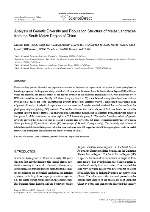
Agricultural Sciences in China2010, 9(9): 1251-1262September 2010Received 30 October, 2009 Accepted 16 April, 2010Analysis of Genetic Diversity and Population Structure of Maize Landraces from the South Maize Region of ChinaLIU Zhi-zhai 1, 2, GUO Rong-hua 2, 3, ZHAO Jiu-ran 4, CAI Yi-lin 1, W ANG Feng-ge 4, CAO Mo-ju 3, W ANG Rong-huan 2, 4, SHI Yun-su 2, SONG Yan-chun 2, WANG Tian-yu 2 and LI Y u 21Maize Research Institute, Southwest University, Chongqing 400716, P.R.China2Institue of Crop Sciences/National Key Facility for Gene Resources and Genetic Improvement, Chinese Academy of Agricultural Sciences,Beijing 100081, P.R.China3Maize Research Institute, Sichuan Agricultural University, Ya’an 625014, P.R.China4Maize Research Center, Beijing Academy of Agricultural and Forestry Sciences, Beijing 100089, P.R.ChinaAbstractUnderstanding genetic diversity and population structure of landraces is important in utilization of these germplasm in breeding programs. In the present study, a total of 143 core maize landraces from the South Maize Region (SR) of China,which can represent the general profile of the genetic diversity in the landraces germplasm of SR, were genotyped by 54DNA microsatellite markers. Totally, 517 alleles (ranging from 4 to 22) were detected among these landraces, with an average of 9.57 alleles per locus. The total gene diversity of these core landraces was 0.61, suggesting a rather higher level of genetic diversity. Analysis of population structure based on Bayesian method obtained the samilar result as the phylogeny neighbor-joining (NJ) method. The results indicated that the whole set of 143 core landraces could be clustered into two distinct groups. All landraces from Guangdong, Hainan, and 15 landraces from Jiangxi were clustered into group 1, while those from the other regions of SR formed the group 2. The results from the analysis of genetic diversity showed that both of groups possessed a similar gene diversity, but group 1 possessed relatively lower mean alleles per locus (6.63) and distinct alleles (91) than group 2 (7.94 and 110, respectively). The relatively high richness of total alleles and distinct alleles preserved in the core landraces from SR suggested that all these germplasm could be useful resources in germplasm enhancement and maize breeding in China.Key words :maize, core landraces, genetic diversity, population structureINTRODUCTIONMaize has been grown in China for nearly 500 years since its first introduction into this second biggest pro-duction country in the world. Currently, there are six different maize growing regions throughout the coun-try according to the ecological conditions and farming systems, including three major production regions,i.e., the North Spring Maize Region, the Huang-Huai-Hai Summer Maize Region, and the Southwest MaizeRegion, and three minor regions, i.e., the South Maize Region, the Northwest Maize Region, and the Qingzang Plateau Maize Region. The South Maize Region (SR)is specific because of its importance in origin of Chi-nese maize. It is hypothesized that Chinese maize is introduced mainly from two routes. One is called the land way in which maize was first brought to Tibet from India, then to Sichuan Province in southwestern China. The other way is that maize dispersed via the oceans, first shipped to the coastal areas of southeast China by boats, and then spread all round the country1252LIU Zhi-zhai et al.(Xu 2001; Zhou 2000). SR contains all of the coastal provinces and regions lie in southeastern China.In the long-term cultivation history of maize in south-ern China, numerous landraces have been formed, in which a great amount of genetic variation was observed (Li 1998). Similar to the hybrid swapping in Europe (Reif et al. 2005a), the maize landraces have been al-most replaced by hybrids since the 1950s in China (Li 1998). However, some landraces with good adapta-tions and yield performances are still grown in a few mountainous areas of this region (Liu et al.1999). Through a great effort of collection since the 1950s, 13521 accessions of maize landraces have been cur-rently preserved in China National Genebank (CNG), and a core collection of these landraces was established (Li et al. 2004). In this core collection, a total of 143 maize landrace accessions were collected from the South Maize Region (SR) (Table 1).Since simple sequence repeat ( SSR ) markers were firstly used in human genetics (Litt and Luty 1989), it now has become one of the most widely used markers in the related researches in crops (Melchinger et al. 1998; Enoki et al. 2005), especially in the molecular characterization of genetic resources, e.g., soybean [Glycine max (L.) Merr] (Xie et al. 2005), rice (Orya sativa L.) (Garris et al. 2005), and wheat (Triticum aestivum) (Chao et al. 2007). In maize (Zea mays L.), numerous studies focusing on the genetic diversity and population structure of landraces and inbred lines in many countries and regions worldwide have been pub-lished (Liu et al. 2003; Vegouroux et al. 2005; Reif et al. 2006; Wang et al. 2008). These activities of documenting genetic diversity and population structure of maize genetic resources have facilitated the under-standing of genetic bases of maize landraces, the utili-zation of these resources, and the mining of favorable alleles from landraces. Although some studies on ge-netic diversity of Chinese maize inbred lines were con-ducted (Yu et al. 2007; Wang et al. 2008), the general profile of genetic diversity in Chinese maize landraces is scarce. Especially, there are not any reports on ge-netic diversity of the maize landraces collected from SR, a possibly earliest maize growing area in China. In this paper, a total of 143 landraces from SR listed in the core collection of CNG were genotyped by using SSR markers, with the aim of revealing genetic diver-sity of the landraces from SR (Table 2) of China and examining genetic relationships and population struc-ture of these landraces.MATERIALS AND METHODSPlant materials and DNA extractionTotally, 143 landraces from SR which are listed in the core collection of CNG established by sequential strati-fication method (Liu et al. 2004) were used in the present study. Detailed information of all these landrace accessions is listed in Table 1. For each landrace, DNA sample was extracted by a CTAB method (Saghi-Maroof et al. 1984) from a bulk pool constructed by an equal-amount of leaves materials sampled from 15 random-chosen plants of each landrace according to the proce-dure of Reif et al. (2005b).SSR genotypingA total of 54 simple sequence repeat (SSR) markers covering the entire maize genome were screened to fin-gerprint all of the 143 core landrace accessions (Table 3). 5´ end of the left primer of each locus was tailed by an M13 sequence of 5´-CACGACGTTGTAAAACGAC-3´. PCR amplification was performed in a 15 L reac-tion containing 80 ng of template DNA, 7.5 mmol L-1 of each of the four dNTPs, 1×Taq polymerase buffer, 1.5 mmol L-1 MgCl2, 1 U Taq polymerase (Tiangen Biotech Co. Ltd., Beijing, China), 1.2 mol L-1 of forward primer and universal fluorescent labeled M13 primer, and 0.3 mol L-1 of M13 sequence tailed reverse primer (Schuelke 2000). The amplification was carried out in a 96-well DNA thermal cycler (GeneAmp PCR System 9700, Applied Biosystem, USA). PCR products were size-separated on an ABI Prism 3730XL DNA sequencer (HitachiHigh-Technologies Corporation, Tokyo, Japan) via the software packages of GENEMAPPER and GeneMarker ver. 6 (SoftGenetics, USA).Data analysesAverage number of alleles per locus and average num-ber of group-specific alleles per locus were identifiedAnalysis of Genetic Diversity and Population Structure of Maize Landraces from the South Maize Region of China 1253Table 1 The detailed information about the landraces used in the present studyPGS revealed by Structure1) NJ dendragram revealed Group 1 Group 2 by phylogenetic analysis140-150tian 00120005AnH-06Jingde Anhui 0.0060.994Group 2170tian00120006AnH-07Jingde Anhui 0.0050.995Group 2Zixihuangyumi00120007AnH-08Zixi Anhui 0.0020.998Group 2Zixibaihuangzayumi 00120008AnH-09Zixi Anhui 0.0030.997Group 2Baiyulu 00120020AnH-10Yuexi Anhui 0.0060.994Group 2Wuhuazi 00120021AnH-11Yuexi Anhui 0.0030.997Group 2Tongbai 00120035AnH-12Tongling Anhui 0.0060.994Group 2Yangyulu 00120036AnH-13Yuexi Anhui 0.0040.996Group 2Huangli 00120037AnH-14Tunxi Anhui 0.0410.959Group 2Baiyumi 00120038AnH-15Tunxi Anhui 0.0030.997Group 2Dapigu00120039AnH-16Tunxi Anhui 0.0350.965Group 2150tianbaiyumi 00120040AnH-17Xiuning Anhui 0.0020.998Group 2Xiuning60tian 00120042AnH-18Xiuning Anhui 0.0040.996Group 2Wubaogu 00120044AnH-19ShitaiAnhui 0.0020.998Group 2Kuyumi00130001FuJ-01Shanghang Fujian 0.0050.995Group 2Zhongdouyumi 00130003FuJ-02Shanghang Fujian 0.0380.962Group 2Baixinyumi 00130004FuJ-03Liancheng Fujian 0.0040.996Group 2Hongxinyumi 00130005FuJ-04Liancheng Fujian 0.0340.966Group 2Baibaogu 00130008FuJ-05Changding Fujian 0.0030.997Group 2Huangyumi 00130011FuJ-06Jiangyang Fujian 0.0020.998Group 2Huabaomi 00130013FuJ-07Shaowu Fujian 0.0020.998Group 2Huangbaomi 00130014FuJ-08Songxi Fujian 0.0020.998Group 2Huangyumi 00130016FuJ-09Wuyishan Fujian 0.0460.954Group 2Huabaogu 00130019FuJ-10Jian’ou Fujian 0.0060.994Group 2Huangyumi 00130024FuJ-11Guangze Fujian 0.0010.999Group 2Huayumi 00130025FuJ-12Nanping Fujian 0.0040.996Group 2Huangyumi 00130026FuJ-13Nanping Fujian 0.0110.989Group 2Hongbaosu 00130027FuJ-14Longyan Fujian 0.0160.984Group 2Huangfansu 00130029FuJ-15Loangyan Fujian 0.0020.998Group 2Huangbaosu 00130031FuJ-16Zhangping Fujian 0.0060.994Group 2Huangfansu 00130033FuJ-17Zhangping Fujian0.0040.996Group 2Baolieyumi 00190001GuangD-01Guangzhou Guangdong 0.9890.011Group 1Nuomibao (I)00190005GuangD-02Shixing Guangdong 0.9740.026Group 1Nuomibao (II)00190006GuangD-03Shixing Guangdong 0.9790.021Group 1Zasehuabao 00190010GuangD-04Lechang Guangdong 0.9970.003Group 1Zihongmi 00190013GuangD-05Lechang Guangdong 0.9880.012Group 1Jiufengyumi 00190015GuangD-06Lechang Guangdong 0.9950.005Group 1Huangbaosu 00190029GuangD-07MeiGuangdong 0.9970.003Group 1Bailibao 00190032GuangD-08Xingning Guangdong 0.9980.002Group 1Nuobao00190038GuangD-09Xingning Guangdong 0.9980.002Group 1Jinlanghuang 00190048GuangD-10Jiangcheng Guangdong 0.9960.004Group 1Baimizhenzhusu 00190050GuangD-11Yangdong Guangdong 0.9940.006Group 1Huangmizhenzhusu 00190052GuangD-12Yangdong Guangdong 0.9930.007Group 1Baizhenzhu 00190061GuangD-13Yangdong Guangdong 0.9970.003Group 1Baiyumi 00190066GuangD-14Wuchuan Guangdong 0.9880.012Group 1Bendibai 00190067GuangD-15Suixi Guangdong 0.9980.002Group 1Shigubaisu 00190068GuangD-16Gaozhou Guangdong 0.9960.004Group 1Zhenzhusu 00190069GuangD-17Xinyi Guangdong 0.9960.004Group 1Nianyaxixinbai 00190070GuangD-18Huazhou Guangdong 0.9960.004Group 1Huangbaosu 00190074GuangD-19Xinxing Guangdong 0.9950.005Group 1Huangmisu 00190076GuangD-20Luoding Guangdong 0.940.060Group 1Huangmi’ai 00190078GuangD-21Luoding Guangdong 0.9980.002Group 1Bayuemai 00190084GuangD-22Liannan Guangdong 0.9910.009Group 1Baiyumi 00300001HaiN-01Haikou Hainan 0.9960.004Group 1Baiyumi 00300003HaiN-02Sanya Hainan 0.9970.003Group 1Hongyumi 00300004HaiN-03Sanya Hainan 0.9980.002Group 1Baiyumi00300011HaiN-04Tongshi Hainan 0.9990.001Group 1Zhenzhuyumi 00300013HaiN-05Tongshi Hainan 0.9980.002Group 1Zhenzhuyumi 00300015HaiN-06Qiongshan Hainan 0.9960.004Group 1Aiyumi 00300016HaiN-07Qiongshan Hainan 0.9960.004Group 1Huangyumi 00300021HaiN-08Qionghai Hainan 0.9970.003Group 1Y umi 00300025HaiN-09Qionghai Hainan 0.9870.013Group 1Accession name Entry code Analyzing code Origin (county/city)Province/Region1254LIU Zhi-zhai et al .Baiyumi00300032HaiN-10Tunchang Hainan 0.9960.004Group 1Huangyumi 00300051HaiN-11Baisha Hainan 0.9980.002Group 1Baihuangyumi 00300055HaiN-12BaishaHainan 0.9970.003Group 1Machihuangyumi 00300069HaiN-13Changjiang Hainan 0.9900.010Group 1Hongyumi00300073HaiN-14Dongfang Hainan 0.9980.002Group 1Xiaohonghuayumi 00300087HaiN-15Lingshui Hainan 0.9980.002Group 1Baiyumi00300095HaiN-16Qiongzhong Hainan 0.9950.005Group 1Y umi (Baimai)00300101HaiN-17Qiongzhong Hainan 0.9980.002Group 1Y umi (Xuemai)00300103HaiN-18Qiongzhong Hainan 0.9990.001Group 1Huangmaya 00100008JiangS-10Rugao Jiangsu 0.0040.996Group 2Bainian00100012JiangS-11Rugao Jiangsu 0.0080.992Group 2Bayebaiyumi 00100016JiangS-12Rudong Jiangsu 0.0040.996Group 2Chengtuohuang 00100021JiangS-13Qidong Jiangsu 0.0050.995Group 2Xuehuanuo 00100024JiangS-14Qidong Jiangsu 0.0020.998Group 2Laobaiyumi 00100032JiangS-15Qidong Jiangsu 0.0050.995Group 2Laobaiyumi 00100033JiangS-16Qidong Jiangsu 0.0010.999Group 2Huangwuye’er 00100035JiangS-17Hai’an Jiangsu 0.0030.997Group 2Xiangchuanhuang 00100047JiangS-18Nantong Jiangsu 0.0060.994Group 2Huangyingzi 00100094JiangS-19Xinghua Jiangsu 0.0040.996Group 2Xiaojinhuang 00100096JiangS-20Yangzhou Jiangsu 0.0010.999Group 2Liushizi00100106JiangS-21Dongtai Jiangsu 0.0030.997Group 2Kangnandabaizi 00100108JiangS-22Dongtai Jiangsu 0.0020.998Group 2Shanyumi 00140020JiangX-01Dexing Jiangxi 0.9970.003Group 1Y umi00140024JiangX-02Dexing Jiangxi 0.9970.003Group 1Tianhongyumi 00140027JiangX-03Yushan Jiangxi 0.9910.009Group 1Hongganshanyumi 00140028JiangX-04Yushan Jiangxi 0.9980.002Group 1Zaoshuyumi 00140032JiangX-05Qianshan Jiangxi 0.9970.003Group 1Y umi 00140034JiangX-06Wannian Jiangxi 0.9970.003Group 1Y umi 00140038JiangX-07De’an Jiangxi 0.9940.006Group 1Y umi00140045JiangX-08Wuning Jiangxi 0.9740.026Group 1Chihongyumi 00140049JiangX-09Wanzai Jiangxi 0.9920.008Group 1Y umi 00140052JiangX-10Wanzai Jiangxi 0.9930.007Group 1Huayumi 00140060JiangX-11Jing’an Jiangxi 0.9970.003Group 1Baiyumi 00140065JiangX-12Pingxiang Jiangxi 0.9940.006Group 1Huangyumi00140066JiangX-13Pingxiang Jiangxi 0.9680.032Group 1Nuobaosuhuang 00140068JiangX-14Ruijin Jiangxi 0.9950.005Group 1Huangyumi 00140072JiangX-15Xinfeng Jiangxi 0.9960.004Group 1Wuningyumi 00140002JiangX-16Jiujiang Jiangxi 0.0590.941Group 2Tianyumi 00140005JiangX-17Shangrao Jiangxi 0.0020.998Group 2Y umi 00140006JiangX-18Shangrao Jiangxi 0.0310.969Group 2Baiyiumi 00140012JiangX-19Maoyuan Jiangxi 0.0060.994Group 260riyumi 00140016JiangX-20Maoyuan Jiangxi 0.0020.998Group 2Shanyumi 00140019JiangX-21Dexing Jiangxi 0.0050.995Group 2Laorenya 00090002ShangH-01Chongming Shanghai 0.0050.995Group 2Jinmeihuang 00090004ShangH-02Chongming Shanghai 0.0020.998Group 2Zaobaiyumi 00090006ShangH-03Chongming Shanghai 0.0020.998Group 2Chengtuohuang 00090007ShangH-04Chongming Shanghai 0.0780.922Group 2Benyumi (Huang)00090008ShangH-05Shangshi Shanghai 0.0020.998Group 2Bendiyumi 00090010ShangH-06Shangshi Shanghai 0.0040.996Group 2Baigengyumi 00090011ShangH-07Jiading Shanghai 0.0020.998Group 2Huangnuoyumi 00090012ShangH-08Jiading Shanghai 0.0040.996Group 2Huangdubaiyumi 00090013ShangH-09Jiading Shanghai 0.0440.956Group 2Bainuoyumi 00090014ShangH-10Chuansha Shanghai 0.0010.999Group 2Laorenya 00090015ShangH-11Shangshi Shanghai 0.0100.990Group 2Xiaojinhuang 00090016ShangH-12Shangshi Shanghai 0.0050.995Group 2Gengbaidayumi 00090017ShangH-13Shangshi Shanghai 0.0020.998Group 2Nongmeiyihao 00090018ShangH-14Shangshi Shanghai 0.0540.946Group 2Chuanshazinuo 00090020ShangH-15Chuansha Shanghai 0.0550.945Group 2Baoanshanyumi 00110004ZheJ-01Jiangshan Zhejiang 0.0130.987Group 2Changtaixizi 00110005ZheJ-02Jiangshan Zhejiang 0.0020.998Group 2Shanyumibaizi 00110007ZheJ-03Jiangshan Zhejiang 0.0020.998Group 2Kaihuajinyinbao 00110017ZheJ-04Kaihua Zhejiang 0.0100.990Group 2Table 1 (Continued from the preceding page)PGS revealed by Structure 1) NJ dendragram revealed Group1 Group2 by phylogenetic analysisAccession name Entry code Analyzing code Origin (county/city)Province/RegoinAnalysis of Genetic Diversity and Population Structure of Maize Landraces from the South Maize Region of China 1255Liputianzi00110038ZheJ-05Jinhua Zhejiang 0.0020.998Group 2Jinhuaqiuyumi 00110040ZheJ-06Jinhua Zhejiang 0.0050.995Group 2Pujiang80ri 00110069ZheJ-07Pujiang Zhejiang 0.0210.979Group 2Dalihuang 00110076ZheJ-08Yongkang Zhejiang 0.0140.986Group 2Ziyumi00110077ZheJ-09Yongkang Zhejiang 0.0020.998Group 2Baiyanhandipinzhong 00110078ZheJ-10Yongkang Zhejiang 0.0030.997Group 2Duosuiyumi00110081ZheJ-11Wuyi Zhejiang 0.0020.998Group 2Chun’an80huang 00110084ZheJ-12Chun’an Zhejiang 0.0020.998Group 2120ribaiyumi 00110090ZheJ-13Chun’an Zhejiang 0.0020.998Group 2Lin’anliugu 00110111ZheJ-14Lin’an Zhejiang 0.0030.997Group 2Qianhuangyumi00110114ZheJ-15Lin’an Zhejiang 0.0030.997Group 2Fenshuishuitianyumi 00110118ZheJ-16Tonglu Zhejiang 0.0410.959Group 2Kuihualiugu 00110119ZheJ-17Tonglu Zhejiang 0.0030.997Group 2Danbaihuang 00110122ZheJ-18Tonglu Zhejiang 0.0020.998Group 2Hongxinma 00110124ZheJ-19Jiande Zhejiang 0.0030.997Group 2Shanyumi 00110136ZheJ-20Suichang Zhejiang 0.0030.997Group 2Bai60ri 00110143ZheJ-21Lishui Zhejiang 0.0050.995Group 2Zeibutou 00110195ZheJ-22Xianju Zhejiang 0.0020.998Group 2Kelilao00110197ZheJ-23Pan’an Zhejiang 0.0600.940Group 21)The figures refered to the proportion of membership that each landrace possessed.Table 1 (Continued from the preceding page)PGS revealed by Structure 1) NJ dendragram revealed Group 1 Group 2 by phylogenetic analysisAccession name Entry code Analyzing code Origin (county/city)Province/Regoin Table 2 Construction of two phylogenetic groups (SSR-clustered groups) and their correlation with geographical locationsGeographical location SSR-clustered groupChi-square testGroup 1Group 2Total Guangdong 2222 χ2 = 124.89Hainan 1818P < 0.0001Jiangxi 15621Anhui 1414Fujian 1717Jiangsu 1313Shanghai 1515Zhejiang 2323Total5588143by the software of Excel MicroSatellite toolkit (Park 2001). Average number of alleles per locus was calcu-lated by the formula rAA rj j¦1, with the standarddeviation of1)()(12¦ r A AA rj jV , where A j was thenumber of distinct alleles at locus j , and r was the num-ber of loci (Park 2001).Unbiased gene diversity also known as expected heterozygosity, observed heterozygosity for each lo-cus and average gene diversity across the 54 SSR loci,as well as model-based groupings inferred by Struc-ture ver. 2.2, were calculated by the softwarePowerMarker ver.3.25 (Liu et al . 2005). Unbiased gene diversity for each locus was calculated by˅˄¦ 2ˆ1122ˆi x n n h , where 2ˆˆ2ˆ2¦¦z ji ijij i X X x ,and ij X ˆwas the frequency of genotype A i A jin the sample, and n was the number of individuals sampled.The average gene diversity across 54 loci was cal-culated as described by Nei (1987) as follows:rh H rj j ¦1ˆ, with the variance ,whereThe average observed heterozygosity across the en-tire loci was calculated as described by (Hedrick 1983)as follows: r jrj obsobs n h h ¦1, with the standard deviationrn h obs obsobs 1V1256LIU Zhi-zhai et al.Phylogenetic analysis and population genetic structureRelationships among all of the 143 accessions collected from SR were evaluated by using the unweighted pair group method with neighbor-joining (NJ) based on the log transformation of the proportion of shared alleles distance (InSPAD) via PowerMarker ver. 3.25 (FukunagaTable 3 The PIC of each locus and the number of alleles detected by 54 SSRsLocus Bin Repeat motif PIC No. of alleles Description 2)bnlg1007y51) 1.02AG0.7815Probe siteumc1122 1.06GGT0.639Probe siteumc1147y41) 1.07CA0.2615Probe sitephi961001) 2.00ACCT0.298Probe siteumc1185 2.03GC0.7215ole1 (oleosin 1)phi127 2.08AGAC0.577Probe siteumc1736y21) 2.09GCA T0.677Probe sitephi453121 3.01ACC0.7111Probe sitephi374118 3.03ACC0.477Probe sitephi053k21) 3.05A TAC0.7910Probe sitenc004 4.03AG0.4812adh2 (alcohol dehydrogenase 2)bnlg490y41) 4.04T A0.5217Probe sitephi079 4.05AGATG0.495gpc1(glyceraldehyde-3-phosphate dehydrogenase 1) bnlg1784 4.07AG0.6210Probe siteumc1574 4.09GCC0.719sbp2 (SBP-domain protein 2)umc1940y51) 4.09GCA0.4713Probe siteumc1050 4.11AA T0.7810cat3 (catalase 3)nc130 5.00AGC0.5610Probe siteumc2112y31) 5.02GA0.7014Probe sitephi109188 5.03AAAG0.719Probe siteumc1860 5.04A T0.325Probe sitephi085 5.07AACGC0.537gln4 (glutamine synthetase 4)phi331888 5.07AAG0.5811Probe siteumc1153 5.09TCA0.7310Probe sitephi075 6.00CT0.758fdx1 (ferredoxin 1)bnlg249k21) 6.01AG0.7314Probe sitephi389203 6.03AGC0.416Probe sitephi299852y21) 6.07AGC0.7112Probe siteumc1545y21)7.00AAGA0.7610hsp3(heat shock protein 3)phi1127.01AG0.5310o2 (opaque endosperm 2)phi4207018.00CCG0.469Probe siteumc13598.00TC0.7814Probe siteumc11398.01GAC0.479Probe siteumc13048.02TCGA0.335Probe sitephi1158.03A TAC0.465act1(actin1)umc22128.05ACG0.455Probe siteumc11218.05AGAT0.484Probe sitephi0808.08AGGAG0.646gst1 (glutathione-S-transferase 1)phi233376y11)8.09CCG0.598Probe sitebnlg12729.00AG0.8922Probe siteumc20849.01CTAG0.498Probe sitebnlg1520k11)9.01AG0.5913Probe sitephi0659.03CACCT0.519pep1(phosphoenolpyruvate carboxylase 1)umc1492y131)9.04GCT0.2514Probe siteumc1231k41)9.05GA0.2210Probe sitephi1084119.06AGCT0.495Probe sitephi4488809.06AAG0.7610Probe siteumc16759.07CGCC0.677Probe sitephi041y61)10.00AGCC0.417Probe siteumc1432y61)10.02AG0.7512Probe siteumc136710.03CGA0.6410Probe siteumc201610.03ACAT0.517pao1 (polyamine oxidase 1)phi06210.04ACG0.337mgs1 (male-gametophyte specific 1)phi07110.04GGA0.515hsp90 (heat shock protein, 90 kDa)1) These primers were provided by Beijing Academy of Agricultural and Forestry Sciences (Beijing, China).2) Searched from Analysis of Genetic Diversity and Population Structure of Maize Landraces from the South Maize Region of China1257et al. 2005). The unrooted phylogenetic tree was finally schematized with the software MEGA (molecular evolu-tionary genetics analysis) ver. 3.1 (Kumar et al. 2004). Additionally, a chi-square test was used to reveal the correlation between the geographical origins and SSR-clustered groups through FREQ procedure implemented in SAS ver. 9.0 (2002, SAS Institute, Inc.).In order to reveal the population genetic structure (PGS) of 143 landrace accessions, a Bayesian approach was firstly applied to determine the number of groups (K) that these materials should be assigned by the soft-ware BAPS (Bayesian Analysis of Population Structure) ver.5.1. By using BAPS, a fixed-K clustering proce-dure was applied, and with each separate K, the num-ber of runs was set to 100, and the value of log (mL) was averaged to determine the appropriate K value (Corander et al. 2003; Corander and Tang 2007). Since the number of groups were determined, a model-based clustering analysis was used to assign all of the acces-sions into the corresponding groups by an admixture model and a correlated allele frequency via software Structure ver.2.2 (Pritchard et al. 2000; Falush et al. 2007), and for the given K value determined by BAPS, three independent runs were carried out by setting both the burn-in period and replication number 100000. The threshold probability assigned individuals into groupswas set by 0.8 (Liu et al. 2003). The PGS result carried out by Structure was visualized via Distruct program ver. 1.1 (Rosenberg 2004).RESULTSGenetic diversityA total of 517 alleles were detected by the whole set of54 SSRs covering the entire maize genome through all of the 143 maize landraces, with an average of 9.57 alleles per locus and ranged from 4 (umc1121) to 22 (bnlg1272) (Table 3). Among all the alleles detected, the number of distinct alleles accounted for 132 (25.53%), with an av-erage of 2.44 alleles per locus. The distinct alleles dif-fered significantly among the landraces from different provinces/regions, and the landraces from Guangdong, Fujian, Zhejiang, and Shanghai possessed more distinct alleles than those from the other provinces/regions, while those from southern Anhui possessed the lowest distinct alleles, only counting for 3.28% of the total (Table 4).Table 4 The genetic diversity within eight provinces/regions and groups revealed by 54 SSRsProvince/Region Sample size Allele no.1)Distinct allele no.Gene diversity (expected heterozygosity)Observed heterozygosity Anhui14 4.28 (4.19) 69 (72.4)0.51 (0.54)0.58 (0.58)Fujian17 4.93 (4.58 80 (79.3)0.56 (0.60)0.63 (0.62)Guangdong22 5.48 (4.67) 88 (80.4)0.57 (0.59)0.59 (0.58)Hainan18 4.65 (4.26) 79 (75.9)0.53 (0.57)0.55 (0.59)Jiangsu13 4.24 700.500.55Jiangxi21 4.96 (4.35) 72 (68.7)0.56 (0.60)0.68 (0.68)Shanghai15 5.07 (4.89) 90 (91.4)0.55 (0.60)0.55 (0.55)Zhejiang23 5.04 (4.24) 85 (74)0.53 (0.550.60 (0.61)Total/average1439.571320.610.60GroupGroup 155 6.63 (6.40) 91 (89.5)0.57 (0.58)0.62 (0.62)Group 2887.94 (6.72)110 (104.3)0.57 (0.57)0.59 (0.58)Total/Average1439.571320.610.60Provinces/Regions within a groupGroup 1Total55 6.69 (6.40) 910.57 (0.58)0.62 (0.62)Guangdong22 5.48 (4.99) 86 (90.1)0.57 (0.60)0.59 (0.58)Hainan18 4.65 (4.38) 79 (73.9)0.53 (0.56)0.55 (0.59)Jiangxi15 4.30 680.540.69Group 2Total887.97 (6.72)110 (104.3)0.57 (0.57)0.59 (0.58)Anhui14 4.28 (3.22) 69 (63.2)0.51 (0.54)0.58 (0.57)Fujian17 4.93 (3.58) 78 (76.6)0.56 (0.60)0.63 (0.61)Jiangsu13 4.24 (3.22) 71 (64.3)0.50 (0.54)0.55 (0.54)Jiangxi6 3.07 520.460.65Shanghai15 5.07 (3.20) 91 (84.1)0.55 (0.60)0.55 (0.54)Zhejiang23 5.04 (3.20) 83 (61.7)0.53 (0.54)0.60 (0.58)1258LIU Zhi-zhai et al.Among the 54 loci used in the study, 16 (or 29.63%) were dinucleotide repeat SSRs, which were defined as type class I-I, the other 38 loci were SSRs with a longer repeat motifs, and two with unknown repeat motifs, all these 38 loci were defined as the class of I-II. In addition, 15 were located within certain functional genes (defined as class II-I) and the rest were defined as class II-II. The results of comparison indicated that the av-erage number of alleles per locus captured by class I-I and II-II were 12.88 and 10.05, respectively, which were significantly higher than that by type I-II and II-I (8.18 and 8.38, respectively). The gene diversity re-vealed by class I-I (0.63) and II-I (0.63) were some-what higher than by class I-II (0.60) and II-II (0.60) (Table 5).Genetic relationships of the core landraces Overall, 143 landraces were clustered into two groups by using neighbor-joining (NJ) method based on InSPAD. All the landraces from provinces of Guangdong and Hainan and 15 of 21 from Jiangxi were clustered together to form group 1, and the other 88 landraces from the other provinces/regions formed group 2 (Fig.-B). The geographical origins of all these 143 landraces with the clustering results were schematized in Fig.-D. Revealed by the chi-square test, the phylogenetic results (SSR-clustered groups) of all the 143 landraces from provinces/regions showed a significant correlation with their geographical origin (χ2=124.89, P<0.0001, Table 2).Revealed by the phylogenetic analysis based on the InSPAD, the minimum distance was observed as 0.1671 between two landraces, i.e., Tianhongyumi (JiangX-03) and Hongganshanyumi (JiangX-04) collected from Jiangxi Province, and the maximum was between two landraces of Huangbaosu (FuJ-16) and Hongyumi (HaiN-14) collected from provinces of Fujian and Hainan, respectively, with the distance of 1.3863 (data not shown). Two landraces (JiangX-01 and JiangX-21) collected from the same location of Dexing County (Table 1) possessing the same names as Shanyumi were separated to different groups, i.e., JiangX-01 to group1, while JiangX-21 to group 2 (Table 1). Besides, JiangX-01 and JiangX-21 showed a rather distant distance of 0.9808 (data not shown). These results indicated that JiangX-01 and JiangX-21 possibly had different ances-tral origins.Population structureA Bayesian method was used to detect the number of groups (K value) of the whole set of landraces from SR with a fixed-K clustering procedure implemented in BAPS software ver. 5.1. The result showed that all of the 143 landraces could also be assigned into two groups (Fig.-A). Then, a model-based clustering method was applied to carry out the PGS of all the landraces via Structure ver. 2.2 by setting K=2. This method as-signed individuals to groups based on the membership probability, thus the threshold probability 0.80 was set for the individuals’ assignment (Liu et al. 2003). Accordingly, all of the 143 landraces were divided into two distinct model-based groups (Fig.-C). The landraces from Guangdong, Hainan, and 15 landraces from Jiangxi formed one group, while the rest 6 landraces from the marginal countries of northern Jiangxi and those from the other provinces formed an-other group (Table 1, Fig.-D). The PGS revealed by the model-based approach via Structure was perfectly consistent with the relationships resulted from the phy-logenetic analysis via PowerMarker (Table 1).DISCUSSIONThe SR includes eight provinces, i.e., southern Jiangsu and Anhui, Shanghai, Zhejiang, Fujian, Jiangxi, Guangdong, and Hainan (Fig.-C), with the annual maize growing area of about 1 million ha (less than 5% of theTable 5 The genetic diversity detected with different types of SSR markersType of locus No. of alleles Gene diversity Expected heterozygosity PIC Class I-I12.880.630.650.60 Class I-II8.180.600.580.55 Class II-I8.330.630.630.58。
基于自适应遗传算法的多无人机协同任务分配
2021,36(1)电子信息对抗技术Electronic Information Warfare Technology㊀㊀中图分类号:V279;TN97㊀㊀㊀㊀㊀㊀文献标志码:A㊀㊀㊀㊀㊀㊀文章编号:1674-2230(2021)01-0059-06收稿日期:2020-02-28;修回日期:2020-03-30作者简介:王树朋(1990 ),男,博士,工程师㊂基于自适应遗传算法的多无人机协同任务分配王树朋,徐㊀旺,刘湘德,邓小龙(电子信息控制重点实验室,成都610036)摘要:提出一种自适应遗传算法,利用基于任务价值㊁飞行航程和任务分配均衡性的适应度函数评估任务分配方案的优劣,在算法运行过程中交叉率和变异率进行实时动态调整,以克服标准遗传算法易陷入局部最优的缺点㊂将提出的自适应遗传算法用于多无人机协同任务分配问题的求解,设置并进行了实验㊂实验结果表明:提出的自适应遗传算法可以较好地解决多无人机协同任务分配问题,得到较高的作战效能,证明了该方法的有效性㊂关键词:遗传算法;适应度函数;无人机;任务分配;作战效能DOI :10.3969/j.issn.1674-2230.2021.01.013Cooperative Task Assignment for Multi -UAVBased on Adaptive Genetic AlgorithmWANG Shupeng,XU Wang,LIU Xiangde,DENG Xiaolong(Science and Technology on Electronic Information Control Laboratory,Chengdu 610036,China)Abstract :An improved adaptive genetic algorithm is proposed,and a fitness function based ontask value,flying distance and the balance of task allocation scheme is used to evaluate the qualityof task allocation schemes.In the proposed algorithm,the crossover probability and mutation prob-ability can adjust automatically to avoid effectively the phenomenon of the standard genetic algo-rithm falling into the local optimum.The proposed improved genetic algorithm is used to solve the problem of cooperative task assignment for multiple Unmanned Aerial Vehicles (UAVs).The ex-periments are conducted and the experimental results show that the proposed adaptive genetic al-gorithm can significantly solve the problem and obtain an excellent combat effectiveness.The ef-fectiveness of the proposed method is demonstrated with the experimental results.Key words :genetic algorithm;fitness function;UAV;task assignment;combat effectiveness1㊀引言无人机是一种依靠程序自主操纵或受无线遥控的飞行器[1],在军事科技方面得到了极大重视,是新颖军事技术和新型武器平台的杰出代表㊂随着战场环境日益复杂,对于无人机的性能要求越来越高,单一无人机在复杂的战场环境中执行任务具有诸多不足,通常多个无人机进行协同作战或者执行任务㊂通常地,多无人机协同任务分配是:在无人机种类和数量已知的情况下,基于一定的环境信息和任务需求,为多个无人机分配一个或者一组有序的任务,要求在完成任务最大化的同时,多个无人机任务执行的整体效能最大,且所付出的代价最小㊂从理论上讲,多无人机协同任务分配属于NP -hard 的组合优化问题,通常需95王树朋,徐㊀旺,刘湘德,邓小龙基于自适应遗传算法的多无人机协同任务分配投稿邮箱:dzxxdkjs@要借助于算法进行求解㊂目前,国内外研究人员已经对于多无人机协同任务分配问题进行了大量的研究,并提出很多用于解决该问题的算法,主要有:群算法㊁自由市场机制算法和进化算法等㊂群算法是模拟自然界生物群体的行为的算法,其中蚁群算法[2-3]㊁粒子群算法[4]以及鱼群算法[5]是最为典型的群算法㊂研究人员发现群算法可以用于求解多无人机协同任务分配问题,但是该算法极易得到局部最优而非全局最优㊂自由市场机制算法[6]是利用明确的规则引导买卖双方进行公开竞价,在短时间内将资源合理化,得到问题的最优解和较优解㊂进化算法适合求解大规模问题,其中遗传算法[7-8]是最著名的进化算法㊂遗传算法在运行过程中会出现不容易收敛或陷入局部最优的问题,许多研究人员针对该问题对遗传算法进行了改进㊂本文提出一种改进的自适应遗传算法,在算法运行过程中适应度值㊁交叉率和变异率可以进行实时动态调整,以克服遗传算法易陷入局部最优的缺点,并利用该算法解决多无人机协同任务分配问题,以求在满足一定的约束条件下,无人机执行任务的整体收益最大,同时付出的代价最小,得到较大的效费比㊂2㊀问题描述㊀㊀多无人机协同任务分配模型是通过设置并满足一定约束条件的情况下,包括无人机的自身能力限制和环境以及任务的要求等,估算各个无人机执行任务获得的收益以及付出的代价,并利用评价指标进行评价,以求得到最大的收益损耗比和最优作战效能㊂通常情况下,多无人机协同任务分配需满足以下约束:1)每个任务只能被分配一次;2)无人机可以携带燃料限制造成的最大航程约束;3)无人机载荷限制,无人机要执行某项任务必须装载相应的载荷㊂另外,多无人机协同任务分配需要遵循以下原则:1)收益最高:每项任务都拥有它的价值,任务分配方案应该得到最大整体收益;2)航程最小:应该尽快完成任务,尽可能减小飞行航程,这样易满足无人机的航程限制,同时降低无人机面临的威胁;3)各个无人机的任务负载尽可能均衡,通常以任务个数或者飞行航程作为标准判定; 4)优先执行价值高的任务㊂根据以上原则,提出多无人机协同任务分配的评价指标,包括:1)任务价值指标:用于评估任务分配方案可以得到的整体收益;2)任务分配均衡性指标:用于评估无人机的任务负载是否均衡;3)飞行航程指标:用于评估无人机的飞行航程㊂3㊀遗传算法㊀㊀要将遗传算法用于多无人机协同任务分配问题的求解,可以将任务分配方案当作种群中的个体,确定合适的染色体编码方法,利用按照一定结构组成的染色体表示任务分配方案㊂然后,通过选择㊁交叉和变异等遗传操作进行不断进化,直到满足约束条件㊂通常来说,遗传算法可以表示为GA=(C,E, P0,M,F,G,Y,T),其中C㊁E㊁P0和M分别表示染色体编码方法㊁适应度函数㊁初始种群和种群大小,在本文的应用中,P0和M分别表示初始的任务分配方案集合以及任务分配方案的个数;F㊁G 和Y分别表示选择算子㊁交叉算子和变异算子;T 表示终止的条件和规则㊂因此,利用遗传算法解决多无人机协同任务分配问题的主要工作是确定以上8个参数㊂3.1㊀编码方法利用由一定结构组成的染色体表示任务分配方案,将一个任务分配方案转换为一条染色体的过程可以分为2个步骤:第一步是根据各个无人机需执行的任务确定各个无人机对应的染色体;第二步是将这些小的染色体结合,形成整个任务分配方案对应的完整染色体㊂假设无人机和任务的个数分别为N u和N t,其中第i个无人机U i的06电子信息对抗技术㊃第36卷2021年1月第1期王树朋,徐㊀旺,刘湘德,邓小龙基于自适应遗传算法的多无人机协同任务分配任务共有k个,分别是T i1㊁T i2㊁ ㊁T ik,则该无人机对应的任务染色体为[T i1T i2 T ik]㊂在任务分配时,可能出现N t个任务全部分配给一个无人机的情况,另外为增加随机性和扩展性,提高遗传算法的全局搜索能力,随机将N t-k个0插入到以上的任务染色体中,产生一条全新的长度为N t的染色体㊂最终,一个任务分配方案可以转换为一条长度为N u∗N t的染色体㊂3.2㊀适应度函数在本文的应用中,适应度函数E是用于判断任务分配方案的质量,根据上文提出的多无人机协同任务分配问题的原则和评价指标可知,主要利用任务价值指标㊁任务分配均衡性指标以及飞行航程指标等三个指标判定任务分配方案的质量㊂假设有N u个无人机,F i表示第i个无人机U i的飞行航程,整个任务的总飞行航程F t可以表示为:F t=ðN u i=1F i(1)无人机的平均航程为:F=F t Nu(2)无人机飞行航程的方差D可以表示为:D=ðN u i=1F i-F-()2N u(3)为充分考虑任务价值㊁飞行航程以及各个无人机任务的均衡性,将任务分配方案的适应度函数定义为:E=V ta∗F t+b∗D(4)其中:V t为任务的总价值,F t为总飞行航程,D为各个无人机飞行航程的方差,a和b分别表示飞行航程以及飞行航程均衡性的权重㊂另外,任务分配方案的收益损耗比GL可以表示为:GL=V tF t(5)另外,在遗传算法运行的不同阶段,需要对任务分配方案的适应度进行适当地扩大或者缩小,新的适应度函数E可以表示为:Eᶄ=1-e-αEα=m tE max-E avg+1,m=1+lg T()ìîíïïïï(6)其中:E为利用公式(4)计算得到的原适应度值, E avg为适应度值的平均值,E max为适应度最大值,t 为算法的运行次数,T为遗传算法的终止条件㊂在遗传算法运行初期,E max-E avg较大,而t较小,因此α较小,可以提高低质量任务分配方案的选择概率,同时降低高质量任务分配方案的选择概率;随着算法的运行,E max-E avg将逐渐减小,t 将逐渐增大,因此α会逐渐增大,可以避免算法陷入随机选择和局部最优㊂3.3㊀种群大小㊁初始种群和终止条件按照通常做法,将种群大小M的取值范围设定为20~100㊂首先,随机产生2∗M个符合要求的任务分配方案,利用公式(4)计算各个任务分配方案的适应度值㊂然后,从中选取出适应度值较高的M 个任务分配方案组成初始种群P0,即初始任务分配方案集合㊂终止条件T设定为:在规定的迭代次数内有一个任务分配方案的适应度值满足条件,则停止进化;否则,一直运行到规定的迭代次数㊂3.4㊀选择算子首先,采用精英保留策略将当前适应度值最大的一个任务分配方案直接保留到下一代,提高遗传算法的全局收敛能力㊂随后,利用最知名的轮盘赌选择法选择出剩余的任务分配方案㊂3.5㊀交叉算子和变异算子在算法运行过程中需随时动态调整p c和p m,动态调整的原则如下:1)适当降低适应度值比平均适应度值高的任务分配方案的p c和p m,以保护优秀的高质量任务分配方案,加快算法的收敛速度;2)适当增大适应度值比平均适应度值低的任务分配方案的p c和p m,以免算法陷入局部最优㊂另外,任务分配方案的集中度β也是决定p c 和p m的重要因素,β可以表示为:16王树朋,徐㊀旺,刘湘德,邓小龙基于自适应遗传算法的多无人机协同任务分配投稿邮箱:dzxxdkjs@β=E avgE max(7)其中:E avg 表示平均适应度值;E max 表示最大适应度值㊂显然,β越大,任务分配方案越集中,遗传算法越容易陷入局部最优㊂因此,随着β增大,p c 和p m 应该随之增大㊂基于以上原则,定义p c 和p m 如下:p c =0.8E avg -Eᵡ()+0.6Eᵡ-E min ()E avg -E min +0.2㊃βEᵡ<E avg 0.6E max -Eᵡ()+0.4Eᵡ-E avg ()E max -E avg +0.2㊃βEᵡȡE avgìîíïïïïïp m =0.08E avg -E‴()+0.05E‴-E min ()E avg -E min +0.02㊃βE‴<E avg and β<0.80.05E max -E‴()+0.0001E‴-E avg ()E max -E avg+0.02㊃βE‴ȡE avg and β<0.80.5βȡ0.8ìîíïïïïïï(8)其中:E max 为最大适应度值,E min 为最小适应度值,E avg 为平均适应度值,Eᵡ为进行交叉操作的两个任务分配方案中的较大适应度值,E‴为进行变异操作的任务分配方案的适应度值,β为任务分配方案的集中度,可利用公式(7)计算得到㊂4㊀实验结果4.1㊀实验设置4架无人机从指定的起飞机场起飞,飞至5个任务目标点执行10项任务,最终降落到指定的降落机场㊂其中,如表1所示,无人机的编号分别为UAV 1㊁UAV 2㊁UAV 3和UAV 4㊂另外,起飞机场㊁降落机场㊁目标如图6所示㊂任务的编号分别为任务1至任务10(简称为T 1㊁T 2㊁ ㊁T 10),每项任务均为到某一个目标点执行侦察㊁攻击㊁事后评估中的某一项,任务设置如表2所示㊂表1㊀无人机信息编号最大航程装载载荷UAV 120侦察㊁攻击UAV 120侦察UAV 125攻击㊁评估UAV 130侦察㊁评估图1㊀任务目标位置示意图表2㊀任务设置任务编号目标编号任务类型任务价值T 11侦察1T 21攻击2T 32攻击3T 42评估3T 53侦察4T 63评估6T 74侦察2T 84攻击3T 94评估5T 105评估14.2㊀第一组实验首先,随机地进行任务分配,得到一个满足多无人机协同任务分配的约束条件的任务分配方案如下:㊃UAV 1:T 2ңT 5㊃UAV 2:T 1ңT 7㊃UAV 3:T 3ңT 6ңT 8㊃UAV 4:T 4ңT 9ңT 10计算可知,4个无人机的飞行航程分别是14.0674㊁12.6023㊁20.1854和22.1873,飞行总航程为69.0423,执行任务的总价值为30,最终的收益损耗比约为0.43㊂另外,各个飞行器飞行航程的方差约为16.18,UAV 1和UAV 2的飞行航程相对较短,而UAV 3和UAV 4的飞行航程相对较长,各个无人机之间的均衡性存在明显不足㊂为提高收益损耗比,分别利用标准遗传算法和本文提出的自适应遗传算法进行优化,两个算法的参数设置如表3所示㊂26电子信息对抗技术·第36卷2021年1月第1期王树朋,徐㊀旺,刘湘德,邓小龙基于自适应遗传算法的多无人机协同任务分配表3㊀遗传算法参数设置参数名称标准遗传算法自适应遗传算法E 公式(4)公式(6)M 2020选择方法精英策略轮盘赌选择法精英策略轮盘赌选择法P c 0.8公式(8)交叉方法单点交叉单点交叉P m 0.2公式(8)T500500最终,利用标准遗传算法得到任务分配方案如下:㊃UAV 1:T 3ңT 8㊃UAV 2:T 1ңT 7㊃UAV 3:T 9㊃UAV 4:T 6ңT 5计算可得,4个无人机的飞行航程分别为12.78㊁12.6023㊁12.434和12.9443,总飞行航程为50.7605,总任务价值为24,计算可知收益损耗比约为0.47,相对于随机任务分配提高约9.3%㊂另外,各个飞行器飞行航程的方差约为0.04,无人机飞行航程比较均衡,未出现飞行航程过长或过短的情况㊂在算法运行过程中,最佳适应度曲线如图2所示,在遗传算法约迭代到第160次时陷入局部最优,全局搜索能力不足㊂图2㊀标准遗传算法的最佳适应度曲线图1为进一步提高算法的效率,利用本文提出的改进自适应遗传算法解决多无人机协同任务分配问题㊂最终,利用自适应遗传算法得到的任务分配方案如下:㊃UAV 1:T 2ңT 3ңT 8ңT 7㊃UAV 2:T 5㊃UAV 3:T 6㊃UAV 4:T 1ңT 4ңT 9计算可知,4个无人机的飞行航程分别为12.8191㊁12.9443㊁12.9443和12.8191,总飞行航程为51.5268,总任务价值为29,收益耗比约为0.56,相对于随机任务分配提高约30.2%,相对于基于标准遗传算法的任务分配方案提高约19.1%㊂另外,各个飞行器飞行航程的方差约为0.004,无人机飞行航程的均衡性相对于基于标准遗传算法的任务分配方案有了进一步的提高㊂在算法运行过程中,最佳适应度值曲线如图3所示,可以有效避免遗传算法陷入局部最优或者随机选择㊂图3㊀自适应遗传算法的最佳适应度曲线图14.3㊀第二组实验在第一组实验中,因任务10(简称为T 10)的价值较低,在最终的任务分配方案中极少被分配㊂在第二组实验中,将T 10的价值由1调整为6,其他设置项不变㊂首先,随机进行任务分配,最终的任务分配方案和第一组实验相同㊂随后,利用标准遗传算法进行多无人机协同任务分配,最终的任务分配方案如下:㊃UAV 1:T 2ңT 3ңT 7ңT 8㊃UAV 2:T 5㊃UAV 3:T 6ңT 10㊃UAV 4:T 9基于此任务分配方案,4个无人机的飞行航程分别为12.8191㊁12.9443㊁13.6883和12.434,总飞行航程为51.8857,总任务价值为31,因此计36王树朋,徐㊀旺,刘湘德,邓小龙基于自适应遗传算法的多无人机协同任务分配投稿邮箱:dzxxdkjs@算可得收益损耗比约为0.6,相对于随机任务分配提高约17.6%㊂另外,各个飞行器飞行航程的方差约为0.21,各个无人机的飞行航程的均衡性一般,相对于随机任务分配有一定的提高㊂在算法运行过程中,最佳适应度值曲线如图4所示,在算法迭代运行约90次时陷入较长时间的局部最优,直到迭代次数为340次时,然后再次陷入局部最优㊂图4㊀标准遗传算法的最佳适应度曲线图2最后,将本文提出的自适应遗传算法用于多无人机协同任务分配问题的求解,得到最终的任务分配方案如下:㊃UAV 1:T 2ңT 3ңT 8ңT 7㊃UAV 2:T 5㊃UAV 3:T 6ңT 10㊃UAV 4:T 1ңT 4ңT 9基于此任务分配方案可得,4个无人机的航程分别是12.8191㊁12.9443㊁13.6883以及12.8191,总飞行航程为52.2708,总任务价值为35,计算可得效益损耗比约为0.67,相对于利用标准遗传算法得到的任务分配方案有了进一步提高㊂另外,各个无人机飞行航程的方差约为0.13,飞行航程的均衡性较好㊂在算法运行过程中,最佳适应度值曲线如图5所示,适应度值一直在实时动态变化,可以有效避免遗传算法陷入局部最优或者随机选择㊂由实验结果可得,当任务10的任务价值从1调整为6以后,不再出现该任务没有无人机执行的情况,这说明利用遗传算法进行多无人机协同任务分配可以根据任务的价值以及代价进行实时动态调整,符合 优先执行价值高的任务 的原则㊂图5㊀自适应遗传算法的最佳适应度曲线图25 结束语㊀㊀本文提出了一种基于自适应遗传算法的多无人机协同任务分配方法,整个遗传过程利用自适应的适应度函数评估任务分配结果的优劣,交叉率和变异率在算法运行过程中可以实时动态调整㊂实验结果表明,和随机进行任务分配相比,本文提出的方法在满足一定的原则和约束条件下,可以得到更高的收益损耗比,并且无人机飞行航程的均衡性更好㊂另外,和标准遗传算法相比,本文提出的改进遗传算法可以有效地扩展搜索空间,具有较高的全局搜索能力,不易陷入局部最优㊂参考文献:[1]㊀江更祥.浅谈无人机[J].制造业自动化,2011,33(8):110-112.[2]㊀楚瑞.基于蚁群算法的无人机航路规划[D].西安:西北工业大学,2006.[3]㊀杨剑峰.蚁群算法及其应用研究[D].杭州:浙江大学,2007.[4]㊀刘建华.粒子群算法的基本理论及其改进研究[D].长沙:中南大学,2009.[5]㊀李晓磊.一种新型的智能优化方法-人工鱼群算法[D].杭州:浙江大学,2003.[6]㊀AUSUBEL L M,MILGROM P R.Ascending AuctionsWith Package Bidding[J].Frontiers of Theoretical E-conomics,2002,1(1):1-42.[7]㊀刘昊旸.遗传算法研究及遗传算法工具箱开发[D].天津:天津大学,2005.[8]㊀牟健慧.基于混合遗传算法的车间逆调度方法研究[D].武汉:华中科技大学,2015.46。
- 1、下载文档前请自行甄别文档内容的完整性,平台不提供额外的编辑、内容补充、找答案等附加服务。
- 2、"仅部分预览"的文档,不可在线预览部分如存在完整性等问题,可反馈申请退款(可完整预览的文档不适用该条件!)。
- 3、如文档侵犯您的权益,请联系客服反馈,我们会尽快为您处理(人工客服工作时间:9:00-18:30)。
Adaptive Elitist-Population Based Genetic Algorithm for Multimodal FunctionOptimizationKwong-Sak Leung and Yong LiangDepartment of Computer Science&Engineering,The Chinese University of Hong Kong,Shatin,N.T.,Hong Kong{ksleung,yliang}@.hkAbstract.This paper introduces a new technique called adaptive elitist-population search method for allowing unimodal function optimizationmethods to be extended to efficiently locate all optima of multimodalproblems.The technique is based on the concept of adaptively adjust-ing the population size according to the individuals’dissimilarity andthe novel elitist genetic operators.Incorporation of the technique in anyknown evolutionary algorithm leads to a multimodal version of the al-gorithm.As a case study,genetic algorithms(GAs)have been endowedwith the multimodal technique,yielding an adaptive elitist-populationbased genetic algorithm(AEGA).The AEGA has been shown to be veryefficient and effective infinding multiple solutions of the benchmark mul-timodal optimization problems.1IntroductionInterest in the multimodal function optimization is expanding rapidly since real-world optimization problems often require the location of multiple optima in the search space.Then the designer can use other criteria and his experiences to select the best design among generated solutions.In this respect,evolutionary algorithms(EAs)demonstrate the best potential forfinding more of the best solutions among the possible solutions because they are population-based search approach and have a strong optimization capability.However,in the classic EA search process,all individuals,which may locate on different peaks,eventually converge to one peak due to genetic drift.Thus,standard EAs generally only end up with one solution.The genetic drift phenomenon is even more serious in EAs with the elitist strategy,which is a widely adopted method to improve EAs’convergence to a global optimum of the problems.Over the years,various population diversity mechanisms have been proposedthat enable EAs to maintain a diverse population of individuals throughout its search,so as to avoid convergence of the population to a single peak and to allow EAs to identify multiple optima in a multimodal domain.However,variouscurrent population diversity mechanisms have not demonstrated themselves to be very efficient as expected.The efficiency problems,in essence,are related to E.Cant´u-Paz et al.(Eds.):GECCO2003,LNCS2723,pp.1160–1171,2003.c Springer-Verlag Berlin Heidelberg2003Adaptive Elitist-Population Based Genetic Algorithm1161 some fundamental dilemmas in EAs implementation.We believe any attempt of improving the efficiency of EAs has to compromise these dilemmas,which include:–The elitist search versus diversity maintenance dilemma:EAs are also ex-pected to be global optimizers with unique global search capability to guar-antee exploration of the global optimum of a problem.So the elitist strategy is widely adopted in the EAs search process.Unfortunately,the elitist strat-egy concentrates on some“super”individuals,reduces the diversity of the population,and in turn leads to the premature convergence.–The algorithm effectiveness versus population redundancy dilemma:For many EAs,we can use a large population size to improve their effectiveness including a better chance to obtain the global optimum and the multiple optima for a multimodal problem.However,the large population size will notably increase the computational complexity of the algorithms and gen-erate a lot of redundant individuals in the population,thereby decrease the efficiency of the EAs.Our idea in this study is to strike a tactical balance between the two contra-dictory issues of the two dilemmas.We propose a new adaptive elitist-population search technique to identify and search multiple peaks efficiently in multimodal problems.We incorporate the technique in genetic algorithms(GAs)as a case study,yielding an adaptive elitist-population based genetic algorithm(AEGA).The next section describes the related work relevant to our proposed tech-nique.Section3introduces the adaptive elitist-population search technique and describes the implementation of the algorithm.Section4presents the compar-ison of our results with other multimodal evolutionary algorithms.Section5 draws some conclusion and proposes further directions of research.2Related WorkIn this section we briefly review the existing methods developed to address the related issues:elitism,niche formation method,and clonal selection principle of an artificial immune network.2.1ElitismIt is important to prevent promising individuals from being eliminated from the population during the application of genetic operators.To ensure that the best chromosome is preserved,elitist methods copy the best individual found so far into the new population[4].Different EAs variants achieve this goal of preserving the best solution in different ways,e.g.GENITOR[8]and CHC[2]. However,“elitist strategies tend to make the search more exploitative rather than explorative and may not work for problems in which one is required tofind multiple optimal solutions”[6].1162K.-S.Leung and Y.Liang2.2Evolving Parallel Subpopulations by NichingNiching methods extend EAs to domains that require the location and mainte-nance of multiple optima.Goldberg and Richardson[1]used Holland’s sharing concept[3]to divide the population into different subpopulations according to similarity of the individuals.They introduced a sharing function that defines the degradation of thefitness of an individual due to the presence of neighboring individuals.The sharing function is used during selection.Its effect is such that when many individuals are in the same neighborhood they degrade each other’s fitness values,thus limiting the uncontrolled growth of a particular species.Another way of inducing niching behavior in a EAs is to use crowding meth-ods.Mahfoud[7]improved standard crowding of De Jong[4],namely deter-ministic crowding,by introducing competition between children and parents of identical niche.Deterministic crowding works as follows.First it groups all popu-lation elements into n/2pairs.Then it crosses all pairs and mutates the offspring. Each offspring competes against one of the parents that produced it.For each pair of offspring,two sets of parent-child tournaments are possible.Determinis-tic crowding holds the set of tournaments that forces the most similar elements to compete.Similarity can be measured using either genotypic or phenotypic distances.But deterministic crowding fails to maintain diversity when most of the current populations have occupied a certain subgroup of the peaks in the search process.2.3Clonal Selection PrincipleThe clonal selection principle is used to explain the basic features of an adaptive immune response to an antigenic stimulus.This strategy suggests that the algo-rithm performs a greedy search,where single members will be optimized locally (exploitation of the surrounding space)and the newcomers yield a broader explo-ration of the search space.The population of clonal selection includes two parts. First one is the clonal part.Each individual will generate some clonal points and select best one to replace its parent,and the second part is the newcomer part, the function of which is tofind new peaks.Clonal selection algorithm also incurs expensive computational complexity to get better results of the problems[5].All the techniques found in the literature try to give all local or global optimal solutions an equal opportunity to survive.Sometimes,however,survival of low fitness but very different individuals may be as,if not more,important than that of some highlyfit ones.The purpose of this paper is to present a new technique that addresses this problem.We show that using this technique,a simple GA will converge to multiple solutions of a multimodal optimization problem.3Adaptive Elitist-Population Search TechniqueOur technique for the multimodal function maximization presented in this paper achieves adaptive elitist-population searching by exploiting the notion of theAdaptive Elitist-Population Based Genetic Algorithm1163Fig.1.The relative ascending direction of both individuals being considered:back to back,face to face and one-way.relative ascending directions of both individuals(and for a minimization problem this direction is called relative descending direction).For a high dimension maximization problem,every individual generally has many ascending directions.But along the line,which is uniquely defined by two individuals,each individual only has one ascending direction,called the relative ascending direction toward the other one.Moreover,the relative ascend-ing directions of both individuals only have three probabilities:back to back, face to face and one-way(Fig.1).The individuals located in different peaks are called dissimilar individuals.We can measure the dissimilarity of the in-dividuals according to the composition of their relative ascending directions and their distance.The distance between two individuals x i=(x i1,x i2,···,x in)and x j=(x j1,x j2,···,x jn)is defined by:d(x i,x j)=nk=1(x ik−x jk)2(1)In this paper we use the above definition of distance,but the method we described will work for other distance definitions as well.3.1The Principle of the Individuals’DissimilarityOur definition of the principle of the individuals’dissimilarity,as well as the operation of the AEGA,depends on the relative ascending directions of both individuals and a parameter we call the distance threshold,which denoted by σs.The principle to measure the individuals’dissimilarity is demonstrated as follows:–If the relative ascending directions of both individuals are back to back,these two individuals are dissimilar and located on different peaks;–If the relative ascending directions of both individuals are face to face or one-way,and the distance between two individuals is smaller thanσs,these two individuals are similar and located on the same peak.In niching approach,the distance between two individuals is the only measure-ment to determine whether these two individuals are located on the same peak,1164K.-S.Leung and Y.LiangFig.2.Determining subpopulations by niching method and the relative ascending di-rections of the individuals.but this is often not accurate.Suppose,for example,that our problem is tomaximize the function shown in Fig.2.P1and P2are two maxima and assumethat,in a particular generation,the population of the GA consists of the pointsshown.The individuals a and b are located on the same peak,and the individualc is on another peak.According to the distance between two individuals only,the individuals b and c will be put into the same subpopulation,and the individuala into another subpopulation(Fig.2-(a)).Since thefitness of c is smaller than that of b,the probability of c surviving to the next generation is low.This is true even for a GA usingfitness sharing,unless a sharing function is specifically designed for this problem.However,the individual c is very important to the search,if the global optimum P2is to be found.Applying our principle,the relative ascending directions of both individualsb andc are back to back,and they will be considered to be located on different peaks(Fig.2-(b)).Identifying and preserving the“good quality”of individual c is the prerequisite for genetic operators to maintain the diversity of the population.We propose to solve the problems by using our new elitist genetic operators described below.3.2Adaptive Elitist-Population SearchThe goal of the adaptive elitist-population search method is to adaptively adjust the population size according to the features of our technique to achieve:–a single elitist individual searching for each peak;and–all the individuals in the population searching for different peaks in parallel.For satisfying multimodal optimization search,we define the elitist individ-uals in the population as the individuals with the bestfitness on different peaks of the multiple domain.Then we design the elitist genetic operators that can maintain and even improve the diversity of the population through adaptively adjusting the population size.Eventually the population will exploit all optima of the mulitmodal problem in parallel based on elitism.Elitist Crossover Operator:The elitist crossover operator is composed based on the individuals’dissimilarity and the classical crossover operator.Here weAdaptive Elitist-Population Based Genetic Algorithm1165Fig.3.A schematic illustration that the elitist crossover operation.have chosen the random uniformly distributed variable to perform crossover (with probability p c),so that the offspring c i and c j of randomly chosen parents p i and p j are:c i=p i±µ1×(p i−p j)c j=p j±µ2×(p i−p j)(2) whereµ1,µ2are uniformly distributed random numbers over[0,1]and the signs ofµ1,µ2are determined by the relative directions of both p i and p j.The algorithm of the elitist crossover operator is given as follows:Input:g–number of generations to run,N–population sizeOutput:P g–the population to next generationfor t←−1to N/2dop i←−random select from population P g(N));p j←−random select from population P g(N−1);determine the relative directions of both p i and p j;if back to back thenµ1<0andµ2<0;if face to face thenµ1>0andµ2>0;if one-way thenµ1>0,µ2<0orµ1<0,µ2>0;c i←−p i+µ1×(p i−p j);c j←−p j+µ2×(p i−p j);if f(c1)>f(p1)then p1←−c1;if f(c2)>f(p2)then p2←−c2;if the relative directions of p1and p2are face to face or one-way,and d(p1,p2)<σs,thenif f(p1)>f(p2)then P g←−P g/p2and N←−N−1;if f(p2)>f(p1)then P g←−P g/p1and N←−N−1;end for12 by the relative directions of both p1and p2,the elitist crossover operator gen-erates the offspring along the relative ascending direction of its parents(Fig.3), thus the search successful rate can be increased and the diversity of the popula-tion be maintained.Conversely,if the parents and their offspring are determined to be on the same peak,the elitist crossover operator could select the elitist to be1166K.-S.Leung and Y.Liangretained by eliminating all the redundant individuals to increase the efficiency of the algorithm.Elitist Mutation Operator:The main function of the mutation operator is finding a new peak to search.However,the classical mutation operator cannot satisfy this requirement well.As shown in Fig.4-(a),the offspring is located on a new peak,but since itsfitness is not better than its parent,so it is difficult to be retained,and hence the new peak cannot be found by this mutation operation. We design our elitist mutation operator for solving this problem based on any mutation operator,but the important thing is to determine the relative directions of the parent and the child after the mutation operation.Here we use the uniform neighborhood mutation(with probability p m):c i=p i±λ×r m(3) whereλis a uniformly distributed random number over[−1,1],r m defines the mutation range and it is normally set to0.5×(b i−a i),and the+and−signsare chosen with a probability of0.5each.The algorithm of the elitist mutation operator is given as follows:Input:g–number of generations to run,N–population sizeOutput:P g–the population to next generationfor t←−1to N doc t←−p t+λ×r m;determine the relative directions of both p t and c t;if face to face or one-way and f(c t)>f(p t)thenp t←−c t and break;else if back to back,thenfor s←−1to N−1doif[d(p s,c t)<σs]and[f(p s)>f(c t)]then break;else P g←−P g∪{c t}and N←−N+1;end forend ifend forspring demonstrates that these two points are located on different peaks,the parent is passed on to the next generation and its offspring is taken as a new individual candidate.If the candidate is on the same peak with another individ-ual,the distance thresholdσs will be checked to see if they are close enough for fitness competition for survival.Accordingly,in Fig.4-(a),the offspring will be conserved in the next generation,and in Fig.4-(b),the offspring will be deleted. Thus,the elitist mutation operator can improve the diversity of the population tofind more multiple optima.Adaptive Elitist-Population Based Genetic Algorithm1167Fig.4.A schematic illustration that the elitist mutation operation.3.3The AEGAIn this section,we will present the outline of the Adaptive Elitist-population based Genetic Algorithm(AEGA).Because our elitist crossover and mutation operators can adaptively adjust the population size,our technique completely simulates the“survival for thefittest”principle without any special selection operator.On the other hand,since the population of AEGA includes most of the elitist individuals,a classical selection operator could copy some individuals to the next generation and deleted others from the population,thus the selection operator will decrease the diversity of the population,increase the redundancy of the population,and reduce efficiency of the algorithm.Hence,we design the AEGA without any special selection operator.The pseudocode for AEGA is shown bellow.We can see that the AEGA is a single level parallel(individuals) search algorithm same as the classical GA,but the classical GA is to search for single optimum.The niching methods is a two-level parallel(individuals and subpopulations)search algorithms for multiple optima.So in terms of simplicity in the algorithm structure,the AEGA is better than the other EAs for multiple optima.The structure of the AEGA:begint←−0;Initialize P(t);Evaluate P(t);while(not termination condition)doElitist crossover operation P(t+1);Elitist mutation operation P(t+1);Evaluate P(t+1);t←−t+1;end whileend4Experimental ResultsThe test suite used in our experiments include those multimodal maximization problems listed in Table1.These types of functions are normally regarded as1168K.-S.Leung and Y.Liangdifficult to be optimized,and they are particularly challenging to the applica-bility and efficiency of the multimodal evolution algorithms.Our experiments of multimodal problems were divided into two groups with different purpose.We report the results of each group below.Table1.The test suite of multimodal functions used in our experiments. Deb’s function(5peaks):f1(x)=sin6(5πx),x∈[0,1];Deb’s decreasing function(5peaks):f2(x)=2−2((x−0.1)/0.9)2sin6(5πx),x∈[0,1];Roots function(6peaks):f3(x)=11+|x6−1|,where x∈C,x=x1+ix2∈[−2,2];Multi function(64peaks):f4(x)=x1sin(4πx1)−x2sin(4πx2+π)+1;x1,x2∈[−2,2].population size is increased to8at the50th generation(Fig.6-(b)),and Fig.6-(c) show the4individuals in the population at the50th generation whenσs=2. Whenσs is smaller,new individuals are generated more easily.At the50th gen-eration,the result ofσs=0.4seems to be better;butfinally,both settings of the AEGA canfind all the6optima within200generations(Fig.6-(d)).This means the change of the distance threshold does not necessarily influence the efficiency of the AEGA.Adaptive Elitist-Population Based Genetic Algorithm1169Fig.6.A schematic illustration that the AEGA to search on the Roots function,(a)the initial population;(b)the population at50th generation(σs=0.4);(c)the population at50th generation(σs=2);(d)thefinal population at200th generation(σs=0.4and 2).Comparisons:To assess the effectiveness and efficiency of the AEGA,its per-formance is compared with thefitness sharing,determining crowding and clonal selection algorithms.The comparisons are made in terms of the solution quality and computational efficiency on the basis of applications of the algorithms to the functions f1(x)−f4(x)in the test suite.As each algorithm has its associated overhead,a time measurement was taken as a fair indication of how effectively and efficiently each algorithm could solve the problems.The solution quality and computational efficiency are therefore respectively measured by the number of multiple optima maintained and the running time for attaining the best result by each algorithm.Unless mentioned otherwise,the time is measured in seconds as measured on the computer.Tables2lists the solution quality comparison results in terms of the num-bers of multiple optima maintained when the AEGA and other three multimodal algorithms are applied to the test functions,f1(x)−f4(x).We have run each algorithms10times.We can see,each algorithm canfind all optima of f1(x). In the AEGA,two initial individuals increase to5individuals andfind the5 multiple optima.For function f2(x),crowding algorithm cannotfind all optima for each time.For function f3(x),crowding cannot get any better result.Shar-ing and clonal algorithms need to increase the population size for improving their performances.The AEGA still can use two initial individuals tofind all multiple optima.For function f4(x),crowding,sharing and clonal algorithms cannot get any better results,but the successful rate of AEGA forfinding all multiple optima is higher than99%.Figs.7and8show the comparison results of the AEGA and the other three multimodal algorithms for f1(x)and f2(x), respectively.The circles and starts represent the initial populations of AEGA and thefinal solutions respectively.In the AEGA process,we have only used2 individuals in the initial population.In200generations,finally the5individuals in the population canfind the5multiple optima.These clearly show why the AEGA is significantly more efficient than the other algorithms.On the other hand,the computational efficiency comparison results are also shown in Tables 2.It is clear from these results that the AEGA exhibits also a very significant outperformance of many orders compared to the three algorithms for all test1170K.-S.Leung and Y.Liangfunctions.All these comparisons show the superior performance of the AEGA in efficacy and efficiency.Fig.7.A schematic illustration that the results of the algorithms for f 1(x ).Fig.8.A schematic illustration that the results of the algorithms for f 2(x ).Table parison of results of the algorithms for f 1(x )−f 4(x ).5Conclusion and Future WorkIn this paper we have presented the adaptive elitist-population search method,a new technique for evolving parallel elitist individuals for multimodal function optimization.The technique is based on the concept of adaptively adjusting the population size according to the individuals’dissimilarity and the elitist genetic operators.Adaptive Elitist-Population Based Genetic Algorithm1171 The adaptive elitist-population search technique can be implemented with any combinations of standard genetic operators.To use it,we just need to in-troduce one additional control parameter,the distance threshold,and the pop-ulation size is adaptively adjusted according to the number of multiple optima. As an example,we have endowed genetic algorithms with the new multiple tech-nique,yielding an adaptive elitist-population based genetic algorithm(AEGA).The AEGA then has been experimentally tested with a difficult test suite con-sisted of complex multimodal function optimization examples.The performance of the AEGA is compared against thefitness sharing,determining crowing and clonal selection algorithms.All experiments have demonstrated that the AEGA consistently and significantly outperforms the other three multimodal evolu-tionary algorithms in efficiency and solution quality,particularly with efficiency speed-up of many orders.We plan to apply our technique to hard multimodal engineering design prob-lems with the expectation of discovering novel solutions.We will also need to investigate the behavior of the AEGA on the more theoretical side.Acknowledgment.This research was partially supported by RGC Earmarked Grant4212/01E of Hong Kong SAR and RGC Research Grant Direct Allocation of the Chinese University of Hong Kong.References1. D.E.Goldberg and J.Richardson,Genetic algorithms with sharing for multimodalfunction optimization,Proc.2nd ICGA,pp.41-49,19872.Eshelman.L.J.The CHC adaptive search algorithm:how to have safe search whenengaging in nontraditional genetic recombination.In Rawlins,G.J.E.,editor,Foun-dation of Genetic Algorithms pp.265-283,Morgan Kaufmann,San Mateo,California, 19913.Holland and J.H.Adaptation in Natural and ArtificialSystem.University of Michi-gan Press,Ann Arbor,Michigan,1975.4.K.A.De Jong,An analysis of the behavior of a class of genetic adaptive systems,Doctoral dissertation,Univ.of Michigan,19755.L.N.Castro and F.J.Zuben,Learning and Optimization Using the Clonal SelectionPrinciple,IEEE Transactions on EC,vol.6pp.239-251,20026.Sarma.J.and De Jong,Generation gap methods.Handbook of Evolutionary Com-putation,pp.C2.7:1-C2.7:5,19977.S.W.Mahfoud.Niching Methods for Genetic algorithms,Doctoral Dissertation,Il-liGAL Report95001,University of Illinois at Urbana Champaign,Illinois Genetic Algorithm Laboratory,19958.Whitley.D.,The GENITOR algorithm and selection pressure:why rank-based allo-cation of reproductive trials is best.Proc.3rd ICGA,pp.116-121,1989。