1-s2.0-S014294181400261X-main
完整ASCII码对照表
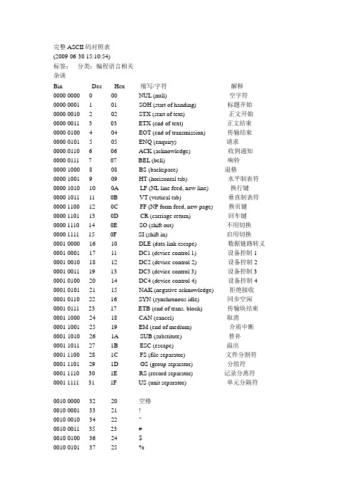
完整ASCII码对照表(2009-06-30 15:10:54)分类:编程语言相关标签:杂谈Bin Dec Hex 缩写/字符解释0000 0000 0 00 NUL (null) 空字符0000 0001 1 01 SOH (start of handing) 标题开始0000 0010 2 02 STX (start of text) 正文开始0000 0011 3 03 ETX (end of text) 正文结束0000 0100 4 04 EOT (end of transmission) 传输结束0000 0101 5 05 ENQ (enquiry) 请求0000 0110 6 06 ACK (acknowledge) 收到通知0000 0111 7 07 BEL (bell) 响铃0000 1000 8 08 BS (backspace) 退格0000 1001 9 09 HT (horizontal tab) 水平制表符0000 1010 10 0A LF (NL line feed, new line) 换行键0000 1011 11 0B VT (vertical tab) 垂直制表符0000 1100 12 0C FF (NP form feed, new page) 换页键0000 1101 13 0D CR (carriage return) 回车键0000 1110 14 0E SO (shift out) 不用切换0000 1111 15 0F SI (shift in) 启用切换0001 0000 16 10 DLE (data link escape) 数据链路转义0001 0001 17 11 DC1 (device control 1) 设备控制1 0001 0010 18 12 DC2 (device control 2) 设备控制2 0001 0011 19 13 DC3 (device control 3) 设备控制3 0001 0100 20 14 DC4 (device control 4) 设备控制4 0001 0101 21 15 NAK (negative acknowledge) 拒绝接收0001 0110 22 16 SYN (synchronous idle) 同步空闲0001 0111 23 17 ETB (end of trans. block) 传输块结束0001 1000 24 18 CAN (cancel) 取消0001 1001 25 19 EM (end of medium) 介质中断0001 1010 26 1A SUB (substitute) 替补0001 1011 27 1B ESC (escape) 溢出0001 1100 28 1C FS (file separator) 文件分割符0001 1101 29 1D GS (group separator) 分组符0001 1110 30 1E RS (record separator) 记录分离符0001 1111 31 1F US (unit separator) 单元分隔符0010 0000 32 20 空格0010 0001 33 21 !0010 0010 34 22 "0010 0011 35 23 #0010 0100 36 24 $0010 0101 37 25 %0010 0111 39 27 ' 0010 1000 40 28 ( 0010 1001 41 29 ) 0010 1010 42 2A* 0010 1011 43 2B + 0010 1100 44 2C , 0010 1101 45 2D - 0010 1110 46 2E . 0010 1111 47 2F / 0011 0000 48 30 0 0011 0001 49 31 1 0011 0010 50 32 2 0011 0011 51 33 3 0011 0100 52 34 4 0011 0101 53 35 5 0011 0110 54 36 6 0011 0111 55 37 7 0011 1000 56 38 8 0011 1001 57 39 9 0011 1010 58 3A: 0011 1011 59 3B ; 0011 1100 60 3C < 0011 1101 61 3D = 0011 1110 62 3E > 0011 1111 63 3F ? 0100 0000 64 40 @0100 0001 65 41 A 0100 0010 66 42 B 0100 0011 67 43 C 0100 0100 68 44 D 0100 0101 69 45 E 0100 0110 70 46 F 0100 0111 71 47 G 0100 1000 72 48 H 0100 1001 73 49 I 0100 1010 74 4A J 0100 1011 75 4B K 0100 1100 76 4C L 0100 1101 77 4D M 0100 1110 78 4E N 0100 1111 79 4F O 0101 0000 80 50 P0101 0010 82 52 R 0101 0011 83 53 S 0101 0100 84 54 T 0101 0101 85 55 U 0101 0110 86 56 V 0101 0111 87 57 W 0101 1000 88 58 X 0101 1001 89 59 Y 0101 1010 90 5A Z 0101 1011 91 5B [ 0101 1100 92 5C \ 0101 1101 93 5D ] 0101 1110 94 5E ^ 0101 1111 95 5F _ 0110 0000 96 60 `0110 0001 97 61 a 0110 0010 98 62 b 0110 0011 99 63 c 0110 0100 100 64 d 0110 0101 101 65 e 0110 0110 102 66 f 0110 0111 103 67 g 0110 1000 104 68 h 0110 1001 105 69 i 0110 1010 106 6A j 0110 1011 107 6B k 0110 1100 108 6C l 0110 1101 109 6D m 0110 1110 110 6E n 0110 1111 111 6F o 0111 0000 112 70 p 0111 0001 113 71 q 0111 0010 114 72 r 0111 0011 115 73 s 0111 0100 116 74 t 0111 0101 117 75 u 0111 0110 118 76 v 0111 0111 119 77 w 0111 1000 120 78 x 0111 1001 121 79 y 0111 1010 122 7A z 0111 1011 123 7B {0111 1101 125 7D }0111 1110 126 7E ~0111 1111 127 7F DEL (delete) 删除NUL VT 垂直制表SYN 空转同步SOH 标题开始FF 走纸控制ETB 信息组传送结束STX 正文开始CR 回车CAN 作废ETX 正文结束SO 移位输出EM 纸尽EOY传输结束SI 移位输入SUB 换置ENQ 询问字符DLE 空格ESC 换码ACK 承认DC1 设备控制1 FS 文字分隔符BEL 报警DC2 设备控制2 GS 组分隔符BS 退一格DC3 设备控制3 RS 记录分隔符HT 横向列表DC4 设备控制4 US 单元分隔符LF 换行NAK 否定DEL 删除键盘常用ASCII码ESC键VK_ESCAPE (27)回车键:VK_RETURN (13)TAB键:VK_TAB (9)Caps Lock键:VK_CAPITAL (20)Shift键:VK_SHIFT ($10)Ctrl键:VK_CONTROL (17)Alt键:VK_MENU (18)空格键:VK_SPACE ($20/32)退格键:VK_BACK (8)左徽标键:VK_LWIN (91)右徽标键:VK_LWIN (92)鼠标右键快捷键:VK_APPS (93) Insert键:VK_INSERT (45) Home键:VK_HOME (36)Page Up:VK_PRIOR (33)PageDown:VK_NEXT (34)End键:VK_END (35)Delete键:VK_DELETE (46) 方向键(←):VK_LEFT (37)方向键(↑):VK_UP (38)方向键(→):VK_RIGHT (39)方向键(↓):VK_DOWN (40)F1键:VK_F1 (112)F2键:VK_F2 (113)F3键:VK_F3 (114)F4键:VK_F4 (115)F5键:VK_F5 (116)F6键:VK_F6 (117)F7键:VK_F7 (118)F8键:VK_F8 (119)F9键:VK_F9 (120)F10键:VK_F10 (121)F11键:VK_F11 (122)F12键:VK_F12 (123)Num Lock键:VK_NUMLOCK (144) 小键盘0:VK_NUMPAD0 (96)小键盘1:VK_NUMPAD0 (97)小键盘2:VK_NUMPAD0 (98)小键盘3:VK_NUMPAD0 (99)小键盘4:VK_NUMPAD0 (100)小键盘5:VK_NUMPAD0 (101)小键盘6:VK_NUMPAD0 (102)小键盘7:VK_NUMPAD0 (103)小键盘8:VK_NUMPAD0 (104)小键盘9:VK_NUMPAD0 (105)小键盘.:VK_DECIMAL (110)小键盘*:VK_MULTIPLY (106)小键盘:VK_MULTIPLY (107)小键盘-:VK_SUBTRACT (109)小键盘/:VK_DIVIDE (111)Pause Break键:VK_PAUSE (19) Scroll Lock键:VK_SCROLL (145)。
CEPA免关税货品清单

1
Serial No. 41 42 43 44 45 46 47 48 49 50 51 52 53 54 55 56 57 58 59 60 61 62 63 64 65 66 67 68 69 70 71 72 73 74 75 76 77 78 79 80 81 82 83 84 85
Mainland 2001 Tariff Codes 39269010 39269090 41041000 41043990 48051000 48056000 48058000 48101200 48102900 48109100 48119000 48191000 48192000 48211000 48239090 49111090 49119900 50072019 51071000 51121900 52051100 52051200 52052200 52053200 52054200 52083200 52083300 52083900 52084200 52084900 52091200 52093100 52093200 52093900 52094100 52094200 52094300 52103100 53091900 53092900 54011010 54074200 54074300 54075200 54076100
Parts of machines or instruments, of plastics Other articles of plastics Whole bovine skin leather, of a unit surface area not exceeding 2.6 square meter Other leather of bovine or equine animals Semi-chemical fluting paper (corrugating medium) Other thin uncoated paper and paperboard Other thick uncoated paper and paperboard Thick writing and printing paper and paperboard, coated with inorganic substance Other writing and printing paper and paperboard, coated with inorganic substance Multi-ply paper and paperboard, coated with inorganic substance Other coated, impregnated or covered paper and paperboard Cartons, boxes and cases, of corrugated paper or paperboard Folding cartons, boxes and cases, of non-corrugated paper or paperboard Printed paper or paperboard labels of all kinds Other paper and articles of paper Other trade advertising material and the like Other printed matters Other fabrics of bombyx mori silk Yarn of combed wool, not put up for retail sale Fabrics of combed wool, of a weight exceeding 200g/square meter Cotton single yarn, measuring high decitex, carded, not put up for retail sale Cotton single yarn, measuring medium decitex, carded, not put up for retail sale Cotton single yarn, measuring medium decitex, combed, not put up for retail sale Cotton multiple or cabled yarn, measuring medium decitex, carded, not put up for retail sale Cotton multiple or cabled yarn, measuring medium decitex, combed, not put up for retail sale Lighter weight plain weave cotton fabric, dyed Light weight 3-thread or 4-thread twill cotton fabric, dyed Other light weight cotton fabrics, dyed Light weight plain weave cotton fabric, of yarns of different colours Other light weight cotton fabrics, of yarns of different colours Heavy weight 3-thread or 4-thread twill cotton fabric, unbleached Heavy weight plain weave cotton fabric, dyed Heavy weight 3-thread or 4-thread twill cotton fabric, dyed Other heavy weight cotton fabrics, dyed Heavy weight plain weave cotton fabric, of yarns of different colours Heavy weight twill cotton fabric (denim), of yarns of different colours Heavy weight 3-thread or 4-thread twill cotton fabric, of yarns of different colours Light weight plain weave cotton fabric mixed with man-made fibres, dyed Other fabrics of mainly flax Other fabrics of flax, mixed with other textile materials Sewing thread of syntheor retail sale Fabrics of mainly nylon, dyed Fabrics of mainly nylon, of yarns of different colours Fabrics of mainly textured polyester filaments, dyed Other fabrics, of mainly non-textured polyester filaments
ASC编码对照表
055 056 057 058 059 060 061 062 063 064 065 066 067 068 069 070 071 072 073083 084 085 086 087 088 089 090 091 092 093 094 095 096 097 098 099 100 101 102 103 104 105 106 107 108 109 110 111 112 113 114 115 116 117 118 119
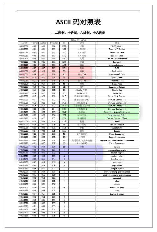
ASCII 码对照表
---二进制、十进制、八进制、十六进制
二进制 00000000 00000001 00000010 00000011 00000100 00000101 00000110 00000111 00001000 00001001 00001010 00001011 00001100 00001101 00001110 00001111 00010000 00010001 00010010 00010011 00010100 00010101 00010110 00010111 00011000 00011001 00011010 00011011 00011100 00011101 00011110 00011111 00100000 00100001 00100010 00100011 00100100 00100101 00100110 00100111 00101000 00101001 00101010 00101011 00101100 00101101 00101110 00101111 00110000 00110001 00110010 00110011 00110100 00110101 00110110 十进制 000 001 002 003 004 005 006 007 008 009 010 011 012 013 014 015 016 017 018 019 020 021 022 023 024 025 026 027 028 029 030 031 032 033 034 035 036 037 038 039 040 041 042 043 044 045 046 047 048 049 050 051 052 053 054 八进制 000 001 002 003 004 005 006 007 010 011 012 013 014 015 016 017 020 021 022 023 024 025 026 027 030 031 032 033 034 035 036 037 040 041 042 043 044 045 046 047 050 051 052 053 054 055 056 057 060 061 062 063 064 065 066 十六进制 000 001 002 003 004 005 006 007 008 009 00A 00B 00C 00D 00E 00F 010 011 012 013 014 015 016 017 018 019 01A 01B 01C 01D 01E 01F 020 021 022 023 024 025 026 027 028 029 02A 02B 02C 02D 02E 02F 030 031 032 033 034 035 036 值 NULL SOH STX ETX EOT ENQ ACK BEL BS HT LF VT FF CR SO SI DLE DC1 DC2 DC3 DC4 NAK SYN ETB CAN EM SUB ESC FS GS RS US SP ! " # $ % & ' ( ) * + , . / 0 1 2 3 4 5 6 ASCII 码,ASC2 说明 空值 标题开始 文本开始 文本结束 文尾 查询 确认 振铃 退格 横向 Tab 换行 竖向 Tab 换页 回车 Shift 弹起 Shift 按下 数据通讯交换码 设备控制 1(XON) 设备控制 2 设备控制 3(XOFF) 设备控制 4 不确认 同步空闲 取消传送 取消 媒体结束 替代 退出 文件分隔符 分组符 发送请求/ 记录分离符 单元分割符 空格 原文 Null char. Start of Header Start of Text End of Text End of Transmission Enquiry Acknowledgment Bell Backspace Horizontal Tab Line Feed Vertical Tab Form Feed Carriage Return Shift Out Shift In Data Link Escape Device Control 1 Device Control 2 Device Control 3 Device Control 4 Negative Acknowledgement Synchronous Idle End of Trans. Block Cancel End of Medium Substitute Escape File Separator Group Separator Request to Send/Record Separator Unit Separator Space exclamation mark double qopte number sign dorrlar sign percent ampersand single quote left/opening parenthesis right/closeing parenthesis asterisk plus comma minus or dash dot forward slash
Small degree representations of finite Chevalley groups in defining characteristic

Small degree representations offinite Chevalley groups in defining characteristicFrank L¨u beckAugust24,2000AbstractWe determine for all simple simply connected reductive linear algebraic groups defined over afinitefield all irreducible representations in their defining character-istic of degree below some bound.These also give the small degree projective rep-resentations in defining characteristic for the correspondingfinite simple groups.For large rank our bound is proportional to and for rank much higher.The small rank cases are based on extensive computer calculations.1IntroductionIn this note we give lists of projective representations of simple Chevalley groups in their defining characteristic.There are two types of results.First we determine for groups of rank all such representations of degree smaller or equal some bound depending on the type(e.g.,100000for type).In particular this contains a complement to the tables of representations in non-defining characteristic up to degree250given in[7].These data are produced using a collection of computer programs developed by the author.Then we determine for groups of classical type of rank all representations of degree at most for type,respectively for the other types.For large there is a small list and for small this range is easily covered by our tables mentioned above. This extends results by Kleidman and Liebeck[11,5.4.11].Wefix some notation for the whole paper.Let be afinite twisted or non-twisted simple Chevalley group in characteristic.There is an associated connected reductive simple algebraic group over of simply connected type,a Frobenius endomorphism of,a with and an such that:—is defined over via.—For the group of-fixed points with center we have.—is the quotient of the universal covering group of by the-part of its center.So,asking for the projective representations of in characteristic is the same as asking for the representations of in characteristic.These can be constructed by restricting certain representations,called highest weight representations,of the alge-braic group to.This is explained in Section2.In Section3we shortly describe how our computer programs for computing weight multiplicities work.In Section4we describe our main results consisting of lists of small degree representations for groups12Frank L¨u beckof rank at most11.The lists are printed in Appendix6.Finally,in Section5we consider groups of larger rank.Acknowledgements.I wish to thank Kay Magaard,Gunter Malle and Gerhard Hißfor useful discussions about the topic of this note.2Representations in defining characteristicThere are several well readable introductions to this topic,for example Humphreys’survey[9].A detailed reference is Jantzen’s book[10].We recall some of the basic facts.For of simply connected type of rank as in the introduction let be a maximal torus of,its character group and its co-character group.Let be a set of simple roots for this root system andthe coroot corresponding to,.Viewing as Euclidean space we define the fundamental weights as the dual basis of. This is a-basis of(because is simply connected).There is a partial ordering on defined by if and only if is a non-negative linear combination of simple roots.A weight is called dominant if it is a non-negative linear combination of the fundamental weights.The Weyl group of,generated by the reflections along the,acts on.Under this action each -orbit on contains a unique dominant weight.From now on let be afinite dimensional-module over.Considering this as-module there is a direct sum decomposition into weight spaces such that acts by multiplication with on.The set of with is called the set of weights of.The set of weights of is a union of -orbits and for,we have.The following basic results are due to Chevalley.Theorem2.1Let be as above.(a)If is irreducible then the set of weights of contains a(unique)element such that for all weights of we have.This is called the highest weight of ,it is dominant and we have.(b)An irreducible-module is determined up to isomorphism by its highest weight.(c)For each dominant weight there is an irreducible-module with highest weight.A dominant weight is called-restricted iffor.The following result of Steinberg shows how all highest weight modules of can be constructed out of those with-restricted highest weights.Theorem2.2(Steinberg’s tensor product theorem)Let be the Frobenius auto-morphism of,raising elements to their-th power.Twisting the-action on a -module with,,we get a new-module which we denote by.If are-restricted weights thenSmall degree representations in defining characteristic3 Finally we need to recall the relation between the irreducible modules of the alge-braic group and those of thefinite group.This is nicely described by Steinberg in[16,13.3,11.6].Theorem2.3Let and be as in the introduction.We define a subset of dom-inant weights.If is not a Suzuki or Ree group(i.e.,not of type,or )then for.In the case of Suzuki and Ree groups we defineif is a short root(note that is the square root of an odd power of or,respectively,in these cases).Then the restrictions of the-modules with to form a set of pairwise inequivalent representatives of all equivalence classes of irreducible-modules.These results show that the dimensions of the irreducible representations of the groups over are easy to obtain if we know the dimensions of the representa-tions of the algebraic groups for-restricted weights.3Computation of weight multiplicitiesIn this section we sketch how we compute the degree of the representation for given root datum of,highest weight and prime.For almost all it is the same as for the algebraic group over the complex numbers with same root datum,respectively its Lie algebra.In these cases the degree can be computed by a formula of Weyl,see[8, 24.3].In the other cases no formula is known.But in principle there is an algorithm to compute the degree.This is described in[8,Exercise2of26.4]and goes back to Burgoyne[2].This was also used in[6]to handle some cases in exceptional groups. The idea is to construct a so-called Weyl module generically over the integers. By base change this leads to a module for any with the given root datum over any ring,which has as a highest weight.Over or over for almost all this is irreducible and so isomorphic to.In general is a quotient of.To construct one considers the universal enveloping algebra of the com-plex Lie algebra corresponding to the given root datum.It contains a-lattice,the Kostant-form of,which is defined via a Chevalley basis of the Lie algebra.Up to equivalence there is a unique irreducible highest weight representation for with highest weight.Let be a vector of weight(this is unique up to scalar).Then we set.Wefix an ordering of the set of positive roots.Then and have -bases labeled by sequences of non-negative integers.Applying such a basis element of to a vector of weight we get a vector of weight(and similarly for basis vectors of).So,decomposingaccording to the weight spaces,we can describe generating sets of by all non-negative linear combinations of positive roots which are equal to.There is a non-degenerate bilinear form on which can be described via this generating system.Different weight spaces are orthogonal with respect to this form.Let be two coefficient vectors as above such that the corresponding linear combination of the positive roots is the same.Then is again of weight and one defines.4Frank L¨u beckSince the form is nondegenerate we can compute the rank of a weight latticeby computing the rank of the matrix where and are running through all non-negative linear combinations of positive roots for.The dimension of the weight space of is the rank of modulo.The coefficients can be computed by simplifying the element with the help of the commutator relations in,see[8,25.].These involve the structure con-stants for a Chevalley basis of the corresponding Lie algebra which can be computed as described in[3,4.2].In principle this allows the determination of for all,and.But in practice these computations can become very long,already in small examples.There are technical problems like the question how to apply commutator relations most effi-ciently in order to compute the integers.Different strategies change the number of steps in the calculation considerably.But the main problem is that the generating sets for the weight spaces as described above are very ually the number of non-negative linear combinations of positive roots which yield is much larger than the dimension of.By a careful choice of the ordering of the positive roots one can reduce the linear combinations to consider,because for manywith there is a such thatis not a weight of(and hence).But the main improvement we get by using results of Jantzen and Andersen, see[10,II.8.19].The so-called Jantzen sum formula expresses the determinant of the Gram matrix of the bilinear form on the lattice in terms of weight multi-plicities of various with.The weight multiplicities of these can be efficiently computed by Freudenthal’s formula,see[8,22.3].In particular the formula gives exactly the set of primes for which the Weyl module is not isomorphic to .In rare cases it happens that a prime divides such a determinant exactly once-then we know without further calculations that.Using these determinants we compute only parts of the matrices correspond-ing to a subset of its rows and columns until the submatrix has the full rankand the product of its elementary divisors is equal to the known determinant.Then clearly the rank of modulo is the same as the rank of this submatrix modulo.With this approach we never need submatrices of of much larger dimension than.(In[6]the consideration of the matrices was substituted by com-puting somewhat smaller matrices using the action of parabolic subalgebras in cases where has a non-trivial stabilizer in,but these matrices were still big compared to the dimension of the weight spaces.)Of course,our method is limited to representa-tions where no single weight space has a dimension of more than a few thousand.Actually we can also compute by our approach the Jantzenfiltrations of the Weyl modules,see[10,II.8],since we compute the elementary divisors of the matrices and not just their rank.To do this one also needs a sophisticated algorithm to compute the exact elementary divisors of Gram matrices of this size.We developed the algorithm described in see[12]for this purpose.We have a collection of computer programs for doing the calculations described above,which are based on the computer algebra system GAP[14]and the package CHEVIE[5].They are currently in a usable but still experimental state.It is planned to improve their efficiency,to extend their functionality and to put this into a package which will be made available to other users.We postpone a much more detailed version of this very sketchy section until this package is ready.Small degree representations in defining characteristic5 4Representations of small degree for groups of small rankFrom Theorem2.2we see how to construct any highest weight representationof from those with-restricted weights by twisting withfield automorphisms and tensoring.Assume now we are given the type of an irreducible root system and a number .We consider the groups over with this root system for all at once.We want tofind for all primes all-restricted dominant weights such that the highest weight representation of the group over has degree smaller or equal.Our main tool to restrict this question to afinite number of to consider is the following result by Premet,see[13].Recall from Section2that the set of weights of is a union of-orbits and that each-orbit contains a unique representative which is dominant.Theorem4.1If the root system of has different root lengths we assume thatand if is of type we also assume.Then the set of weights of is the union of the-orbits of dominant weights with.The length of the-orbit of a dominant weight is easy to compute by the following remark,see[8,10.3B]for a proof.Remark4.2Let be a dominant weight.Then the stabilizer in the Weyl group of is the parabolic subgroup generated by the reflections along the simple roots for which.Here is an algorithm forfinding a set of candidate highest weights for representa-tions of of rank at most a given bound.Algorithm4.3Input:An irreducible root system and an.Output:A set of dominant weights which contains all such that there is a prime with-restricted and a group over corresponding to the given root system with highest weight representation of degree at most.—To handle the exceptions in Premet’s theorem we put all-,respectively-restricted weights into,if the root system has roots of different lengths.—If not yet considered we compute for all-restricted weights a lower bound for the dimension of for any corresponding by counting the number of its weights (using4.1and4.2).If the bound is at most we put this weight into.—We choose a linear function which takes positive values on the simple roots,(and hence on the fundamental weights).Then we determine recursively all dominant weights with growing value of and compute for them a lower bound for as above.If it is at most we put the weight into. We proceed until wefind an interval such that for all and such that for all dominant with the dimension of is bigger than.Proof.We show that all with have dimension for any:This is clear for which were considered during the algorithm.Thosewhich were not considered are not-restricted and so one coefficient.But then is also a dominant weight(an expression of as linear combination6Frank L¨u beckof the fundamental weights is given by the-th column of the Cartan matrix of theroot system of,this matrix contains’s on the diagonal and non-positive numberselsewhere).We have.Repeating this step recursively for the smaller weight we must eventuallyfind a dominant weight which is-restrictedand not in or for which.Since the orbit lengths of dominant weights already sum up to more than the same holds for.The algorithm stops since for any given bound there are onlyfinitely many dominant weights with less than smaller dominant weights.(If a coefficient of as above is bigger than,,then we have seen that are also dominant for.)In Table1wefix some bound for each irreducible root system of rank at most,respectively in case.Table1:MMType3007001000200040005000700080001000012000 MType200030004000500010000150001800020000 MFor each irreducible root system with rank at most11we used the defined aboveas input for Algorithm4.3.For each weight in the output set and for all primes for which is-restricted we computed the exact weight multiplicities of using the techniques described in Section3.Actually we stopped such a computation whenever we found that thefinal dimension will be larger than.The bounds were chosen such that the results presented below could be com-puted interactively with our programs within about two days using10computers in parallel.The types,,were added upon request of Gunter Malle,who asked to cover in this note all representations of degree for a specific application.Here is our main result.Theorem4.4For any type of root system and number as given in Table1and all primes the Tables6.5to6.52list the-restricted weights such that the representa-tion of the algebraic group over has degree at most.The exact degree of is also given.Furthermore we describe the centers of the groups and the action of the fundamental weights on the center in6.2.This allows to determine the kernels of the representations.The Frobenius-Schur indicators in case are given by6.3.As mentioned above we have actually computed the exact weight multiplicities for the representations appearing in the tables of Section6.It would take too much space to print this in detail but the results are available upon request from the author.Small degree representations in defining characteristic7 The types considered above do not include,i.e.,.The reason is that this case is easy to describe systematically.This seems to be well known but also follows immediately from4.1since all weight multiplicities are at most in this case, see[8,7.2].Remark4.5If is of type then the representation with has degree.For odd the center of is non-trivial and of order.It is contained in the kernel of if and only if is even.5Representations of small degree for groups of large rankIn this section we consider classical groups of large rank.We prove the following result.Theorem5.1Let be of classical type and be the rank of.Set if is of type and otherwise.If then all-restricted weights such that the highest weight representation of has dimension at most are given in the following table.The table also includes the dimensions of these modules.(Note that the case of type and is included in case and.)The fundamental weights are labeled as explained in6.1.type,all,allallallallallNote that the corresponding result for of rank is included in Theorem4.4.8Frank L¨u beckProof.Wefirst prove that the weights which don’t appear in our table correspond to representations of degree larger than.(Case,)Let be a dominant weight.If somethen the-stabilizer of is contained in a reflection subgroup of type, see4.2.Hence,the-orbit of and so is at leastFor and we have.If and then the stabilizer of is contained in a reflection group of type,whose index is for all.This shows that only weights with at most one non-zero coefficient,either or ,can appear in our list.If then,as explained in the proof of4.3,is also a dominant weight.But this has coefficient ing the estimate as above for this smaller weight and Premet’s theorem4.1(note that the considered now is not-restricted)we see again that.A similar argument shows that for weights in our list.So,the only weights which could(and actually do)lead to degrees are,, and.(Case)Here wefind the relevant with very similar arguments as in case and.(Case)Because of the symmetry of the Dynkin diagram the weights and must describe representations of equal degree(in fact they are dual to each other).We can again use very similar arguments as above tofind the relevant weights for our list.(Here we rule out andby observing.)It remains to determine the exact degrees of the in our table.Probably they are known to the experts but we could notfind references for all cases.Type and and for the other types are contained in[11,5.4.11]and[8,25.5,Ex.8].We include a proof for the degrees of and in types,and following hints of K.Magaard and G.Hiß.The idea is to use explicit modules.For all types we know the-modules ,.These are the natural modules of, ,or,respectively.We determine the constituents offor.Note that for these types is self-dual.Since the caseis covered by the references above(is not-restricted),we assume in the rest of the proof that is odd.We will use the following general remarks.If is an indecomposable-module then has the trivial module as direct summand if and only if(here denotes the dual module).In that case there is exactly one trivial direct summand, see[1,3.1.9]for a proof.If is a basis of then has two submodules with basisand with basis.Since we have.(Case)Let,be a basis of the natural symplectic module such that for the symplectic form we have,and for all.Then the vectoris invariant under the symplectic group.If this vector must span the unique trivial direct summand mentioned above.Small degree representations in defining characteristic9 The group contains a subgroup isomorphic to.An element acts on the subspace of spanned by and by its inverse on the subspace spanned by.Hence restricted to this subgroup is isomorphic to.Restricting the representation to this subgroup we find the decomposition, see[4,I,12.].Using the known degrees for case,we see that this contains at most trivial constituents.The similar restriction to a subgroup of type shows by induction that one irreducible constituent of has degree at least .Comparing degrees we see that the three non-trivial constituents in the restriction to must lie in a single constituent of.To summarize,we have at most one non-trivial and two trivial constituents.If there are trivial constituents then one must be in the sockle,i.e.,there must be an invariant vector.This can only be the one we see in the-summand of the restriction to.We can write down such a vector and check that it is not invariant under the whole group ,apply an element which does not leave the space spanned by invariant. We have proved that is irreducible.We can argue very similarly for.If wefind that it is a direct sum of an irreducible and the trivial module found above.If wefind that there is one non-trivial constituent,exactly one trivial constituent in the sockle and at most two trivial constituents.Since in this case the trivial constituent in the sockle is not a direct summand there must be a second trivial constituent in the head,by duality.If has a highest weight vector then is contained in and has weight.Hence.The other constituents of the tensor product must correspond to dominant weights smaller than,there are only two of them,and.We get that the non-trivial constituent of is isomorphic to.(Case)This can be handled by almost exactly the same arguments as the case .Here the trivial submodule is contained in.(Case)In this case we consider the restrictions of to subgroups of type,.This leads to decompositions.Comparing this decomposition for and or,respectively,and using the results for type and in-duction we see as in type that has only one non-trivial and maybe a few trivial constituents.There is an such that and.The decomposition above for this shows that there are at most two trivial constituents.Furthermore,as in type wefind a trivial submodule.Either this is a direct summand(if)then it is the only trivial constituent or otherwise there is a second constituent in the head of .The argument for is again very similar.Thisfinishes the proof.It would be interesting if the degrees in our list could be determined more sys-tematically in the framework of highest weight modules.Then one could work out systematically generalizations of Theorem5.1where the bound is substituted by anyfixed polynomial in.Checking that the statement in Theorem5.1is also true for of type and ,we get the following Corollary.This completes the list in[7]which gives all representations of in non-defining characteristic of degree at most.Corollary5.2For any simple over wefind all-restricted weights of such that has degree in the tables given in Theorems4.4and5.1.10Frank L¨u beck6Appendix:Tables for groups of rank at most 11In this section we give the detailed lists for Theorem 4.4.We start by introducing some notation and describe the centers of the groups and the action of the fundamental weights on the center.6.1Ordering of fundamental weightsFor the irreducible types of root systems we choose the following ordering for thesimple roots ,the corresponding corootsand the fundamental weights ,.(We show the Dynkin diagrams with the node of labeled by .)14571457214145432126.2Action of fundamental weights on the center ofWe give for each irreducible type of root system the values of for in the center of .To compute this we use that is contained in a maximal torus of .Such a is isomorphic to and consists of those withfor all .So,we have to solve a system of equations given by the Cartan matrix of the root system.We denote an element whose multiplicative order is .For we write for the maximal divisor of prime to .For elements we write.is cyclic of order .For the generator we have(,odd)is cyclic of order for odd and for .There is a generator such that(,even)is elementary abelian of order with if is odd and if.There are generators and such that.Here is the element such that.()is cyclic of order if and if.There is a generator such that.()is trivial.6.3Frobenius-Schur indicatorsIf is odd we can determine the Frobenius-Schur indicators of the representations in our lists using a result of Steinberg,see[15,Lemmas78and79].If is of type or of type with odd or of type then the representations and,where the permutation is given by the auto-morphism of order two of the Dynkin diagram,are dual to each other.For other all are self-dual.If is self-dual(and recall that is odd)then its Frobenius-Schur indicator is ‘+’if has no element of order.Otherwise it is the sign of where is the only element of order in,respectively in case with even.This can be computed by6.2.6.4An exampleAs an example how to read the data in this Appendix,let us determine all irreducible representations in defining characteristic for groups of type Spin, which have degree:We apply Theorems2.2and2.3.Wefirst need to compute all factorizations of into factors which appear as degrees in6.22.Although many divisors of appear as degree the only factorization is.Now we have a closer look at6.22.If then there is no irreducible representation of degree.And the listed representations of degree do not correspond to-restricted weights.So,in charac-teristic there are no irreducible representations of this degree.The same conclusion holds for.In this case there is no irreducible represen-tation of degree.If there is of degree and of degree.Ifwefind for any,,the irreducible representationrestricted to of degree.Furthermore we see in6.22 that and have degree.For larger there is no representation of degree in our list.We onlyfindand in case also.In all cases where we have found representations is odd and so the center of and of is of ing6.2we see that for the non-trivial element in the center we have and for.Applying this to the representations found above wefind that only in case is not faithful.From6.3we see that this is also the only representation with Frobenius-Schur indicator‘+’.The others have indicator‘-’.In type the representations andare dual to each other,in particular they have the same dimension.In6.5to6.20we save some space by only including one of such a pair of representations.6.5Case,(Recall the remark before6.5.)deg deg deg6.6Case,(Recall the remark before6.5.)deg deg deg6.7Case,(Recall the remark before6.5.)deg deg deg6.8Case,(Recall the remark before6.5.)deg deg deg6.9Case,(Recall the remark before6.5.)deg deg deg6.10Case,(Recall the remark before6.5.)deg deg deg1(00000000)all966(00010001)22079(10000011)2,3,59(00000001)all966(00010001)32304(00001100)336(00000010)all990(00000012)all2352(00001010)245(00000002)all1008(00001001)52385(00100010)379(10000001)31050(00010001)2,32394(00100010)280(10000001)31135(01000010)72520(00000200)384(00000100)all1214(01000010)22691(00100010)7 126(00001000)all1215(01000010)2,72700(00100010)2,3,7 156(00000011)31278(00000013)52772(00000102)5 165(00000003)all1287(00000005)all2844(00000021)3 240(00000011)31359(10000011)32907(00002000)3 306(01000001)21395(10000003)112922(00000022)5 315(01000001)21440(10000003)112970(00000021)3 387(10000002)51461(01000002)33003(00000006)all 396(10000002)51540(01000002)33060(00010010)5 414(00000020)31554(00000200)33139(00011000)3 495(00000004)all1764(00000110)23168(00000013)5 504(00000101)21864(20000002)113318(00001010)5 540(00000020)31890(00000102)53402(00001010)2,5 630(00000101)21890(00000110)2,33414(02000001)3 684(00100001)71943(20000002)53465(00100002)all 720(00100001)71944(20000002)5,113654(00001002)3 882(00000110)32034(10000011)23744(00010010)3 882(00001001)52043(10000011)53780(00010010)3,5。
2006年监管证件名称代码表说明

2006年监管证件名称代码表说明第一篇:2006年监管证件名称代码表说明2006年监管证件名称代码表说明一、监管证件名称代码监管证件名称代码,是海关依据我国外贸法律、法规及规章,为便于实施计算机系统管理和便捷通关需求,对实行进出口许可证件管理的货物在海关通关环节须验核的各种进出口许可证件的分类标识。
监管证件代码监管证件名称1----进口许可证2----两用物项和技术进口许可证3----两用物项和技术出口许可证4----出口许可证5----纺织品临时出口许可证6----旧机电产品禁止进口7----自动进口许可证8----禁止出口商品9----禁止进口商品A----入境货物通关单B----出境货物通关单D----出/入境货物通关单(毛坯钻石用)E----濒危物种出口允许证F----濒危物种进口允许证G----两用物项和技术出口许可证(定向)I----精神药物进(出)口准许证J----金产品出口证或人总行进口批件O----自动进口许可证(新旧机电产品)P----进口废物批准证书Q----进口药品通关单S----进出口农药登记证明T----银行调运外币现钞进出境许可证W----麻醉药品进出口准许证X----有毒化学品环境管理放行通知单Y----原产地证明Z----进口音像制品批准单或节目提取单a----请审查预核签章e----关税配额优惠税率进口棉花配额证s----适用ITA税率的商品用途认定证明t----关税配额证明r----预归类标志u----进口许可证(加工贸易,保税)x----出口许可证(加工贸易)y----出口许可证(边境小额贸易)二、监管证件名称代码简要说明(一)代码“1”----进口许可证:指商务部配额许可证事务局或其授权机关签发的进口许可证。
(二)代码“2”----两用物项和技术进口许可证:指列入《两用物项和技术进口许可证管理目录》的商品,进口时由商务部签发的《两用物项和技术进口许可证》。
1-s2.0-S0146638012000599-main
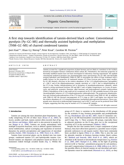
A first step towards identification of tannin-derived black carbon:Conventional pyrolysis (Py–GC–MS)and thermally assisted hydrolysis and methylation (THM–GC–MS)of charred condensed tanninsJoeri Kaal a ,⇑,Klaas G.J.Nierop b ,Peter Kraal c ,Caroline M.Preston daInstituto de Ciencias del Patrimonio (Incipit),Consejo Superior de Investigaciones Científicas (CSIC),San Roque 2,15704Santiago de Compostela,Spain bDepartment of Earth Sciences –Organic Geochemistry,Faculty of Geosciences,Utrecht University,P.O.Box 80021,3508TA Utrecht,The Netherlands cSouthern Cross GeoScience,Southern Cross University,P.O.Box 157,Lismore,2480New South Wales,Australia dPacific Forestry Centre,Natural Resources Canada,506West Burnside Rd.,Victoria,BC,Canada V8Z 1M5a r t i c l e i n f o Article history:Received 5October 2011Received in revised form 13March 2012Accepted 26March 2012Available online 5April 2012a b s t r a c tTannins account for a significant proportion of plant biomass and are likely to contribute to the residues formed by incomplete biomass combustion (black carbon,BC).Nonetheless,the molecular properties of thermally modified tannins have not been investigated in laboratory charring experiments.We applied conventional analytical pyrolysis–gas chromatography–mass spectrometry (Py–GC–MS)and thermally assisted hydrolysis and methylation (THM–GC–MS)to investigate the effects of heat treatment with a muffle furnace on the properties of condensed tannins (CT)from Corsican pine (Pinus nigra )needles.Py–GC–MS showed a decrease in the relative abundance of the 1,2,3-trihydroxybenzenes (pyrogallols)at P 300°C and of the dihydroxybenzenes (mainly catechols)at P 350°C due to dehydroxylation of the CT B ring.Further dehydroxylation led to formation of monohydroxybenzenes (phenols),which showed a strong enrichment between 350and 400°C and,at higher temperatures,to a series of mono-cyclic and polycyclic aromatics [benzene,alkyl benzenes and polycondensed aromatic hydrocarbons (PAHs)].Degradation of the A ring could not be recognized via Py–GC–MS,probably because of the poor chromatographic behavior of 1,3,5-trihydroxybenzenes (phloroglucinols).The progressive dehydroxyla-tion and eventual polycondensation of the CT B ring was corroborated using THM–GC–MS.In addition,with THM–GC–MS the thermal rearrangement of CT A rings at 300°C and higher was inferred from the relative abundance of 1,3,5-trimethoxybenzenes (methylated phloroglucinol derivatives).These com-pounds were observed at moderate/high temperature (up to 450°C)and can not be produced from THM of lignin,suggesting that they may be markers of CT in natural BC samples.Ó2012Elsevier Ltd.All rights reserved.1.IntroductionTannins are among the most abundant plant biopolymers,typ-ically comprising 10–25%of foliar mass (Kraus et al.,2003).In leaves,needles and bark,tannin content often exceeds that of lig-nin (Hernes and Hedges,2004)and it is also present in woody tis-sue (Rogge et al.,1998).Tannins are strong antioxidants with multiple ecosystem functions,such as defense against herbivores,metal mobilization,radical scavenging and regulation of nutrient dynamics by protein precipitation and suppression of microbial activity (Zucker,1983;Kennedy et al.,1996;Fierer et al.,2001).Tannins from terrestrial plants can be divided into two main groups:condensed tannins (CT)and hydrolyzable tannins.Con-densed tannins are oligomers and polymers based on flavan-3-ol monomers linked through covalent bonds (Fig.1).Within thegroup of CT,there is variation in the distribution of OH groups on the aromatic B ring,forming procyanidin and prodelphinidin CT (e.g.Khanbabaee and van Ree,2001).Each CT monomer con-tains up to six OH functionalities concentrated on the aromatic A and B rings (Fig.1).These aromatic OH groups,especially those in adjacent positions on the B ring,give rise to the exceptional reactivity of CT in the environment (Slabbert,1992).Despite the fact that tannins form a major component of plant biomass,they have often been ignored as a possible source of poly-phenolic substances in soil organic matter;these have commonly been ascribed to lignin (Filley et al.,2006).This is also the case for phenolic moieties in biomass burning residue (black carbon,BC)(Baldock and Smernik,2002;Krull et al.,2003),which are abundant in BC formed at low/moderate temperature (e.g.Knicker et al.,2005,2007;Rumpel et al.,2006).In the light of growing interest in BC or ‘biochar’,amendment programs for soil ameliora-tion and C sequestration (Lehmann et al.,2006;Jeffery et al.,2011),the possible effects of charred tannins on soil microbial and nutri-ent dynamics must be understood (Warnock et al.,2010),as they0146-6380/$-see front matter Ó2012Elsevier Ltd.All rights reserved./10.1016/geochem.2012.03.009Corresponding author.Tel.:+34881813588;fax:+34881813601.E-mail address:joeri.kaal@incipit.csic.es (J.Kaal).may be anticipated to be vastly different from that of charred lig-nin.This is not possible,however,as methodologies for identifying charred tannins are not available and the thermal degradation pathways of tannins are largely unknown.The thermal alteration of plant tissue has been investigated in numerous studies,as reviewed by e.g.González-Pérez et al.(2004)and Preston and Schmidt (2006).Pyrolysis–gas chromatog-raphy–mass spectrometry (Py–GC–MS)is one method that can provide information on the molecular properties of BC (De la Rosa et al.,2008;Kaal and Rumpel,2009;Kaal et al.,2009;Fabbri et al.,2012),despite the fact that pyrolysis itself is a heat-induced scission reaction and that secondary rearrangements generate structures that may resemble the pyrolysis products of BC (Saiz-Jiménez,1994;Wampler,1999).Pyrolysis is a relatively inex-pensive and rapid technique that has also proven of value for tan-nin characterization (Galletti et al.,1995).Flash heating in the presence of tetramethylammonium hydroxide (TMAH)is referred to as thermally assisted hydrolysis and methylation (THM)or ther-mochemolysis.With THM,hydrolyzable bonds are cleaved and the resulting CO 2H and OH groups are transformed in situ to the corre-sponding methyl esters and methyl ethers,respectively (Challinor,2001;Hatcher et al.,2001;Shadkami and Helleur,2010),which are more amenable to GC than their underivatized counterparts.As such,THM–GC–MS provides additional information on tannin structure through detection of derivatized polyfunctionalized A and B rings (Nierop et al.,2005).In the present study the thermal degradation of CT was studied using laboratory charring experiments followed by characteriza-tion with Py–GC–MS and THM–GC–MS.The aim was to provide guidelines for the identification of CT-derived BC and identify the molecular changes as a function of charring temperature.2.Material and methodsCondensed tannins were isolated from Corsican pine (Pinus ni-gra var.maritima )needles from the coastal dunes in The Nether-lands (52°2004500N,4°3105700E)using the scheme proposed by Preston (1999)and described in detail by Nierop et al.(2005,2006).The CT were completely isolated from other components and had a prodelphinidin:procyanidin ratio of 2:1and average chain length of 6.6(Nierop et al.,2005).It has been used in various studies (Kaal et al.,2005;Nierop et al.,2006;Kraal et al.,2009).For the charring experiments,ca.200mg of CT were double wrapped in Al foil to simulate limited O 2availability during wild-fires.The samples were placed (30min)in a preheated muffle fur-nace at temperatures (T CHAR )from 200°C to 600°C.Similar experiments have been performed by Turney et al.(2006),Hall et al.(2008)and Wiesenberg et al.(2009).Weight loss was deter-mined gravimetrically before and after charring.C and H contents were determined by way of combustion using a LECO carbon ana-lyzer (model CHN-1000).Uncharred CT was used as a control.Py–GC–MS was performed in duplicate using a Pt filament coil probe Pyroprobe 5000pyrolyzer (CDS Analytical,Oxford,USA).Approximately 1–1.5mg sample was embedded in quartz tubes using glass wool.Pyrolysis was applied at 750°C for 10s (heating rate 10°C/ms).The method produces limited artificial charring during pyrolysis and a relatively high proportion of pyrolyzable biomass in comparison with pyrolysis at lower temperatures (Pastorova et al.,1994;Kaal et al.,2009;Song and Peng,2010).The pyrolysis interface was coupled to a 6890N GC instrument and 5975MSD (Agilent Technologies,Palo Alto,USA).The pyrolysis interface and GC inlet (split ratio 1:20)were set at 325°C.The GC instrument was equipped with a (non-polar)HP-5MS 5%phenyl,95%dimethylpolysiloxane column (30m Â0.25mm i.d.;film thickness 0.25l m)and He was the carrier gas (constant flow 1ml/min).The GC oven was heated from 50to 325°C (held 10min)at 20°C/min.The GC–MS transfer line was held at 270°C,the ion source (electron impact mode,70eV)at 230°C and the quadrupole detector at 150°C scanning a range between m /z 50and 500.Peak areas of the pyrolysis products were obtained from one or two characteristic or dominant fragment ions,the sum of which (total quantified peak area;TQPA)was set as 100%.Relative contributions of the pyrolysis products were calculated as %of TQPA.This is a semi-quantitative exercise that allows better comparison between samples than visual inspection of pyrolysis chromatograms alone.Benzofuran and styrene could not be quantified because of co-elution with contaminants.For THM–GC–MS,samples were pressed onto Curie-Point wires,after which a droplet of a 25%solution of TMAH in water was added,prior to drying under a 100W halogen lamp.THM was car-ried out using a Horizon Instruments Curie-Point pyrolyzer.Sam-ples were heated for 5s at 600°C.The pyrolysis unit was connected to a Carlo Erba GC8060furnished with a fused silica col-umn (Varian,25m Â0.25mm i.d.)coated with CP-Sil 5(film thick-ness 0.40l m).He was the carrier gas.The oven temperature program was:40°C (1min)to 200°C at 7°C/min and then to 320°C (held 5min)at 20°C/min.The column was coupled to a Fi-sons MD800MS instrument (m /z 45–650,ionization energy 70eV,cycle time 0.7s).Like Py–GC–MS,the relative contributions of the THM products were calculated as relative contributions to TQPA using 1–2dominant fragment ions.Benzene and toluene were not detected because they co-eluted with trimethylamine,the main side product of TMAH-based THM (Challinor,2001),i.e.with-in the solvent delay period (3min).Py–GC–MS and THM–GC–MS results were analyzed via princi-pal component analysis (PCA)to illustrate the major effects of heating on the pyrolysis and THM fingerprints,respectively,using SPSS 13.0.3.Results and discussion3.1.Weight loss and elemental compositionWeight loss from CT increased from 17%at T CHAR 200°C towards 56%at T CHAR 600°C (Table 1).The CT C content increased from 51%to 81%with increasing T CHAR .The atomic H/C ratio of the samples declined from 1.2to 0.6with increasing T CHAR ,reflecting loss of functional groups and formation of fused aromatic clusters through condensation (Braadbaart et al.,2004).Model structure of a condensed tannin oligomer;procyanidin,prodelphinidin,R =OH.47(2012)99–108chromatograms of uncharred(control)and charred(200–600°C)CT,from Py–GC–MS.Relative peak intensity vs.retention time3.2.Charred condensed tannin composition:Py–GC–MSPy–GC–MS total ion chromatograms are depicted in Fig.2.Total quantified peak area (Table 1),a rough measure of signal intensity,decreased with increasing T CHAR .This can be explained by the for-mation of non-pyrolyzable structures upon charring,probably through the formation of polycondensed aromatic clusters stable under pyrolysis conditions.However,this does not imply that the results from the high temperature chars should be dismissed for representing only a small and relatively volatilefraction:a more appropriate interpretation is that the samples consist largely of non-pyrolyzable fused aromatic clusters,corroborated by the dom-inant pyrolysis products of such samples (benzene and PAHs;see below)and lack of pyrolysis products from less intensely charred structures.The major pyrolysis products are listed in sponding retention times,fragment ions used and relative proportions.Products were structure,in particular the hydroxylation between benzenes (benzene and alkyl (with one OH),dihydroxybenzenes (DHB),(THB)and other compounds.The DHB are while the THB are based on pyrogallol moieties exclusively from prodelphinidin B rings.The uncharred CT isolate produced mainly pyrolysis (Table 2;Fig.3),which originate from prodelphinidin B rings,respectively.In contrast delphinidin:procyanidin ratio determined et al.,2005),the DHB were more abundant may be explained by way of the poor ‘‘visibility’’a non-polar GC column.The high proportion of and 4-methylpyrogallol points to scission of the the heterocyclic pyran C ring (Fig.1),which has sociation energy than the aromatic A and B acetone and acetic acid may represent the after pyrolysis.Products from the A ring were may be explained by the poor chromatographic rivatized 1,3,5-trihydroxybenzene principal pyrolysis product from the A ring (The lack of unambiguous A ring markers implies that Py–GC–MS cannot be used to study the degradation of the predominantly C-4/C-8and C-4/C-6intermonomeric linkages (Fig.1),and thus to investigate CT depolymerization.Some methoxyphenols (guaiacol and 4-vinylguaiacol)and catechol carbonate were detected.The guaiacols are commonly attributed to lignin and its derivatives (e.g.Kögel-Knabner,2002),but here they might alternatively orig-inate from C ring fission in CT (Galletti et al.,1995).The possibility of tannins as a source of the guaiacols is supported by the absence of resonances from methoxyphenols in liquid-state 13C NMR tra (Nierop et al.,2005)and guaiacols bearing a C 3side chain pyrolyzate,which should be detectable if residual lignin was ent in the fresh needle isolate (Saiz-Jiménez and de Leeuw,The results for uncharred CT were in good agreement with earlier pyrolysis experiments with tannin,catechin and gallocate-Relative proportion (TQPA)of pyrolysis product groups from CT vs.charring temperature (200–600°C);0°C,control (uncharred CT);THB,trihydroxybenzene;dihydroxybenzene;PAH,polycyclic aromatic hydrocarbon.Error bars reflect standard error of mean of two replicates.Note differences in y -axis scaling.Pyrolysis products plotted in PC1–PC2space (PCA).THB,trihydroxybenzene;dihydroxybenzene;PAH,polycyclic aromatic hydrocarbon.Arrow indicates trend in pyrolysis patterns with increasing charring temperature.The sample charred at200°C gave a pyrogram similar to that of uncharred CT,indicating limited thermal rearrangement at this temperature(Fig.2).At T CHAR300°C,the proportion of THB de-creased from ca.20%to ca.5%of the TQPA,while the proportion of DHB increased towards ca.70%(Fig.3).This reflects elimination of one OH from the prodelphinidin B ring during charring,causing a relative increase in the contribution of DHB to the pyrolyzate. Thus,the presence of DHB in pyrolyzates does not necessarily indi-cate the presence of uncharred CT.This sheds new light on results from previous studies(Quénéa et al.,2005a,b)in which the pres-ence of DHB in the pyrolyzate of BC-containing forest soil was interpreted as being from uncharred CT,whereas it may alterna-tively originate from CT-derived BC.A more drastic shift in pyro-lyzate composition occurred at T CHAR350°C:the relative abundance of DHB diminished,with a concomitant increase in phenols(from ca.10%to50%),as well as benzenes,PAH and other compounds(Fig.3).Also,the relative contribution of THB de-creased further.The results are indicative of strong B ring dehydr-oxylation at350°C.At T CHAR400°C,a further decrease in DHB contribution and increased relative abundance of benzenes and PAH were observed.The high biphenyl/naphthalene ratio may be specific for the pyrolyzate of CT-derived BC,as it is usually much lower in the pyrolyzate of char obtained from lignocellulose(Kaal et al.,2009).At T CHAR450°C,phenols decreased while the relative abundance of benzenes increased towards60%and that of PAHs to-wards10%,suggesting the loss of most of the OH groups from theB Fig.5.Total ion chromatograms of uncharred(control)and charred(200–600°C)CT,from THM–GC–MS.ring.The relatively weak signal for this sample (Table 1;Fig.2)sug-gested that a significant proportion of the CT was converted to non-pyrolyzable polycondensed aromatics.After charring at 600°C the phenolic pyrolysis products and the possible products of the C ring (acetylacetone,acetone and acetic acid)were absent,while the benzenes and PAH had increased to 75%and 20%,respec-tively (Fig.3).This combination constitutes a typical set of pyroly-sis products from strongly charred biomass (Kaal et al.,2009;Fabbri et al.,2012).The general trends for experimental charring of CT as deter-mined with Py–GC–MS became apparent with PCA.In Fig.4,the pyrolysis products are plotted in PC1–PC2space.PC1explained 62%of the total variance and PC222%.PC1and PC2reflect the same process however,namely thermally-induced dehydroxylation:benzenes and PAH had positive loadings on PC1(recording increas-ing abundance with increasing T CHAR )while DHB and THB had neg-ative loadings (compounds showing an opposite trend of decreasing abundance with increasing T CHAR ).PC2separated the phenols from the other pyrolysis products:the phenols had a small contribution to the pyrolyzate at the lower and highest tempera-tures,while they dominated the pyrolyzates of the samples charred between 350and 400°C.The arrow in Fig.4represents the dehydroxylation pathway of CT with increasing T CHAR .The pro-cess is reflected in the THB/DHB,DHB/phenol and phenol/benzene ratios (not shown),which decreased significantly with increasing T CHAR (P <0.001for all ratios).Under the experimental conditions of the present study,the thermal modification of the CT B ring oc-curred predominantly between 300and 400°C.3.3.Charred condensed tannin composition:THM–GC–MSTHM–GC–MS total ion chromatograms are depicted in Fig.5.Similar to TQPA from Py–GC–MS,TQPA decreased with increasing T CHAR (Table 1).The THM products are listed in Table 3,with corresponding relative contributions to TQPA.The likely origin of the THM products was identified on the basis of the substitution pattern of the functional groups.As such,the THM products were grouped according to the number of O-containing functional groups (OFG).Furthermore,trimethoxybenzenes with the methoxyl groups in the m positions (methylated phloroglucinol derivatives)were assumed to originate from A ring moieties,while the trimethoxybenzenes with the methoxyl groups in the o positions (methylated pyrogallol derivatives)were assumed to originate from prodelphinidin B ring moieties.For the uncharred CT,major products from the A ring were 1,3,5-trimethoxybenzene and 2-methyl-1,3,5-trimethoxybenzene,while procyanidin and prodelphinidin B ring products were pres-ent mainly as methyl esters of 3,4-dimethoxybenzoic acid and 3,4,5-trimethoxybenzoic acid,respectively.These compounds have been found to be the dominant THM products of CT isolated from various plant species (Nierop et al.,2005).The presence of A ring products and absence of CH 2-bridged diaromatic (i.e.diphenylme-thane-based)products suggests that CT was readily depolymerized during THM.The exact location of depolymerization is unknown because it cannot be elucidated whether the Me group in 2-methyl-1,3,5-trimethoxybenzene originated from the C-4carbon in the same monomer or from a C-4carbon in the C ring of an adja-cent monomer.The fact that uncharred CT produced no detectable intermonomeric THM products implies that charring-induced depolymerization cannot be studied either.Parameters used by Nierop et al.(2005)to indicate the %of procyanidin B rings of CT were ‘‘PC-acid’’(dimethoxybenzoic acid,methyl ester/sum di-and trimethoxybenzoic acids,methyl esters;26.9%)and ‘‘PC-THM’’(based on all compounds related to di-and trihydroxy B rings;36.2%),are 49.4%and 34.2%,respectively,for the (uncharred)CT used isolated from Corsican pine used here.The cause of the large difference in the ‘‘PC-acid’’parameter may be of an analytical nature.The fact that the ‘‘PC-THM’’values,which were often closer to those determined with NMR (Nierop et al.,2005),were similar suggests that this parameter to estimate the %procyanidin B rings from THM–GC–MS is reproducible.Analogous to Py–GC–MS,the THM–GC–MS pattern from the CT charred at 200°C was similar to the uncharred CT (Fig.5).At T CHAR 300°C,a major decline was observed for 1,3,5-trimethoxybenzene and 2-methyl-1,3,5-trimethoxybenzene from the A ring (Fig.6),which coincided with an increase in relative contribution of most of the products with two or three adjacent methoxyl groups de-rived from CT B-rings.This is suggestive of a greater thermalstabil-Relative proportion (%of TQPA)of THM product groups from CT vs.charring temperature (200–600°C).0°C,control (uncharred CT);OFG refers to number containing functional groups;PAH,polycyclic aromatic hydrocarbon.Note differences in y -axis scaling.ity of B rings than A rings.Between T CHAR300and400°C,the rela-tive contribution of compounds with three and four OFG de-creased,that of two OFG maximized,while that of compounds with only one OFG increased.The trend was especially strong for the compounds with three o methoxyl groups,suggesting thor-ough thermal rearrangement of prodelphinidin B rings in this tem-perature range.At higher charring temperatures,the proportions of benzene,alkyl benzenes and PAH increased strongly,while the proportions of the other compounds decreased.Like the benzenes, benzoic acid methyl ester increased progressively with increasing T CHAR,but it is not clear whether the carboxylic group was formed upon oxidation during the charring experiment or upon Cannizz-aro reactions during THM(Hatcher and Minard,1995;Tanczos et al.,1997).Relatively intact CT A ring products were still recog-nized at T CHAR450°C(R1,3,5-trimethoxybenzenes>10%of TQPA), suggesting that THM–GC–MS might allow unequivocal identifica-tion of CT markers in weak/moderately charred BC.McKinney et al.(1996)identified these THM products from cutan isolated from Agave americana.Apart from its presence in CAM plants only (Boom et al.,2005),a possible interference from cutan-derived 1,3,5-trimethoxybenzenes would be recognized by the presence of methylated aliphatic compounds including fatty acid methyl es-ters.More importantly,these1,3,5-trimethoxybenzenes are not formed upon THM of lignin(e.g.Chefetz et al.,2002;Nierop and Filley,2008;Shadkami and Helleur,2010),a more likely interfering component in plant-derived BC.No O-substituted PAH such as methoxynaphthalenes were de-tected,suggesting that thorough elimination of functional groups preceded the polycondensation reactions.Finally,methylated ben-zene polycarboxylic acids(with three or more carboxyl groups) found among the THM products of aged charcoal(Kaal et al., 2008)were not detected,probably because the necessary oxidation reactions occur during aging in soil and not during heat treatment under limited O2availability.The PC1(58%)–PC2(22%)plot of the THM products showed a similar distribution according to hydrox-ylation pattern(Fig.7).The arrow indicates the progressive loss of OFG with increasing T CHAR.Unsurprisingly,the main difference between Py–GC–MS and THM–GC–MS was the higher abundance of OFG among THM prod-ucts,independent of charring intensity,confirming the protection of functional groups resulting from TMAH derivatization and the loss and/or poor detection of polar compounds using conventional Py–GC–MS.4.ConclusionsThe charring of CT caused progressive dehydroxylation at T CHAR6400°C(under the conditions of the present study)and polyaromatization in the higher temperature range at T CHAR400–600°C.Based on Py–GC–MS,it is suggested that pyrogallol and, more tentatively,catechol derivatives may act as indicators of CT-derived BC formed at low temperature,while a high relative abundance of biphenyl might be indicative of a significant CT con-tribution in more severely charred material.Py–GC–MS is not suit-able for detection of A ring products.From THM–GC–MS,initial A ring degradation occurred at lower temperatures than B ring deg-radation.Nonetheless,the significant contribution of1,3,5-tri-methoxybenzenes from the phloroglucinol A ring up to T CHAR 450°C suggested that these compounds can be used to distinguish between lignin and CT-derived BC in weakly/moderately charred BC samples.The results show that CT is a possible source of pheno-lic moieties in BC and provide a framework for estimating the de-gree of thermal degradation of CT based on the functional group distribution of Py–GC–MS and THM–GC–MS products.Incubation experiments using this CT are currently being developed,aimed at determining the effects of CT charred at different temperatures on organic matter mineralization.AcknowledgmentsWe thank Carmen Pérez Llaguno(Universidade de Santiago de Compostela)for elemental analysis and two anonymous reviewers for their time and comments.Associate Editor—S.DerenneReferencesBaldock,J.A.,Smernik,R.J.,2002.Chemical composition and bioavailability of thermally altered Pinus resinosa(red pine)anic Geochemistry33, 1093–1109.Boom,A.,Sinninghe Damsté,J.S.,De Leeuw,J.W.,2005.Cutan,a common aliphatic biopolymer in cuticles of drought-adapted anic Geochemistry36, 595–601.Braadbaart,F.,Boon,J.J.,Veld,H.,David,P.,Van Bergen,P.F.,boratory simulations of the transformation of peas as a result of heat treatment:changes of the physical and chemical properties.Journal of Archaeological Science31, 821–833.Challinor,J.M.,2001.Review:the development and applications of thermally assisted hydrolysis and methylation reactions.Journal of Analytical and Applied Pyrolysis61,3–34.Chefetz, B.,Salloum,M.J.,Deshmukh, A.P.,Hatcher,P.G.,2002.Structural components of humic acids as determined by chemical modifications and13C NMR,pyrolysis-,and thermochemolysis–gas chromatography/mass spectrometry.Soil Science Society of America Journal66,1159–1171.De la Rosa,J.M.,Knicker,H.,López-Capel,E.,Manning,D.A.C.,González-Pérez,J.A., González-Vila,F.J.,2008.Direct detection of black carbon in soils by py–GC–MS, 13C NMR spectroscopy and thermogravimetric techniques.Soil Science Society of America Journal72,258–267.Fabbri, D.,Torri, C.,Spokas,K.A.,2012.Analytical pyrolysis of synthetic chars derived from biomass with potential agronomic application(biochar).Relationships with impacts on microbial carbon dioxide production.Journal of Analytical and Applied Pyrolysis93,77–84.Fierer,N.,Schimel,J.P.,Cates,R.G.,Zou,J.,2001.Influence of balsam poplar tannin fractions on carbon and nitrogen dynamics in Alaskan taigafloodplain soils.Soil Biology and Biochemistry33,1827–1839.Filley,T.R.,Nierop,K.G.J.,Wang,Y.,2006.The contribution of polyhydroxyl aromatic compounds to tetramethylammonium hydroxide lignin-based anic Geochemistry37,711–727.Galletti,G.C.,Reeves,J.B.,1992.Pyrolysis/gas chromatography/ion-trap detection of polyphenols(vegetable tannins):preliminary anic Mass Spectrometry27,226–230.Galletti,G.C.,Modafferi,V.,Poiana,M.,Bocchini,P.,1995.Analytical pyrolysis and thermally assisted hydrolysis–methylation of wine tannin.Journal of Agricultural and Food Chemistry43,1859–1863.González-Pérez,J.A.,González-Vila,F.J.,Almendros,G.,Knicker,H.,2004.The effect offire on soil organic matter–a review.Environment International30,855–870.THM products plotted in PC1–PC2space(from PCA).OFG refers to numberO-containing functional groups;PAH,polycyclic aromatic hydrocarbon.Theindicates the major trend in dominant THM products with increasing charringtemperature.47(2012)99–108107。
DS-2XS6A46G1 P-IZS C36S80 4 MP ANPR 自动 Number Plat

DS-2XS6A46G1/P-IZS/C36S804 MP ANPR Bullet Solar Power 4G Network Camera KitIt can be used in the areas that are not suitable for laying wired network and electric supply lines, or used for the scenes that feature tough environment and have high demanding for device stability. It can be used for monitoring the farms, electric power cables, water and river system, oil pipelines and key forest areas.It also can be used in the temporary monitoring scenes, such as the large-scale competitions, the sudden public activity, the temporary traffic control and the city construction.Empowered by deep learning algorithms, Hikvision AcuSense technology brings human and vehicle targets classification alarms to front- and back-end devices. The system focuses on human and vehicle targets, vastly improving alarm efficiency and effectiveness.⏹ 80 W photovoltaic panel, 360 Wh chargeable lithium battery⏹ Clear imaging against strong back light due to 120 dB trueWDR technology⏹ Focus on human and vehicle targets classification based ondeep learning⏹Support battery management, battery display, batteryhigh-low temperature protection, charge-dischargeprotection, low-battery sleep protection and remotewakeup ⏹ LTE-TDD/LTE-FDD/WCDMA/GSM 4G wireless networktransmission, support Micro SIM card⏹Water and dust resistant (IP66) *The Wi-Fi module of this product only supports AP mode on Channel 11, and does not support other modes and channels.FunctionRoad Traffic and Vehicle DetectionWith embedded deep learning based license plate capture and recognition algorithms, the camera alone can achieve plate capture and recognition. The algorithm enjoys the high recognition accuracy of common plates and complex-structured plates, which is a great step forward comparing to traditional algorithms. Blocklist and allowlist are available for plate categorization and separate alarm triggering.SpecificationCameraImage Sensor 1/1.8" Progressive Scan CMOSMax. Resolution 2560 × 1440Min. Illumination Color: 0.0005 Lux @ (F1.2, AGC ON), B/W: 0 Lux with light Shutter Time 1 s to 1/100,000 sLensLens Type Auto, Semi-auto, ManualFocal Length & FOV 2.8 to 12 mm, horizontal FOV 107.4° to 39.8°, vertical FOV 56° to 22.4°, diagonal FOV 130.1° to 45.7°8 to 32 mm, horizontal FOV 40.3° to 14.5°, vertical FOV 22.1° to 8.2°, diagonal FOV 46.9° to 16.5°Iris Type Auto-irisLens Mount All In One LensAperture 2.8 to 12 mm: F1.2, 8 to 32 mm: F1.6 DORIDORI 2.8 to 12 mm:Wide: D: 60.0 m, O: 23.8 m, R: 12.0 m, I: 6.0 m Tele: D: 149.0 m, O: 59.1 m, R: 29.8 m, I: 14.9 m 8 to 32 mm:Wide: D: 150.3 m, O: 59.7 m, R: 30.1 m, I: 15.0 m Tele: D: 400 m, O: 158.7 m, R: 80 m, I: 40 mIlluminatorSupplement Light Type IRSupplement Light Range 2.8 to 12 mm: Up to 30 m 8 to 32 mm: Up to 50 mSmart Supplement Light Yes VideoMain Stream Performance mode:50 Hz: 25 fps (2560 × 1440, 1920 × 1080, 1280 × 720) 60 Hz: 30 fps (2560 × 1440, 1920 × 1080, 1280 × 720) Proactive mode:50 Hz: 12.5 fps (2560 × 1440, 1920 × 1080, 1280 × 720) 60 Hz: 15 fps (2560 × 1440, 1920 × 1080, 1280 × 720)Sub-Stream Performance mode:50 Hz: 25 fps (640 × 480, 640 × 360) 60 Hz: 30 fps (640 × 480, 640 × 360) Proactive mode:50 Hz: 12.5 fps (640 × 480, 640 × 360) 60 Hz: 15 fps (640 × 480, 640 × 360)Third Stream 50 Hz: 1 fps (1280 × 720, 640 × 480) 60 Hz: 1 fps (1280 × 720, 640 × 480)Video Compression Main stream: H.264/H.265Sub-stream: H.264/H.265/MJPEGThird Stream: H.265/H.264*Performance mode: main stream supports H.264+, H.265+Video Bit Rate 32 Kbps to 8 MbpsH.264 Type Baseline Profile, Main Profile, High ProfileH.265 Type Main ProfileBit Rate Control CBR/VBRScalable Video Coding (SVC) H.264 and H.265 encodingRegion of Interest (ROI) 4 fixed regions for main streamAudioAudio Compression G.711/G.722.1/G.726/MP2L2/PCM/MP3/AAC-LCAudio Bit Rate 64 Kbps (G.711ulaw/G.711alaw)/16 Kbps (G.722.1)/16 Kbps (G.726)/32 to 192 Kbps (MP2L2)/8 to 320 Kbps (MP3)/16 to 64 Kbps (AAC-LC)Audio Sampling Rate 8 kHz/16 kHz/32 kHz/44.1 kHz/48 kHzEnvironment Noise Filtering YesNetworkSimultaneous Live View Up to 6 channelsAPI Open Network Video Interface (Profile S, Profile G, Profile T), ISAPI, SDK, ISUP, OTAPProtocols TCP/IP, ICMP, HTTP, HTTPS, FTP, DHCP, DNS, DDNS, RTP, RTSP, RTCP, NTP, UPnP, SMTP, SNMP, IGMP, 802.1X, QoS, IPv6, UDP, Bonjour, SSL/TLS, WebSocket, WebSocketsUser/Host Up to 32 users3 user levels: administrator, operator, and userSecurity Password protection, complicated password, HTTPS encryption, 802.1X authentication (EAP-TLS, EAP-LEAP, EAP-MD5), watermark, IP address filter, basic and digest authentication for HTTP/HTTPS, WSSE and digest authentication for Open Network Video Interface, RTP/RTSP over HTTPS, control timeout settings, TLS 1.2, TLS 1.3Network Storage NAS (NFS, SMB/CIFS), auto network replenishment (ANR)Together with high-end Hikvision memory card, memory card encryption and health detection are supported.Client Hik-Connect (proactive mode also supports), Hik-central ProfessionalWeb Browser Plug-in required live view: IE 10+Plug-in free live view: Chrome 57.0+, Firefox 52.0+ Local service: Chrome 57.0+, Firefox 52.0+Mobile CommunicationSIM Card Type MicroSIMFrequency LTE-TDD: Band38/40/41LTE-FDD: Band1/3/5/7/8/20/28 WCDMA: Band1/5/8GSM: 850/900/1800 MHzStandard LTE-TDD/LTE-FDD/WCDMA/GSM ImageWide Dynamic Range (WDR) 120 dBDay/Night Switch Day, Night, Auto, Schedule, Video Trigger Image Enhancement BLC, HLC, 3D DNR, DefogImage Parameters Switch YesImage Settings Saturation, brightness, contrast, sharpness, gain, white balance, adjustable by client software or web browserSNR ≥ 52 dBPrivacy Mask 4 programmable polygon privacy masks InterfaceAudio 1 input (line in), max. input amplitude: 3.3 Vpp, input impedance: 4.7 KΩ, interface type: non-equilibrium,1 output (line out), max. output amplitude: 3.3 Vpp, output impedance: 100 Ω, interface type: non-equilibriumAlarm 1 input, 1 output (max. 12 VDC, 1 A)On-Board Storage Built-in memory card slot, support microSD card, up to 256 GB, Built-in 8 GB eMMC storageReset Key YesEthernet Interface 1 RJ45 10 M/100 M self-adaptive Ethernet portWiegand 1 Wiegand (CardID 26bit, SHA-1 26bit, Hik 34bit, NEWG 72 bit) EventBasic Event Motion detection, video tampering alarm, exception (network disconnected, IP address conflict, illegal login, HDD error)Smart Event Line crossing detection, intrusion detection, region entrance detection, region exiting detection, unattended baggage detection, object removal detection, scene change detection, face detectionLinkage Upload to FTP/NAS/memory card, notify surveillance center, send email, trigger recording, trigger capture, trigger alarm output, audible warningDeep Learning FunctionRoad Traffic and Vehicle Detection Blocklist and allowlist: up to 10,000 records Support license plate recognition License plate recognition rate ≥95%GeneralPower 12 VDC ± 20%, 4-pin M8 waterproof connector1. Standby power consumption: 45 mW2. The average power consumption of 24 hours:3.5 W (4G transmission is excluded).3. The max. power consumption: 7 WMaterial Front cover: metal, body: metal, bracket: metalDimension 816.2 mm × 735.9 mm × 760 mm (32.1" × 28.9" × 29.9") (Max. size of the camera after it is completely assembled)Package Dimension 862 mm × 352 mm × 762 mm (33.9" × 13.9" × 30.0")Weight Approx. 31.885 kg (70.3 lb.)With Package Weight Approx. 25.650 kg (56.5 lb.)Storage Conditions -20 °C to 60 °C (-4 °F to 140 °F). Humidity 95% or less (non-condensing) Startup and OperatingConditions-20 °C to 60 °C (-4 °F to 140 °F). Humidity 95% or less (non-condensing)Language 33 languages: English, Russian, Estonian, Bulgarian, Hungarian, Greek, German, Italian, Czech, Slovak, French, Polish, Dutch, Portuguese, Spanish, Romanian, Danish, Swedish, Norwegian, Finnish, Croatian, Slovenian, Serbian, Turkish, Korean, Traditional Chinese, Thai, Vietnamese, Japanese, Latvian, Lithuanian, Portuguese (Brazil), UkrainianGeneral Function Anti-banding, heartbeat, mirror, flash log, password reset via email, pixel counter BatteryBattery Type LithiumCapacity 360 Wh (90 Wh for each battery)Max. Output Voltage 12.6 V Battery Voltage 10.8 VOperating Temperature Charging: -20 °C to 45 °C (-4 °F to 113 °F) Discharging: -20 °C to 60 °C (-4 °F to 140 °F)Cycle Lifetime Performance mode: 5 days, Proactive mode: 8 days, Standby mode: 80 days *in cloudy/rainy days (25 °C)Battery Life More than 500 cyclesBattery Weight Approx. 2.74 kg (6.0 lb.) (0.685 kg (1.5 lb.) for each battery) ApprovalEMC CE-EMC/UKCA (EN 55032:2015+A11:2020+A1:2020, EN 50130-4:2011+A1:2014); RCM (AS/NZS CISPR 32: 2015);IC (ICES-003: Issue 7)RF CE-RED/UKCA (EN 301908-1, EN 301908-2, EN 301908-13, EN 301511, EN 301489-1, EN 301489-52, EN 62133);ICASA: same as CE-RED;IC ID (RSS-132 Issue 3, RSS-133 Issue 6, RSS-139 Issue 3, RSS-130 Issue 2, RSS-102 Issue 5);MIC (Article 49-6-4 and 49-6-5 the relevant articles and MIC Notice No. 1299 of the Ordinance Regulating Radio Equipment)Safety CB (IEC 62368-1:2014+A11)CE-LVD/UKCA (EN 62368-1:2014/A11:2017) LOA (IEC/EN 60950-1)Environment CE-RoHS (2011/65/EU);WEEE (2012/19/EU);Reach (Regulation (EC) No 1907/2006)Protection Camera: IP66 (IEC 60529-2013)Wind resistance 12 level, up to 40 m/s wind speed resistance⏹Typical ApplicationHikvision products are classified into three levels according to their anti-corrosion performance. Refer to the following description to choose for your using environment.This model has NO SPECIFIC PROTECTION.Level DescriptionTop-level protection Hikvision products at this level are equipped for use in areas where professional anti-corrosion protection is a must. Typical application scenarios include coastlines, docks,chemical plants, and more.Moderate protection Hikvision products at this level are equipped for use in areas with moderate anti-corrosion demands. Typical application scenarios include coastal areas about 2kilometers (1.24 miles) away from coastlines, as well as areas affected by acid rain. No specific protection Hikvision products at this level are equipped for use in areas where no specific anti-corrosion protection is needed.⏹Available ModelDS-2XS6A46G1/P-IZS/C36S80 (2.8-12mm)DS-2XS6A46G1/P-IZS/C36S80 (8-32mm)Dimension。
常用ASCII码对照表
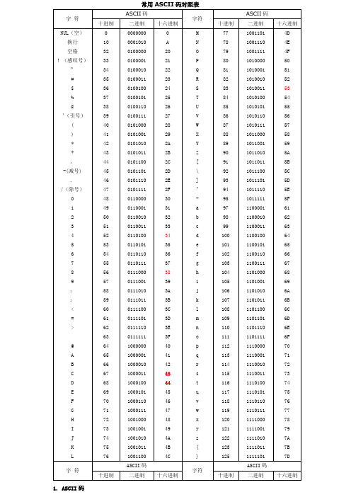
常用ASCII码对照表1. ASCII码在计算机内部,所有的信息最终都表示为一个二进制的字符串。
每一个二进制位(bit)有0和1两种状态,因此八个二进制位就可以组合出256种状态,这被称为一个字节(byte)。
也就是说,一个字节一共可以用来表示256种不同的状态,每一个状态对应一个符号,就是256个符号,从0000000到。
上个世纪60年代,美国制定了一套字符编码,对英语字符与二进制位之间的关系,做了统一规定。
这被称为ASCII码,一直沿用至今。
ASCII码一共规定了128个字符的编码,比如空格“SPACE”是32(十进制的32,用二进制表示就是00100000),大写的字母A是65(二进制01000001)。
这128个符号(包括32个不能打印出来的控制符号),只占用了一个字节的后面7位,最前面的1位统一规定为0。
2、非ASCII编码英语用128个符号编码就够了,但是用来表示其他语言,128个符号是不够的。
比如,在法语中,字母上方有注音符号,它就无法用ASCII码表示。
于是,一些欧洲国家就决定,利用字节中闲置的最高位编入新的符号。
比如,法语中的é的编码为130(二进制)。
这样一来,这些欧洲国家使用的编码体系,可以表示最多256个符号。
但是,这里又出现了新的问题。
不同的国家有不同的字母,因此,哪怕它们都使用256个符号的编码方式,代表的字母却不一样。
比如,130在法语编码中代表了é,在希伯来语编码中却代表了字母Gimel (),在俄语编码中又会代表另一个符号。
但是不管怎样,所有这些编码方式中,0—127表示的符号是一样的,不一样的只是128—255的这一段。
至于亚洲国家的文字,使用的符号就更多了,汉字就多达10万左右。
一个字节只能表示256种符号,肯定是不够的,就必须使用多个字节表达一个符号。
比如,简体中文常见的编码方式是GB2312,使用两个字节表示一个汉字,所以理论上最多可以表示256x256=65536个符号。
- 1、下载文档前请自行甄别文档内容的完整性,平台不提供额外的编辑、内容补充、找答案等附加服务。
- 2、"仅部分预览"的文档,不可在线预览部分如存在完整性等问题,可反馈申请退款(可完整预览的文档不适用该条件!)。
- 3、如文档侵犯您的权益,请联系客服反馈,我们会尽快为您处理(人工客服工作时间:9:00-18:30)。
Material behaviourBallistic and numerical simulation of impacting goods on conveyor belt rubberW.Molnar a,*,S.Nugent a,M.Lindroos b,M.Apostol b,M.Varga aa AC2T research GmbH,Viktor-Kaplan-Straße2C,2700Wiener Neustadt,Austriab Tampere Wear Center,Department of Materials Science,Tampere University of Technology,P.O.Box589,33101Tampere,Finlanda r t i c l e i n f oArticle history:Received27October2014 Accepted2December2014 Available online11December2014Keywords:RubberBallistic impactSimulationTribologyConveyor belt a b s t r a c tImpact loading is an important process in the transport industry as it causes wear and failure of critical components.Conveyor belts are of particular importance as they are used in practically every industry where large quantities of goods are moved over short(<10m) or long distances(>1km).To investigate stress levels inside the material during impact loading,a gas gun was utilized to shoot9mm spherical steel balls onto the surface of a rubber conveyor belt.A high speed video recording system was employed in order to determine penetration depth and dissipated energy of the steel ball.Maximal penetration depths of up to3.9mm and maximal dissipated energies of up to86.8%were measured. Additionally,a numerical simulation using smooth particle applied mechanics was con-ducted and compared to the experimental results obtained with the gas gun.The calcu-lated von Mises stresses affected the conveyor belts up to a maximum depth of8.8mm with at least20MPa.Maximum von Mises stresses were calculated to reach60MPa.©2014Elsevier Ltd.All rights reserved.1.IntroductionWear and failure of critical components are major con-cerns in every industry.Therefore,preventing or slowing down wear is one of the most important,but also most challenging,aspects of design.In this case,the loading process of rubber based conveyor belts is of particular in-terest.Depending on the application,conveyor belts can be loaded with hundreds of tons of goods every hour,which causes elastic,as well as plastic,deformation of the mate-rial and,over time,wear.The belt can make up to70%of the total costs of a transport system(calculated as cost per lifetime)[1],emphasising the importance of its wear resistance.To tackle this problem,one mustfirst understand the process of loading and impacting.One option is to run a large number of tests and experimentally simulate every possible outcome.Unfortunately,this is very time-consuming and expensive and,in most cases,impracti-cable.An elegant solution is a numerical simulation,which can quickly deliver values for set parameters once a suitable model has been chosen and corresponding code written. Such simulation can also give insight on phenomena that are not directly accessible via practical experiments,such as stress inside the material,change of contact geometry or tribo-chemical effects[2].Of course,there is still a need for experimentally acquired results to validate the chosen model.Over the years,different experimental setups have been designed to test materials for their impact related proper-ties,generating data that can be used to compare with data from numerical simulations.Wang et al.[3]used a high-speed crash system,where a trolley was accelerated by an elastic rope onto a rigid wall.A numerical simulation with a finite element model provided validation of data.Another possible setup includes a gas gun to simulate single particle impact,which was reported by Apostol et al.[4].Currently,*Corresponding author.E-mail address:molnar@ac2t.at(W.Molnar).Contents lists available at ScienceDirect Polymer Testingjou rn al homepage:/l ocate/polytest/10.1016/j.polymertesting.2014.12.0010142-9418/©2014Elsevier Ltd.All rights reserved.Polymer Testing42(2015)1e7impact simulations are used to predict impact-related wear due to erosion[5,6],blast resistance[7]and ballistics[8].In literature,numerical simulations,whether they are based on continuum,discrete or statistical methods,are often utilized in modelling tribological phenomena to enhance understanding of problems that are not accessible through experimental approaches alone[9].It is also possible to model such phenomena with a particle-based method:the smoothed particle applied mechanics (SPAM),as described recently by Sun et al.[10].This method relies on particles shifting around a defined grid according to equations of motion.The physical properties being investigated are gained through interpolation between these mass-carrying particles.Since the interpolation is a summation of the influence by neighbouring particles,theydo not carry volume elements,but parts of it,and summa-tion gives the quantity investigated.SPAM-related models have been used successfully in the past by Johnson et al.[11] to simulate pared to simulation methods like finite elements,SPAM can deal more efficiently with large deformations,which are expected when investigating rub-ber,and offer better accuracy in such situations.Depending on the kinetic energy of the impacting ball, wear and damage mechanisms can differ greatly.Thus,the model must be adjusted to the specific material pairing and kinetic energy.A visco-elastic model is needed in this case, as the objects being investigated are rubber conveyor belts.A couple of models have been used in literature to simulate visco-elastic impact[12].For modelling linear visco-elasticity,the well-established Kelvin-Voigt model and the Maxwell model can be used as a basis.This work will utilize the Kelvin-Voigt model,which includes a purely viscous dampener and a purely elastic spring.The SPAM model will contain a purely elastic material together with a viscous term,representing spring and dampener.Therefore,this work will focus on understanding the impact situation,with an emphasis on the stresses present during the loading process of rubber conveyor belts.In contrast to other works,which concentrate on homoge-nous materials to reduce the number of interpretable pa-rameters,this work tries to take the influence of the carcass into account,which more accurately reflects the practical usage of conveyor belts.2.Experimental2.1.MaterialsA basic schematic is shown in Fig.1,illustrating the complex makeup and material combination of a state of the art conveyor belt,which is composed of:A4mm thick rubber top layer and three layers of an interwoven polyester(warp)-polyamide(weft)carcass with skim layers (made of soft rubber)between them to improve the tensile strength of the belt.A2mm rubber bottom layer completes the conveyor belt and provides sufficient friction to the drive pulley during service.Two commercially available Styrene-Butadien-Rubber (SBR)based conveyor belts,Semperit Multiply D(Sample A)and Transconti NQ(Sample B),were chosen for these experiments.Additionally,Semperit N17was selected (Sample C).This particular belt is also SBR based and fea-tures additionally a deformingfleece for better processing. Shore A hardness was measured for all three samples and revealed values of65,63and71for Samples A,B,and C, respectively.Square plates,with lateral dimensions of180Â180mm and a total thickness of10mm,were sawn from of the original conveyor belts.These samples were thenfixed to a tiltable table using steel clamps.2.2.Impact testingThe impact tests at high velocity were performed using a High Velocity Particle Impactor(HVPI).A schematic drawing of the device is presented in Fig.2.The HVPI consists of a smooth bore barrel connected to a pressurised air tank so that9mm balls of various materials can be launched onto prepared samples.To monitor the velocity at impact,a speed measurement device was placed just before the target assembly.The target assembly is angled at 45 and consists of the samplesfixed onto a steel support with clamps.The impact was monitored by a high speed camera and evaluated for subsequent analysis.The HVPI device uses pressurized air to launch spherical projectiles in a controlled manner against a piece of conveyor belt placed at1m distance from the end of the barrel.A stainless steel ball of9mm in diameter and2.98g in weight was used as a projectile.The projectile balls were fired against the samples at a constant velocity of37m/s, which corresponds to a kinetic energy prior the impact of 2.04J.The incident velocity of the projectile was measured by a commercial timing device placed in front of the target assembly.The impact tests were performed at an angle of 45 with a precision of±1 .Each sample was impacted ten times to observe effects of hysteresis or damage caused by previous impacts and to ensure statistical significance.The fractions of dissipated energy of the initial kinetic energies,maximum penetration depths and reflected an-gles were determined by analysing several overlapping high speed images.Fig.3illustrates the overlapping tech-nique,where the yellow dash-dot line defines the impact surface(zero line)and the blue circles highlight the surface of the impacting steel ball.To calculate the exit velocity,the distance travelled(D s) between frames after the impact event was calculated by tracking a specific point,such as the centroid of theball.Fig.1.Schematic cross-section of a state of the art conveyor belt.W.Molnar et al./Polymer Testing42(2015)1e7 2The exit velocity is then used to calculate the dissipated energy (E d )fractions.E d ¼m p Àv 2i Àv 2eÁ2;(1)where m p ,v i ,v e ,represent the mass of the particle,themeasured incident velocity and the calculated exit velocity of the particle,respectively.The maximum penetration depths (D p )were also quanti fied via image analysis by determining the maximum de flection of the rubber surface with respect to the original surface (zero line)during the impact event.In addition,the projectile velocity and deceleration were calculated as functions of time by using all captured high speed images in order to analyze changes in material properties throughout the experiment.2.3.Simulation e SPAMThe simulations were done with the scheme of Smoothed Particle Applied Mechanics close to theformulation of Nugent et al.[14].Any continuum or field function f(r,v)at a location r with a velocity v is represented as a weighted sum of the contributions from the neigh-bouring particles [15]:〈f ðr ;v Þ〉¼mX N j ¼11r ðr j Þf ðr j ;v j Þw ðj r Àr j j ;h Þ(2)So,N particles each carry the same mass m and con-tinuum values,such as density r j .If one applies the gradient to this function,it only applies to r ,so only the gradient of the kernel has to be considered.The kernel.w ij ¼w ðj r i Àr j j ;h Þ(3)is usually an even function with a finite carrier of radius h ,called the smoothing length.We use the Lucy kernel in this work [14,16],which vanishes smoothly at radius r !h .For simulation of solids,the equations have to be modi fied regarding the representation of the stress-strain relation s -ε[17].With the density being integrated from the continuity relation,the SPAM equations of motion (equations (4)e (8))become:d r ðr i Þ¼m X N j ¼1ðv i Àv j ÞV i w ij(4)dr idt¼v i (5)d v i dt ¼m X N j ¼1s i i þs ij !$V i w ij þF v þF e(6)d εi dt¼Àm 2X Nj ¼11ffiffiffiffir i p r j ÀÀv i Àv j Á5V w ij þð…Þt Á(7)d s i dt ¼l tr d εi dtþ2m d εidt(8)For the force due to viscosity F v ,we use the arti ficial viscosity described by Monaghan [15],with a beingaFig.2.Schematic of the high velocity particle impactor (HVPI)[13].Fig.3.Five stages of the impact event recorded with a high speed cameraduring HVPI testing,showing the analysed values [13].W.Molnar et al./Polymer Testing 42(2015)1e 73viscous parameter and h ¼a r hc/20being the viscosity,where c is the velocity of sound.F e represents external forces,for instance boundary forces.Boundary conditions are modelled by mirror particles [18],ideal plasticity by multiplying the stress with a reduction factor,which compares the yield with the von Mises stress [17],and tangential plasticity with a tangential adjustment of the yield.The whole simulated area equals an isotropic plate with dimensions of 28Â28Â10mm (LxWxH)with an incompressible layer placed on the bottom (the opposite side from the impact).3.Results3.1.Experimental impact simulationThe penetration depth and dissipated energy acquired during the experiments with the HVPI gas gun can be observed in Fig.4.As expected,the majority of the steel ball's kinetic energy was dissipated by the impact on the conveyor belt surface (Fig.4a,b).From the original kinetic energy of 2J,the ball lost between 86.1%(Sample A)and 86.8%(Samples B and C).All three samples show practically the same amount of dissi-pated energy (which is why only a very narrow range is shown in Fig.4b)and also feature very similar evolution of dissipated energy during impact.It can,therefore,be concluded that the dissipated energy shows no relation to Shore A hardness,which is different for the samples.The penetration depths (Fig.4c,d)reached a maximum of 3.9mm for Sample A,3.6mm for Sample B and 3.1mm for Sample C.It is also not surprising that the deforming fleece in Sample C causes the lowest penetration depth,as the textile fibres distribute the force of the impact more ef ficiently and stiffen the rubber because of the fibres'higher elastic modulus.It is widely accepted that there are no universal equa-tions for calculating a rubber's visco-elastic properties from its mechanical properties,and mathematical models only apply for a very limited set of parameters [19].Further-more,at such high penetration depths,the carcass and skim layers are starting to interact with the impacting steel ball.Hence,it is not surprising that the penetration depths do not correlate with the Shore A hardness of the rubber covers,which is used more for its historical importance than its applicability [20].Another interesting detail is that the dissipation of the energy takes roughly 0.25ms,while it takes 0.45ms for the penetration depth to revert to 0mm.It seems that the energy is only dissipated in considerable amounts when certain penetration depths are reached.The steel ball loses most of its speed in an interval of 0.15ms,so only within three data-points.It can be concluded that the recording speed of 20.000fps (one frame every 0.05ms)was probably too low to investigate certain details of the impact.However,the image quality (reduced resolution)deteriorated at higher recording speeds and reduced the accuracy of the optical analysis.Ten impacts were performed per sample and used to calculate the standard deviations in Figs.4b,d.RubbermayFig.4.Dissipated energy during HVPI testing as functions of time (a)and as maximum values (b)for Samples A,B and C.Analogously,penetration depths functions of time (c)and maximum penetration depths (d)for the three samples are shown.W.Molnar et al./Polymer Testing 42(2015)1e 74show a hysteresis depending on its loading process history [19],but no signs of hysteresis were observed at HVPI testing.Also,no signs of wear were observed in the impact zone after the investigation.The standard deviations overlap for the maximum dissipated energy,therefore their absolute values can be considered equal,although the maximum penetration depths show clear differences.Consequently,the results from Fig.4show very similar results for all three samples regarding dissipated energy.Samples A and B are again similar,as their standard de-viations overlap.Sample C,on the other hand,clearly exhibits a lower value than the other two.This is probably due to the deforming fleece worked into the top layer of Sample C.3.2.Numerical impact simulationAll of the experimentally acquired values were used as a foundation for a numerical simulation using SPAM.Fig.5shows the results of the SPAM simulation as described above.As exact values are unknonwn,the simulations were conducted in the form of a parameter variation study,where the E-modulus and the viscosity parameter a were varied to determine the curves closest to the experimental values.Calculations were made for E-moduli of 0.01,0.05and 0.1GPa,as rubber can be expected to exhibit values in this region.Also,values of 0.3,0.5and 0.7were taken for the viscosity parameter a ,which is the standard range for elastomers.An E-modulus of 0.01GPa and a ¼0.3in the SPAM simulation produced yield results that best fit the experi-mental curves and,therefore,best describe the behaviourof the investigated rubber conveyor belts.The penetration depth (Fig.5a)reached maximum values of 3mm,which is in good agreement with the experimental values varying from 3.1mm to 3.4mm.The calculated time for the dura-tion of impact,on the other hand,does not fit the experi-mental values so well:0.45and 0.50ms were measured during the experiments,while calculated values reach 0.7ms.The evolution of the ball's dissipated energy (Fig.5b)most closely replicates the experimental results when E is set to 0.10GPa and a is set to 0.5.As before,a large differ-ence can be seen between the duration of the impact calculated numerically (0.2ms)and measured experi-mentally (0.45ms).A minimum was observed in the function of the ball's energy over time,which corresponds to the point where the steel ball had its lowest velocity.Then,the energy rises slightly,as the stored energy in the rubber is partly retransferred to the steel ball.This effect was not observable in the experiments,as the recording speed was too low to investigate such details.Clearly,the numerical simulation offers improved insight into impact behaviour.Fig.6shows the distribution of the von Mises stresses and a 3D illustration of the rubber material during different stages of the impact calculated with the SPAM simulation.The simulation of the von Mises stresses revealed that the highest concentration of stress can be expected along the impact direction of the steel ball and reaches values up to 60MPa.Although the rubber is affected by stress practically over the entire thickness during the impact,the impact region near the trailing edge is affected muchless.Fig.5.Penetration depth (a)and dissipated energy of the ball (b)calculated by adjusting the E-modulus (E)and the viscosity parameter (a )in SPAM simulations.W.Molnar et al./Polymer Testing 42(2015)1e 754.DiscussionContrary to the simulation with a sliding ball on rubber conducted by Fukahori et al.[21],there was no second high stress concentration at the trailing edge.This shows that these two kinds of motion cannot be compared directly,as the stress distribution takes a different form.Consequently,impact on rubber cannot be investigated correctly by sliding experiments or simulations.Other,more impact-related,works in literature concentrate on military appli-cations,such as the propagation of shockwaves and dam-age caused by bullets (Leavy et al.[8]),involving too much kinetic energy to be considered realistic for impacts on conveyor belt transport systems.Further interesting in-vestigations were conducted by Cenna et al.[22],who used a similar gas gun to study the impact on ductile materials.Due to the ductility,the deformation remained intact,allowing greater insight into the development of the deformation and how the material was affected.Cenna et al.also observed two zones.The first zone,situated in the impact direction of a spherical particle,featured high stress and deformation.The second zone represented the defor-mation of the bulk and was shaped more symmetrically around the impact.The numerical simulation conducted in this work con firmed the observations made by Cenna et al.,as the same stress distribution was calculated.Fig.7shows the affected depth,which is de fined here as the depth of the sample affected by stresses of 20MPa or more,and the depth where the highest stress concentra-tion was found (depth of highest stress).The dotted line illustrates the thickness of the top layer,i .e .the part of the rubber that is intended to absorb the impact.The values were calculated from the simulation depicted in Fig.6.At 0.07ms,the early state of impact with only 1.6mm penetration depth,the affected depth already reaches 4.7mm and in fluences the carcass.At its maximum,the affected depth reaches a value of 8.8mm e far beyond the thickness of the 4mm top layer and,theoretically,already reaching into the bottom layer beyond the carcass.The depths of highest stress,on the other hand,do not exceed 4mm and remain concentrated slightly above the carcass.Therefore,the carcass already crucially in fluences the impact behaviour of rubber conveyor belts at relatively low energy levels.As the calculations were conducted without taking a carcass into consideration,the simulated impact behaviour does not match with that observed during ex-periments perfectly.Nonetheless,useful insight into sur-face wear and destruction-related phenomena was gained by this investigation:Affected depths already exceed the top layer thickness by far at 2.04J impact.For high-impact environments,thick top layers should be considered in order to guarantee long life cycles of conveyor belts.The next step for understanding the complex conveyor belt structure and tailoring wear resistant solutions should involve consideration of the carcass as well,despite its complex model,dif ficult reproduction and increased de-mand in computing capability.5.ConclusionsThe results from the ballistic experiments with a gas gun served as a basis for the SPAM-based numerical simulation.The kinetic energy of the steel ball and the penetration depth was recorded throughout the test and then compared to the simulated values.While fitting the kinetic energies and penetration depths was done satis-factorily,the calculated time until impact was always about 25%shorter than in the experiments.Also,different pa-rameters for E and a were necessary to ensure the best fit for each quantity.Therefore,it can be deduced that the chosen model lacks some details.It would be necessary to apply a more complex model that takes into account the in fluence and behaviour of the carcass and skim layers,as the penetration depths are high enough to make consid-ering the in fluence of these parts necessary.Nonetheless,the stress distribution was calculated satisfactorily.The maximum affected depth during the impacts reaches 8.8mm,proving that not only the top layer is affected,but also the carcass.Hence,thick top layers are worth consid-ering for application,depending on kinetic energy and size of the impacting particles.AcknowledgmentsThis work was funded by the “Austrian Comet-Pro-gram ”(governmental funding program forpre-competitiveFig.6.Von Mises stress distribution and 3D illustration of the rubber ma-terial during different stages of the impact with parameter:E ¼0.01GPa and a ¼0.3.Fig.7.Affected stress and the depth of the highest stress concentration calculated from the numerical simulation.Parameters:E ¼0.01GPa;a ¼0.3.W.Molnar et al./Polymer Testing 42(2015)1e 76research;Project XTribology,no.824187)via the Austrian Research Promotion Agency(FFG)and was carried out at the“Austrian Center of Competence for Tribology”(AC2T research GmbH)and at Tampere Wear Center,Department of Materials Science,Tampere University of Technology. The authors thank Marcela Petrica for the research idea and for enabling this work.References[1]R.Hartlieb,v.Wallthor,Beitr€a ge zu einer betriebssicherenGestaltung von Gurtf€o rderanlagen im Steinkohlebergbau unter Tage,Berg-und Hüttenm€a nnische Monatshefte120(8)(1975) 371e380.[2]M.Renouf,F.Massi,N.Fillot,A.Saulot,Numerical tribology of a drycontact,Tribology International44(2011)834e844.[3]Z.Wang,H.Tian,Z.Lu,W.Zhou,High-speed axial impact ofaluminium honeycomb e Experiments and simulations,Compos-ites:Part B56(2014)1e8.[4] E.Sarlin,M.Apostol,M.Lindroos,V.-T.Kuokkala,J.Vuorinen,T.Lepist€o,M.Vippola,Impact properties of novel corrosion resistant hybrid structures,Composite Structures108(2014)886e893. [5]H.Ashrafizadeh, F.Ashrafizadeh,A numerical3D simulation forprediction of wear caused by solid particle impact,Wear276e277 (2012)75e84.[6]M.Varga,Ch.Goniva,K.Adam,E.Badisch,Combined experimentaland numerical approach for wear prediction in feed pipes,Tribology International65(2013)200e206.[7]V.A.Phadnis,P.Kumar,A.Shukla,A.Roy,V.V.Silberschmidt,Opti-mising curvature of carbonfibre-reinforced polymer composite panel for improved blast resistance:finite-element analysis,Mate-rials and Design57(2014)719e727.[8]R.B.Leavy,J.D.Clayton,O.E.Strack,R.M.Brannon,E.Strassburger,Edge on impact simulations and experiments,Procedia Engineering 58(2013)445e452.[9]Editorial,Numerical Simulation Methods in Tribology:possibilitiesand limitations,Tribology International40(2007)915.[10]X.Sun,M.Sakai,Y.Yamada,Three-dimensional simulation of asolid e liquidflow by the DEM e SPH method,Journal of Computa-tional Physics248(2013)147e176.[11]G.R.Johnson,S.R.Beissel,Normalized smoothing functions for SPHimpact computations,International Journal of numerical methods in Engineering39(1993)2725e2741.[12]I.I.Argatov,Mathematical modeling of linear viscoelastic impact:application to drop impact testing of articular cartilage,Tribology International63(2013)213e225.[13]M.Apostol,V.-T.Kuokkala,ukkanen,R.Waudby,K.Holmberg,M.Lindroos.High velocity particle impactor e modeling and experimental verification of impact wear tests.WTC2013,5th World Tribology Congress8.-13.9.2013,Torino,Italy.[14]S.Nugent,H.A.Posch,Liquid drops and surface tension withsmoothed particle applied mechanics,Physical Review E62(2000) 4968e4975.[15]J.J.Monaghan,Smoothed particle hydrodynamics,Reports onProgress in Physics68(2005)1703e1759.[16]L.B.Lucy,A numerical approach to the testing of thefission hy-pothesis,The Astronomical Journal82(1977)1013e1024.[17]M.D.Fuller,The Application of Smooth Particle Hydrodynamics tothe Modelling of Solid Materials,PhD thesis,University of Leicester, 2010.[18]W.G.Hoover,in:Smoothed Particle Applied Mechanics,AdvancedSeries in Nonlinear Dynamics,vol.25,World Scientific,2006. [19]N.M.Vriend,A.P.Kren,Determination of the viscoelastic propertiesof elastomeric materials by the dynamic indentation method, Polymer Testing23(2004)369e375.[20] A.C.Bassi,F.Casa,Shore A hardness and thickness,Polymer Testing7(1987)165e175.[21]Y.Fukahori,P.Gabriel,J.J.C.Busfield,How does rubber truly slidebetween Schallamach waves and stick e slip motion?Wear266 (2009)288e296.[22] A.A.Cenna,N.W.Page,E.Kisi,M.G.Jones,Single particle impact testsusing gas gun and analysis of high strain-rate impact events in ductile materials,Wear271(2011)1497e1503.W.Molnar et al./Polymer Testing42(2015)1e77。