Eviews操作指导chapter14
Eviews操作手册
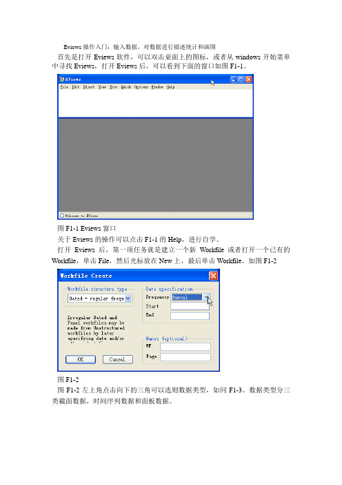
Eviews操作入门:输入数据,对数据进行描述统计和画图首先是打开Eviews软件,可以双击桌面上的图标,或者从windows开始菜单中寻找Eviews,打开Eviews后,可以看到下面的窗口如图F1-1。
图F1-1 Eviews窗口关于Eviews的操作可以点击F1-1的Help,进行自学。
打开Eviews后,第一项任务就是建立一个新Workfile或者打开一个已有的Workfile,单击File,然后光标放在New上,最后单击Workfile。
如图F1-2图F1-2图F1-2左上角点击向下的三角可以选则数据类型,如同F1-3。
数据类型分三类截面数据,时间序列数据和面板数据。
图F1-3图F1-2右上角可以选中时间序列数据的频率,见图F1-4。
图F1-4对话框中选择数据的频率:年、半年、季度、月度、周、天(5天一周或7天1周)或日内数据(用integer data)来表示。
对时间序列数据选择一个频率,填写开始日期和结束日期,日期格式:年:1997季度:1997:1月度:1997:01周和日:8:10:1997表示1997年8月10号,美式表达日期法。
8:10:1997表示1997年10月8号,欧式表达日期法。
如何选择欧式和美式日期格式呢?从Eviews窗口点击Options再点击dates and Frequency conversion,得到窗口F1-5。
F1-5的右上角可以选择日期格式。
图F1-5假设建立一个月度数据的workfile,填写完后点OK,一个新Workfile就建好了。
见图F1-6。
保存该workfile,单击Eviews窗口的save命令,选择保存位置即可。
图F1-6新建立的workfile之后,第二件事就是输入数据。
数据输入有多种方法。
1)直接输入数据,见F1-7在Eviews窗口下,单击Quick,再单击Empty group(edit series),直接输数值即可。
注意在该窗口中命令行有一个Edit+/-,可以点一下Edit+/-就可以变成如图所示的空白格,输完数据后,为了避免不小心改变数据,可以再点一下Edit+/-,这时数据就不能被修改了。
eviews使用指南与案例

eviews使用指南与案例Eviews使用指南与案例。
Eviews是一款广泛用于经济学、金融学和统计学等领域的专业数据分析软件,其强大的数据处理和分析功能受到了广大用户的青睐。
本文将为大家介绍Eviews的基本使用方法,并结合实际案例进行详细说明,希望能够帮助大家更好地掌握这一工具。
首先,我们来看一下Eviews的基本操作流程。
在打开Eviews软件后,首先需要新建一个工作文件,选择“File”中的“New”选项,然后选择“Workfile”来创建一个新的数据工作文件。
在新建工作文件后,可以导入需要分析的数据,Eviews支持导入多种格式的数据文件,如Excel、CSV等,用户可以根据实际情况选择合适的数据导入方式。
在导入数据后,我们可以进行数据的预处理工作,包括数据的清洗、变量的转换、缺失值的处理等。
Eviews提供了丰富的数据处理工具,用户可以根据需要进行相应的操作。
接下来,我们可以进行数据的描述性统计分析,包括数据的均值、标准差、相关系数等指标的计算,以及绘制数据的直方图、散点图等图表来直观地展现数据的特征。
在数据的基本分析完成后,我们可以进行更深入的统计分析,如回归分析、时间序列分析等。
Eviews提供了丰富的统计分析工具,用户可以根据实际需求选择合适的方法进行分析。
在进行统计分析时,我们还可以进行模型的建立和检验,以及参数的估计和显著性检验等工作,从而得到对实际问题的有效解释和预测。
除了基本的数据分析功能外,Eviews还提供了强大的数据可视化工具,用户可以通过图表、表格等形式将分析结果直观地展现出来。
同时,Eviews还支持数据的导出和报告的生成,用户可以将分析结果导出到Word、Excel等格式的文件中,或者直接在Eviews中生成报告,方便进行结果的分享和展示。
在实际应用中,Eviews可以广泛用于经济预测、金融风险分析、市场调研等领域,其强大的数据分析功能可以帮助用户更好地理解和解决实际问题。
Eviews操作完整操作指引

1.EVIEWS基础 (4)1.1. E VIEWS简介 (4)1.2. E VIEWS的启动、主界面和退出 (4)1.3. E VIEWS的操作方式 (8)1.4. E VIEWS应用入门 (9)1.5. E VIEWS常用的数据操作 (21)2.一元线性回归模型 (32)2.1. 用普通最小二乘估计法建立一元线性回归模型 (32)2.2. 模型的预测 (39)2.3. 结构稳定性的C HOW检验 (43)3. 多元线性回归 (49)3.1. 用OLS建立多元线性回归模型 (49)3.2. 函数形式误设的RESET检验 (56)4. 非线性回归 (59)4.1. 用直接代换法对含有幂函数的非线性模型的估计 (59)4.2. 用间接代换法对含有对数函数的非线性模型的估计 (61)4.3. 用间接代换法对CD函数的非线性模型的估计 (64)4.4. NLS对可线性化的非线性模型的估计 (66)4.5. NLS对不可线性化的非线性模型的估计 (70)4.6. 二元选择模型 (75)5. 异方差 (83)5.1. 异方差的戈得菲尔德——匡特检验 (83)5.2. 异方差的WHITE检验 (87)5.3. 异方差的处理 (91)6. 自相关 (95)6.1. 自相关的判别 (95)6.2. 自相关的修正 (101)7. 多重共线性 (105)7.1. 多重共线性的检验 (105)7.2. 多重共线性的处理 (112)8. 虚拟变量 (115)8.1. 虚拟自变量的应用 (115)8.2. 虚拟变量的交互作用 (121)8.3. 二值因变量:线性概率模型 (123)9. 滞后变量模型 (129)9.1. 自回归分布滞后模型的估计 (129)9.2. 多项式分布滞后模型的参数估计 (136)10. 联立方程模型 (142)10.1. 联立方程模型的单方程估计方法 (142)10.2. 联立方程模型的系统估计方法 (148)2。
Eviews操作教程_完整版

Eviews操作教程_完整版1.EVIEWS基础 (3)1.1. E VIEWS简介 (3)1.2. E VIEWS的启动、主界⾯和退出 (3)1.3. E VIEWS的操作⽅式 (6)1.4. E VIEWS应⽤⼊门 (6)1.5. E VIEWS常⽤的数据操作 (15)2.⼀元线性回归模型 (24)2.1. ⽤普通最⼩⼆乘估计法建⽴⼀元线性回归模型 (24) 2.2. 模型的预测 (30)2.3. 结构稳定性的C HOW检验 (34)3. 多元线性回归 (39)3.1. ⽤OLS建⽴多元线性回归模型 (39)3.2. 函数形式误设的RESET检验 (45)4. ⾮线性回归 (48)4.1. ⽤直接代换法对含有幂函数的⾮线性模型的估计 (48) 4.2. ⽤间接代换法对含有对数函数的⾮线性模型的估计 (50) 4.3. ⽤间接代换法对CD函数的⾮线性模型的估计 (53)4.4. NLS对可线性化的⾮线性模型的估计 (55)4.5. NLS对不可线性化的⾮线性模型的估计 (58)4.6. ⼆元选择模型 (62)5. 异⽅差 (68)5.1. 异⽅差的⼽得菲尔德——匡特检验 (68)5.2. 异⽅差的WHITE检验 (72)5.3. 异⽅差的处理 (75)6. ⾃相关 (79)6.1. ⾃相关的判别 (79)6.2. ⾃相关的修正 (83)7. 多重共线性 (87)7.1. 多重共线性的检验 (87)7.2. 多重共线性的处理 (92)8. 虚拟变量 (94)8.1. 虚拟⾃变量的应⽤ (94)8.2. 虚拟变量的交互作⽤ (99)8.3. ⼆值因变量:线性概率模型 (101)9. 滞后变量模型 (106)9.1. ⾃回归分布滞后模型的估计 (106)9.2. 多项式分布滞后模型的参数估计 (111)10. 联⽴⽅程模型 (116)10.1. 联⽴⽅程模型的单⽅程估计⽅法 (116)10.2. 联⽴⽅程模型的系统估计⽅法 (120)2..1.Eviews基础1.1.Eviews简介Eviews:Econometric Views(经济计量视图),是美国QMS公司(Quantitative Micro Software Co.,⽹址为/doc/8e38170bbed126fff705cc1755270722192e59b1.html )开发的运⾏于Windows环境下的经济计量分析软件。
超详细的eviews操作手册

EViews 操作手册目录第一章序论第二章EViews 简介第三章EViews 基础第四章基本数据处理第五章数据操作第六章EViews 数据库第七章序列第八章组第九章应用于序列和组的统计图第十章图、表和文本对象第十一章基本回归模型第十二章其他回归方法第十三章时间序列回归第十四章方程预测第十五章定义和诊断检验第十六章ARCH和GARCH估计第十七章离散和受限因变量模型第十八章对数极大似然估计第十九章系统估计第二十章向量自回归和误差修正模型第一章绪论EViews 为我们提供了基于WINDOWS平台的复杂的数据分析、回归及预测工具,通过EViews能够快速从数据中得到统计关系,并根据这些统计关系进行预测。
EViews在系统数据分析和评价、金融分析、宏观经济预测、模拟、销售预测及成本分析等领域中有着广泛的应用。
操作手册共分五部分:第一部分:EViews 基础介绍EViews 的基本用法。
另外对基本的Windows 操作系统进行讨论,解释如何使用EViews来管理数据。
第二部分:基本的数据分析描述使用EViews 来完成数据的基本分析及利用EViews 画图和造表来描述数据。
第三部分:基本的单方程分析讨论标准回归分析:普通最小二乘法、加权最小二乘法、二阶最小二乘法、非线性最小二乘法、时间序列分析、方程检验及预测。
第四部分:扩展的单方程分析介绍自回归条件异方差(ARCH)模型、离散和受限因变量模型、和对数极大似然估计。
第五部分:多方程分析描述利用方程组来估计和预测、向量自回归、误差修正模型、状态空间模型、截面数据/ 时间序列数据、及模型求解。
第二章EViews 简介§2.1 什么是EViewsEViews 是在大型计算机的TSP (Time Series Processor)软件包基础上发展起来的新版本,是一组处理时间序列数据的有效工具。
1981年QMS (Quantitative Micro Software) 公司在Micro TSP基础上直接开发成功EViews 并投入使用。
eviews操作说明解析

删除( Delete ):在当前(激活)窗口中删除对象。若 当前(激活)窗口是工作文件窗口,则删除已选定的对 象。 复制对象(Copy Object):复制一个
• 打印(Print):打印当前(激活)窗口中的内容。
功能选择(View Options):改变当前对象的操作功能。 随着当前对象性质的不同,功能选择(View Options) 中的内容也不同。
•撤销(Undo):撤销最后一次操作,恢复到最后一次操
作以前的状态。
• 剪切(Cut):删除用拖动覆盖法选定的内容并放入剪切
板。
•复制(Copy):把所选定的内容存入剪切板。 •粘贴(Paste):把复制的内容粘贴到光标所在的位置。
•清除(Delete):清除所选定的内容。 •进行(Next):执行下一个预指定操作。 •合并(Merge):把一个文件合并到一个待修改
二、主菜单说明
(1) File键: 主菜单中File键的主要功能 :
•新建(New):创建新工作文件( New Workfile)。 •打开(Open):打开已有的工作文件。 •保存(Save):使用现存的文件名保存当前的工作文件,如
果文件尚未命名,则要求给出文件名,并指出保存路Байду номын сангаас。
•另存(Save as):用另一个文件名保存当前文件。 •关闭(Close):关闭当前的窗口。如尚未做最后保
存,将出现对话框提醒你保存。
•打印(Print):打印当前(激活)窗口的显示结果。
•打印设置(Print
Setup): 通过打印设置选择对话 框控制打印设置。
•运行(Run):运行EViews程序文件。 •退出(Exit):关闭所有窗口,并退出EViews。
Eviews使用教程

计量经济学软件包Eviews 使用说明一、启动软件包假定用户有Windows95/98的操作经验,我们通过一个实际问题的处理过程,使用户对EViews 的应用有一些感性认识,达到速成的目的。
1、Eviews 的启动步骤:进入Windows /双击Eviews 快捷方式,进入EViews 窗口;或点击开始 /程序/Econometric Views/ Eviews ,进入EViews 窗口。
2、EViews 窗口介绍标题栏:窗口的顶部是标题栏,标题栏的右端有三个按钮:最小化、最大化(或复原)和关闭,点击这三个按钮可以控制窗口的大小或关闭窗口。
菜单栏:标题栏下是主菜单栏。
主菜单栏上共有7个选项: File ,Edit ,Objects ,View ,Procs ,Quick ,Options ,Window ,Help 。
用鼠标点击可打开下拉式菜单(或再下一级菜单,如果有的话),点击某个选项电脑就执行对应的操作响应(File ,Edit 的编辑功能与Word, Excel 中的相应功能相似)。
命令窗口:主菜单栏下是命令窗口,窗口最左端一竖线是提示符,允许用户在提示符后通过键盘输入EViews (TSP 风格)命令。
如果熟悉MacroTSP (DOS )版的命令可以直接在此键入,如同DOS 版一样地使用EViews 。
按F1键(或移动箭头),键入的历史命令将重新显示出来,供用户选用。
命令窗口信息栏路径主显示窗口(图一)主显示窗口:命令窗口之下是Eviews的主显示窗口,以后操作产生的窗口(称为子窗口)均在此范围之内,不能移出主窗口之外。
状态栏:主窗口之下是状态栏,左端显示信息,中部显示当前路径,右下端显示当前状态,例如有无工作文件等。
Eviews有四种工作方式:(1)鼠标图形导向方式;(2)简单命令方式;(3)命令参数方式[(1)与(2)相结合)] ;(4)程序(采用EViews命令编制程序)运行方式。
Eviews操作教程-完整版汇总
1.EVIEWS基础 (3)1.1. E VIEWS简介 (3)1.2. E VIEWS的启动、主界面和退出 (3)1.3. E VIEWS的操作方式 (5)1.4. E VIEWS应用入门 (6)1.5. E VIEWS常用的数据操作 (15)2.一元线性回归模型 (24)2.1. 用普通最小二乘估计法建立一元线性回归模型 (24)2.2. 模型的预测 (30)2.3. 结构稳定性的C HOW检验 (34)3. 多元线性回归 (39)3.1. 用OLS建立多元线性回归模型 (39)3.2. 函数形式误设的RESET检验 (45)4. 非线性回归 (48)4.1. 用直接代换法对含有幂函数的非线性模型的估计 (48)4.2. 用间接代换法对含有对数函数的非线性模型的估计 (50)4.3. 用间接代换法对CD函数的非线性模型的估计 (53)4.4. NLS对可线性化的非线性模型的估计 (55)4.5. NLS对不可线性化的非线性模型的估计 (58)4.6. 二元选择模型 (62)5. 异方差 (68)5.1. 异方差的戈得菲尔德——匡特检验 (68)5.2. 异方差的WHITE检验 (72)5.3. 异方差的处理 (75)6. 自相关 (79)6.1. 自相关的判别 (79)6.2. 自相关的修正 (83)7. 多重共线性 (87)7.1. 多重共线性的检验 (87)7.2. 多重共线性的处理 (92)8. 虚拟变量 (94)8.1. 虚拟自变量的应用 (94)8.2. 虚拟变量的交互作用 (99)8.3. 二值因变量:线性概率模型 (101)9. 滞后变量模型 (105)9.1. 自回归分布滞后模型的估计 (105)9.2. 多项式分布滞后模型的参数估计 (110)10. 联立方程模型 (115)10.1. 联立方程模型的单方程估计方法 (115)10.2. 联立方程模型的系统估计方法 (119)21.Eviews基础1.1. Eviews简介Eviews:Econometric Views(经济计量视图),是美国QMS公司(Quantitative Micro Software Co.,网址为)开发的运行于Windows环境下的经济计量分析软件。
- 1、下载文档前请自行甄别文档内容的完整性,平台不提供额外的编辑、内容补充、找答案等附加服务。
- 2、"仅部分预览"的文档,不可在线预览部分如存在完整性等问题,可反馈申请退款(可完整预览的文档不适用该条件!)。
- 3、如文档侵犯您的权益,请联系客服反馈,我们会尽快为您处理(人工客服工作时间:9:00-18:30)。
Chapter 14: Simultaneous Equations1.2.3.4. UE, 14.3.1)5.6.7.The naïve Keynesian macroeconomic model of the U.S. economy identified in UE, p. 477 will be used to demonstrate the two stage-least squares procedure. The data for this model is found in the EViews workfile named macro14.wf1 and it is printed in UE, Table 14.1, p. 478. Twovariables that are included in the macroeconomic model must be generated from other data series (see note at the bottom of UE, Table 14.1, p. 478).Generating time series for taxes and net exports using structural equations (UE, p. 477): Follow these steps to generate time series values for T (taxes) and NX (net exports) using the structural equations in the model:Step 1. Open the EViews workfile named Macro14.wf1.Step 2. To generate a new series named T for taxes, select Genr on the workfile menu bar, type T=Y-YD in the Enter equation: window, and click OK. A new series icon for T is created in theworkfile window.Step 3. To generate a new series named NX for net exports, select Genr on the workfile menu bar, type NX=Y-CO-I-G in the Enter equation: window, and click OK. A new series icon for NX is created in the workfile window.Step 4. Select Save on the workfile menu bar to save your changes.Estimating CO with least squares (UE, Equation 14.31, p. 481):Step 1. Open the EViews workfile named Macro14.wf1.Step 2. Select Objects/NewObject/Equation on the workfilemenu bar, enter CO C YD CO(-1)in the Equation Specification:window, and click OK to revealthe regression output to the right.Step 3. Select Name on the equationwindow menu bar, enter OLS_COin the Name to identify object:window, and click OK.Step 4. Select Save on the workfilemenu bar to save your changes.Estimating two-stage least squares regression using EViews TSLS method (UE, 14.3.1): To estimate the two-stage least squaresmodel printed in UE, Equation 14.29,follow these steps:Step 1. Open the EViews workfile namedMacro14.wf1.Step 2. Select Objects/NewObject/Equation on the workfilemenu bar, and select TSLS – Two-StageLeast Squares (TSNLS and ARMA) inthe Method: window under EstimationSettings: and the dialog will change toinclude an Instrument list: window (seegraphic on the right).Step 3. Enter CO C YD CO(-1) in theEquation Specification: window and C G T NX CO(-1) R(-1) in the Instrument list: window.1 The graphic above shows the relevant selections/entries highlighted in yellow. Click OK to reveal the Estimation Output view printed below. The yellow highlighted portions of theregression output reflect the selections made in the dialog window shown above.2Dependent Variable: COMethod: Two-Stage Least SquaresDate: 07/10/00 Time: 15:12Sample(adjusted): 1964 1994Included observations: 31 after adjusting endpointsInstrument list: C G T NX CO(-1) R(-1)t-StatisticErrorProb.Std.Variable CoefficientC -24.73014 34.90233 -0.708553 0.4845YD 0.441638 0.153839 2.870773 0.0077CO(-1) 0.540309 0.163000 3.314782 0.0025R-squared 0.997890 Mean dependent var 2445.210Adjusted R-squared 0.997739 S.D. dependent var 642.2594S.E. of regression 30.53734 Sum squared resid 26110.82F-statistic 6615.725 Durbin-Watson stat 0.982576Prob(F-statistic) 0.000000Step 4. Select Name on the equation window menu bar, enter TSLS_CO in the Name to identify object: window, and click OK.Step 5. Select Save on the workfile menu bar to save your changes.1 The constant, C, is always a suitable instrument, so EViews will add it to the instrument list if you omit it.2 EViews identifies the estimation procedure, as well as the list of instruments in the header. This information isfollowed by the usual coefficient, t-statistics, and asymptotic p-values. EViews uses the structural residuals in calculating all of the summary statistics. These structural residuals should be distinguished from the second-stage residuals that you would obtain from the second-stage regression if you actually computed the two-stage least squares estimates in two separate stages.Estimating two-stage least squares regression using two distinct stages and OLS (UE, 14.3.1): To estimate the two-stage least squares equation printed in UE, Equation 14.28, using ordinary OLS and two distinct phases, follow these steps:Step 1. Open the EViews workfile named Macro14.wf1.Step 2. To estimate the reduced form equation for YD (UE, Equation 14.27, p. 480), select Objects/New Object/Equation on the workfile menu bar, enter YD C G NX T CO(-1) R(-1) in the Equation Specification: window, and click OK.Step 3. To generate the forecast values from this equation, select Forecast on the equation menu bar, enter YDF in the Forecast name: window, and click OK. EViews will create a new variable in the workfile named YDF.Step 4. To estimate the second stage equation for CO (UE, Equation 14.29, p. 481), select Objects/New Object/Equation on the workfile menu bar, enter CO C YDF CO(-1) in theEquation Specification: window, and click OK. Note that we have used the instrumental variable YDF instead of the actual variable YD for disposable income. The method, dependent variable, and variable names are highlighted in yellow in the OLS regression output shown below.Step 5. Select Name on the equation window menu bar, enter TSLS_OLS_CO in the Name to identify object: window, and. click OK.Step 6. Select Save on the workfile menu bar to save your changes.Dependent Variable: COMethod: Least SquaresDate: 07/05/00 Time: 15:44Sample(adjusted): 1964 1994Included observations: 31 after adjusting endpointst-StatisticErrorProb.Variable CoefficientStd.C -24.73014 41.09577 -0.601769 0.5522YDF 0.441638 0.181138 2.438126 0.0214CO(-1) 0.540309 0.191924 2.815219 0.0088R-squared 0.997075 Mean dependent var 2445.210Adjusted R-squared 0.996866 S.D. dependent var 642.2594S.E. of regression 35.95622 Akaike info criterion 10.09425Sum squared resid 36199.78 Schwarz criterion 10.23302Log likelihood -153.4608 F-statistic 4771.906Durbin-Watson stat 1.485932 Prob(F-statistic) 0.000000Comparing the OLS, EViews TSLS, and OLS two-stage models:To compare the coefficients, std. Errors, and t-statistics for the three models discussed in this chapter, open the equations named OLS_CO, TSLS_CO and TSLS_OLS_CO, by double clickingfor each regression.Note that the estimated coefficients are larger in the OLS_CO model compared to the TSLS_CO and TSLS_OLS_CO models. This supports the hypothesis that OLS estimates of coefficients have a positive bias in simultaneous equation models (simultaneity bias). Contrarily, TSLS estimated coefficients tend to have a downward bias. Note that the estimated coefficients are identical for the TSLS_CO and TSLS_OLS_CO models, but the standard errors (Std. Error in the EViews output) are smaller in the EViews TSLS estimated model, making the coefficients more significant (i.e., higher t-statistics). In order to get accurate estimates of standard errors and t-scores, the estimation should be done on a complete two-stage least squares program (like EViews TSLS). When OLS is used to estimate the second stage, it ignores the fact that the first stage was run at all (UE, footnote 11, p. 481).The identification problem and the order condition (UE, 14.3.3):In order to calculate two-stage least squares using the TSLS – Two-Stage Least Squares (TSNLS and ARMA) option, your specification must satisfy the order condition for identification, which states that there must be at least as many instruments as there are coefficients in your equation.The order condition for identification is easy to assess in EViews. Count, to make sure that the number of independent variables, not counting the constant, in the Equation Specification: window (i.e., YD & CO(-1)Exercises:9.12. Double click the icon in the EViews Macro14.wf1 workfile window to re-activate the UE, Equation 14.29. Click Estimate on the equation menu bar and click OK.The reason for this is to make sure that the residuals in the EViews workfile are from the TSLS_CO equation. If theb.13. Open EViews and open the EViews workfile named Oats14.wf1.a.b.。