Drell-Yan processes, transversity and light-cone wavefunctions
FactSage_热力学计算在耐火材料抗渣侵蚀性中的应用
第43卷第3期2024年3月硅㊀酸㊀盐㊀通㊀报BULLETIN OF THE CHINESE CERAMIC SOCIETY Vol.43㊀No.3March,2024FactSage 热力学计算在耐火材料抗渣侵蚀性中的应用郭伟杰1,2,朱天彬1,2,李亚伟1,2,廖㊀宁1,2,桑绍柏1,2,徐义彪1,2,鄢㊀文1,2(1.武汉科技大学省部共建耐火材料与冶金国家重点实验室,武汉㊀430081;2.武汉科技大学高温材料与炉衬技术国家地方联合工程研究中心,武汉㊀430081)摘要:商用热力学计算软件FactSage 在耐火材料抗渣侵蚀性研究中起到重要作用,因此在耐火材料研究中应用越来越广泛㊂本文总结了近15年来热力学计算在耐火材料抗渣侵蚀性研究中的应用,重点介绍了耐火材料抗渣侵蚀研究中常用的热力学计算模型,分析了各种模型的原理㊁特点㊁适用情景㊁精确度与局限性,并给出了详细的运用实例㊂此外,本文介绍了热力学计算与其他方法相结合运用的实例,包含ANSYS㊁动力学分析㊁分子动力学模拟等方法,规避热力学计算的局限性,更加全面地分析熔渣对耐火材料的侵蚀行为㊂最后,本文对热力学计算存在的问题进行了归纳,并基于现有研究现状对其发展前景与方向进行了展望㊂关键词:耐火材料;热力学计算;抗渣侵蚀性;FactSage;热力学模型中图分类号:TQ175㊀㊀文献标志码:A ㊀㊀文章编号:1001-1625(2024)03-1110-13Application of FactSage Thermodynamic Calculation on Slag Corrosion Resistance of RefractoriesGUO Weijie 1,2,ZHU Tianbin 1,2,LI Yawei 1,2,LIAO Ning 1,2,SANG Shaobai 1,2,XU Yibiao 1,2,YAN Wen 1,2(1.The State Key Laboratory of Refractories and Metallurgy,Wuhan University of Science and Technology,Wuhan 430081,China;2.National-Provincial Joint Engineering Research Center of High Temperature Materials and Lining Technology,Wuhan University of Science and Technology,Wuhan 430081,China)Abstract :Commercial thermodynamic calculation software FactSage plays an important role in the analysis of slag corrosion process,therefore it has been widely used in the research of refractories.Application of thermodynamic calculation on slag corrosion resistance of refractories and thermodynamic calculation models which are commonly used in the slag corrosionresistance of refractories were introduced.The mechanisms,characteristics,applicable situations,accuracy and limitations of every model were discussed,and the detailed examples were given.Furthermore,the application examples of FactSage combined with other methods including ANSYS,kinetic analysis and MD simulation were given,aiming to avoid the limitations of thermodynamic calculation and comprehensively analyze the slag corrosion stly,the common problems of thermodynamic calculation were summarized,and the direction of further development was proposed.Key words :refractory;thermodynamic calculation;slag corrosion resistance;FactSage;thermodynamic model 收稿日期:2023-09-27;修订日期:2023-12-06基金项目:国家自然科学基金联合基金重点项目(U21A2058,U1908227,52272071);湖北省自然科学基金项目(2022CFB024)作者简介:郭伟杰(1998 ),男,硕士研究生㊂主要从事耐火材料抗渣性能的研究㊂E-mail:1099255596@通信作者:朱天彬,博士,副教授㊂E-mail:zhutianbin@ 0㊀引㊀言随着计算机技术的高速发展,集成了大量热力学数据的商用热力学计算软件成为研究者的重要工具㊂FactSage [1]最早于1976年提出,2001年加拿大蒙特利尔综合工业大学的FACT-win 软件与德国GTT 公司的ChemSage 软件整合为FactSage,这是目前应用最为广泛的热力学计算软件之一㊂该软件集成了大量热力学数据库,包括溶液㊁化合物㊁纯物质㊁熔盐㊁合金的数据,并整合了以多元相平衡计算为代表的多种功能,是一㊀第3期郭伟杰等:FactSage热力学计算在耐火材料抗渣侵蚀性中的应用1111个综合性集成热力学计算软件[2-3],已在全球800多所大学㊁实验室和企业中应用[4]㊂在耐火材料领域,FactSage热力学计算同样占据着重要地位,已被应用于相图绘制㊁熔渣侵蚀分析㊁液相含量分析㊁黏度计算㊁复杂条件下多元多相体系平衡㊁体系热力学函数计算等诸多方面[5-8]㊂其中,热力学计算能够较好地分析耐火材料抗渣侵蚀性,在熔渣性质㊁热力学平衡相㊁液相组成等方面提供重要参考㊂因此,本文综述了近15年来FactSage热力学计算在耐火材料抗渣侵蚀研究进展,给出了基于热力学计算的抗渣侵蚀性研究案例,以期为相关科研工作者使用热力学计算分析耐火材料抗渣侵蚀机理提供参考和借鉴㊂同时,基于近年来的研究现状,总结FactSage热力学计算在耐火材料抗渣侵蚀性的发展趋势,并对其发展前景进行了展望㊂1㊀耐火材料抗渣侵蚀研究中的热力学计算模型热力学计算中,FactSage的Equilib模块是模拟熔渣与耐火材料反应过程的最常用工具㊂该模块通过原ChemSage的算法,基于吉布斯自由能最低原理[9-10],能够较好地预测熔渣对耐火材料侵蚀过程中的热力学平衡相与液相组成变化㊂使用该模块进行耐火材料抗渣侵蚀性研究的常用过程如图1所示㊂图1㊀使用FactSage的Equilib模块对熔渣-耐火材料侵蚀过程进行分析的主要步骤Fig.1㊀Main steps during the analysis of slag corrosion resistance of refractories using Equilib module of FactSage选择合适的热力学计算模型是获取准确的热力学计算结果的前提㊂不同的热力学计算模型具有不同的侧重点,应当基于当前研究体系的特点,选取合适的模型以达到较好的模拟效果㊂目前,经过国内外研究者的长期研究,以界面反应模型为代表的热力学计算模型被广泛开发,并经过了大量实验验证,具有较高的准确度与可信度㊂下面对常用的热力学计算模型分别进行介绍㊂1.1㊀物相-温度模型图2为物相-温度模型的示意图㊂物相-温度模型是一种常用的计算模型,能够较好地反映物相随温度的变化情况㊂物相-温度模型的示意图如图2(a)所示,熔渣与耐火材料的质量恒定(常设定为100gʒ100g),在该模型中温度是唯一的变量,通过计算得到物相-温度曲线(见图2(b)),从而反映物相随温度的变化过程㊂该模型常用于分析温度对耐火材料抗渣侵蚀性的影响以及高熔点相在耐火材料内的生成温度等情况㊂此外,该模型变量较少㊁上手门槛较低,适用于大多数耐火材料抗渣侵蚀性分析㊂图2㊀物相-温度模型的示意图Fig.2㊀Schematic diagram of phase-temperature thermodynamic model在Gehre等[11]关于含硫渣对尖晶石耐火材料的侵蚀行为的研究中,通过设定30g熔渣与10g耐火材料在强还原气氛下进行反应,得到了尖晶石㊁CaMg2Al16O27相在800~1450ħ的变化趋势(见图3),较好地描述了固相随温度降低逐渐析出的过程㊂类似地,在刚玉尖晶石浇注料体系中,Ramult等[12]在1112㊀耐火材料硅酸盐通报㊀㊀㊀㊀㊀㊀第43卷图3㊀矿物相与熔渣含量与温度的函数关系[11]Fig.3㊀Functional relationship between mineral phase,slag content and temperature [11]1200~1700ħ设定50%(文中均为质量分数)耐火材料与50%钢渣反应,比较了三种不同碱度的熔渣对浇筑料侵蚀后的产物区别㊂该方法同样在铜工业用无铬耐火材料中运用,Jastrzębska 等[13]通过将50g 的不同种类铜渣与50g 的Al 2O 3-MgAl 2O 4耐火材料进行计算,发现尖晶石能够在较大温度范围内稳定存在,证实了该种耐火材料对铜渣具有较好的抵抗能力㊂而在炉渣的固相分数分析中,Anton 等[14]则使用该模型计算了熔渣的完全融化温度,发现碱度不随固体析出而变化㊂物相-温度模型对熔渣-耐火材料体系内固相的析出温度具有良好的精确度,并能够准确判断固相在高温下的稳定情况,且可以确定产生液相的温度点㊂此外,这种热力学模型以温度作为变量,适合于描述较大温度范围内的熔渣侵蚀情况,能够提供从升温到降温的全过程熔渣侵蚀产物分析㊂然而,该种模型具有明显的局限性㊂众所周知,熔渣侵蚀耐火材料的过程中,熔渣含量变化导致系统物相组成不断变化,熔渣侵蚀耐火材料的过程是一个渐进的过程㊂使用温度-物相模型时,由于熔渣与耐火材料组分未引入变量,采用了固定值进行计算,导致其计算结果是对熔渣侵蚀最终结果的预测,而无法渐进㊁全面地展现熔渣对耐火材料的侵蚀过程㊂侵蚀过程描述的缺失使得中间相的产生机理无法较好地被描述(如浇注料体系中二铝酸钙(CA 2)与六铝酸钙(CA 6)相的含量变化),导致复杂体系的精确度较差㊂1.2㊀溶解模型图4为溶解模型示意图,图5为不同气氛下镁铬耐火材料-冰铜渣系统的热力学平衡相㊂溶解模型也是耐火材料抗渣侵蚀研究中一种常用的模型,如图4(a)所示,该模型设定耐火材料的质量恒定不变,熔渣质量线性增加㊂在该模型中,定义质量比A =m S /m R (m S 为熔渣质量,m R 为耐火材料质量),对系统内各组分使用表达式<m R +m S ˑA >进行描述,即随着A 值的增加,在耐火材料质量不变的情况下,熔渣质量从0开始不断线性增加,从而模拟熔渣量从少到多的侵蚀过程㊂如图4(b)所示,该模型较好地反映了组分在熔渣内的溶解速率情况与稳定程度,通过物相质量-A 曲线的斜率定性反映溶解速率,通过曲线归零时所需A 的绝对值反映该物相在熔渣内的稳定程度㊂图4㊀溶解模型示意图Fig.4㊀Schematic diagrams of dissolution model 溶解模型由于具有较好的普适性而被广泛运用于耐火材料抗渣侵蚀研究中㊂在Liu 等[15]㊁王恭一等[16]和程艳俏等[17]针对镁铬质耐火材料抗渣侵蚀性的研究中,根据如图5所示的热力学计算,发现镁铬尖晶石㊁镁铁尖晶石以及镁橄榄石在系统内可以稳定存在;而在还原气氛下(见图5(b)),镁橄榄石的含量明显下㊀第3期郭伟杰等:FactSage热力学计算在耐火材料抗渣侵蚀性中的应用1113降,且生成了Pb(g),从而解释了还原气氛下耐火材料抗渣侵蚀性下降的原因㊂在评价耐火骨料抗渣侵蚀性的研究中,金胜利等[18]分别计算了高炉钛渣对棕刚玉㊁电熔刚玉㊁亚白刚玉㊁镁铝尖晶石以及特级矾土的侵蚀,通过比较刚玉相完全消失时的A值分析了五种常见骨料的抗侵蚀能力㊂桑绍柏等[19]通过热力学计算发现SiC能够与含Ti熔渣反应生成稳定的FeSi与TiC相,且SiC在A=4.5时才完全消耗,证明了SiC在该体系内具有良好的稳定性㊂吕晓东等[20]通过该模型计算发现SiC㊁钛尖晶石在钛渣中具有较好的稳定性,这与静态坩埚法得到的结果一致㊂马三宝等[21]也计算了钢包渣对轻质方镁石-尖晶石耐火材料的侵蚀,得出尖晶石的溶解速率大于方镁石㊂而李真真等[22]使用该模型研究了氧化钛对镁砂抗渣渗透性能的影响,发现生成的CaTiO3在熔渣内比镁砂更加稳定㊂图5㊀不同气氛下镁铬耐火材料-冰铜渣系统的热力学平衡相[15]Fig.5㊀Equilibrium phases of magnesia chromite refractories-matte slag system under different atmospheres[15]该模型对高熔点物相在熔渣体系内的稳定度预测展现出较为良好的精确度㊂由于该模型中引入了变量A=m S/m R,特定物相消失时的A值反映了该物相在熔渣内的稳定程度,因此该模型能够较好地发现特定熔渣体系内的高熔点相(如尖晶石相㊁CaTiO3相与方镁石相),为针对性地开发具有优异抗渣侵蚀性的耐火材料提供依据㊂并且,该种模型能够有效地对比不同耐火材料体系在特定熔渣下的稳定程度,从而针对酸性渣㊁碱性渣㊁富钛渣㊁富锰渣等不同熔渣体系挑选对应的耐火材料,满足特定条件的需求㊂然而,该种模型仍具有一定局限性,虽然能够良好地预测高熔点㊁高稳定相的生成,却缺乏定性地描述这些物相在侵蚀区域相对位置的能力,例如其能够精确地预测刚玉骨料外侧生成CA2与CA6相,但难以定性地描述两相在骨料外侧的位置㊂因此,使用该种模型时需结合SEM㊁EDS等表征手段进行深入分析㊂此外,在真实的熔渣侵蚀过程中,由于耐火材料组分向熔渣中逐渐溶解,熔渣的组分受到耐火材料的影响而不断改变,因此熔渣组分处于 不断更新 的状态㊂而该模型中熔渣组分恒定不变,即恒定保持初始化学组分㊁仅逐步提升熔渣的质量,无法精确地描述熔渣与耐火材料之间的组分交换㊂因此,该种模型适合对静态坩埚抗渣法等熔渣组分变化不大的情景进行分析,对感应炉抗渣㊁回转窑抗渣㊁钢包渣线抗渣等组分交换剧烈㊁熔渣处于动态情景的模拟精确度较低㊂1.3㊀界面反应模型界面反应模型能够有效地模拟熔渣-耐火材料界面处的相互作用过程,被广泛应用于多种耐火材料体系中,其计算结果经过了广泛验证,是目前常用㊁可信的模型之一㊂该模型最早由Berjonneau等[23]于2009年提出,最初用于模拟恒定温度㊁压力条件下二次冶金钢包渣对Al2O3-MgO耐火材料的侵蚀㊂界面反应模型的示意图如图6所示,在该模型中定义了反应度B=w R/(w S+w R),并满足w R+w S=1,其中w R为耐火材料质量分数,w S为熔渣的质量分数,对系统内的组分采用表达式<m S-(m S-m R)ˑB>进行描述㊂B反映了耐火材料-熔渣界面的反应程度,当B接近0时,系统中熔渣比例较高,反应程度较低,反之B接近1时,系统中耐火材料占比较高,反应程度越高㊂如图6(b)所示,反应度B可以近似为熔渣-耐火材料接触的界面层的相对位置,B趋近于1时,生成的物相越接近耐火材料表层,而其趋近于0时物相靠近熔渣侧㊂这一特性使得该模型能较好地反映了侵蚀过程中固相的相对位置与生成量,因此尤其适合模拟保护层的生成情况㊂1114㊀耐火材料硅酸盐通报㊀㊀㊀㊀㊀㊀第43卷图6㊀界面反应模型的示意图[21]Fig.6㊀Schematic diagrams of interlayer reaction model[21]溶解模型在耐火材料抗渣领域得到了广泛应用,并被大量实验证明具有良好的精确度㊂Berjonneau 等[23]通过实验验证了该模型的精确度,计算结果与实际侵蚀区域的微观结构呈良好的对应关系(见图7(a)),并得出了CA2和CA6相的形成机理(图7(b))㊂Tang等[24]使用该模型对Al2O3坩埚的侵蚀行为进行了分析和实验验证,发现热力学计算预测的熔渣㊁CA2㊁CA6㊁尖晶石以及刚玉骨料的位置与实际实验结果一致㊂在蒋旭勇等[25]的研究中,通过该模型计算了铝镁质浇注料对不同Al2O3含量的CaO-SiO2-Al2O3渣的物相生成量,发现高Al2O3含量的熔渣能够促进形成更厚的隔离层㊂在高纯度镁质耐火材料对富铁渣的抗渣侵蚀性研究中,Betsis等[26]利用该模型发现,富铁渣将方镁石转化为MgO-Fe x O,且发现液相中FeO含量上升㊂类似地,Oh等[6]也观测到了MgO-Fe x O层,且MgO㊁FeO相对含量与显微结构观察一致㊂李艳华等[27]使用该模型对LF渣对ρ-Al2O3结合铝镁质浇注料的侵蚀行为进行了分析,通过FactSage软件得到了尖晶石的组成,结果显示生成的尖晶石中含有一定量的MnAl2O4和FeAl2O4,即熔渣中的Mn2+㊁Fe2+生成了复合尖晶石㊂Guo等[28]使用该模型计算了熔渣侵蚀钙镁铝酸盐(CMA)骨料产生的热力学平衡相,发现CMA骨料内的一铝酸钙(CA)㊁CA2相在高温下转化为液相,提高了熔渣的Al2O3含量㊂图7㊀熔渣对刚玉骨料的侵蚀的热力学计算结果[21]Fig.7㊀Thermodynamic calculation results of corrosion of slag to corundum aggregate[21]㊀第3期郭伟杰等:FactSage热力学计算在耐火材料抗渣侵蚀性中的应用1115溶解模型不仅可以预测物相组成的变化,还常用于预测熔渣侵蚀过程中液相组成的变化与黏度变化[29]㊂Wang等[30]使用该模型对ZrO2耐火材料对高碱度精炼渣的侵蚀行为进行了研究,图8为ZrO2耐火材料的侵蚀过程的热力学计算结果㊂EDS线扫描中ZrO2含量从耐火材料到过渡层逐渐降低,CaO含量随着渣层到过渡层逐渐降低,其趋势与热力学计算结果一致㊂鄢文等[31]研究了熔渣对刚玉尖晶石浇注料侵蚀的热力学模型,结果显示,侵蚀层到耐火材料内部SiO2㊁CaO含量逐渐降低,而SiO2的含量则先降低后增加,这与A值介于0.66至0.84之间的曲线相吻合㊂此外,Peng等[32]计算了轻质方镁石-尖晶石浇注料与熔渣反应过程中的液相黏度变化,证明了该种耐火材料优秀的抗渣渗透性能㊂图8㊀ZrO2耐火材料侵蚀过程的热力学计算结果[27]Fig.8㊀Thermodynamic calculation results of corrosion process of ZrO2refractories[27]作为最常用的抗渣模型之一,界面反应模型最大的优势为能够生动地描述物相的生成机理㊁生成位置㊂由于变量B=w R/(w S+w R)的引入,界面反应模型能够细致地描述熔渣对耐火材料侵蚀的全过程,详细地展现各热力学平衡相的含量变化,其良好的精确度与泛用性使得其被广大研究者所使用,助力了许多研究成果的产出,并得到了广泛的实验验证㊂然而,该模型同样具有一定的局限性㊂如前文所述,熔渣对耐火材料侵蚀是一个动态的过程,渣组分会随侵蚀程度的改变不断变化,Zhang等[33]指出,该模型忽略了耐火材料溶解对熔渣化学组分变化,使得其对动态渣蚀的模拟存在一定的误差㊂在真实熔渣侵蚀过程中,耐火材料的损毁常是由溶解㊁化学反应与渗透共同导致的㊂该模型虽然能够较好地描述熔渣-耐火材料界面上的化学反应,却不能很好地胜任熔渣渗透过程的模拟㊂此外,受制于热力学计算的局限性,界面反应模型无法展现耐火材料表面形貌㊁扩散速率㊁熔体冲刷等因素对抗渣侵蚀性的影响㊂1.4㊀逐步迭代模型在实际侵蚀过程中,熔渣化学组分会随着熔渣与耐火材料的反应而发生变化,从而影响熔渣的侵蚀能力,而溶解模型与界面反应模型忽略了这一变化,且两者均不能较好地模拟熔渣的渗透过程㊂针对以上问题,Luz等[34]设计了一个新的模型,迭代模型的示意图如图9所示㊂该模型具有一个迭代程序,其原理如图9(a)所示,设定第一反应阶段初始耐火材料质量与熔渣质量均为100g(S为熔渣,R为耐火材料),将反应后将得到的改性渣(S1)再次与相同质量的耐火材料进行二次迭代计算得到新的改性渣(S2),不断重复该过程直至熔渣量归零或达到饱和,通过该迭代程序,每一次循环后熔渣组分都会改变㊂该模型同样可以用于描述熔渣对耐火材料的渗透过程(图9(b)),即更大的迭代计算次数对应更长的熔渣渗透距离[31]㊂Calvo等[35]在钢包用铝碳质耐火材料的用后分析中使用该模型分析了熔渣对耐火材料的渗透,其热力学计算结果与用后耐火材料的显微结构如图10所示(MA为镁铝尖晶石)㊂热力学计算结果显示,随着熔渣渗透深度的增加,尖晶石和六铝酸钙将会依次生成㊂从侵蚀区图像中可以看出,从工作面到耐火材料内部依次为镁铝尖晶石㊁二铝酸钙和六铝酸钙,基本与热力学计算一致㊂类似地,在Muñoz等[36]对铝镁碳耐火材料抗渣侵蚀性研究中,该模型计算结果与熔渣渗透区的显微结构吻合程度较高㊂此外,该模型仍可以较为精确1116㊀耐火材料硅酸盐通报㊀㊀㊀㊀㊀㊀第43卷地预测物相的生成情况,并非专用于描述熔渣对耐火材料的渗透情况㊂在Luz等[37]针对尖晶石浇注料的熔渣侵蚀研究中,该模型预测了CA2和CA6相的存在,并通过显微结构验证了热力学计算的准确性㊂Han 等[38]使用该模型计算得到了MgO-Fe x O层,这与侵蚀后试样的显微结构一致㊂在Luz等[39]对镁碳质耐火材料的抗渣侵蚀的研究中,通过该模型计算发现MgO溶解量随着熔渣碱度降低而增加,证明了低碱度渣对镁碳质耐火材料的侵蚀更加强烈㊂图9㊀迭代模型的示意图[31]Fig.9㊀Schematic diagram of the iterative corrosion model[31]图10㊀用后铝碳质耐火材料的热力学计算结果[32]Fig.10㊀Thermodynamic calculation results of spent Al2O3-C refractories[32]与溶解模型㊁界面反应模型相比,迭代模型能够模拟耐火材料组分对熔渣侵蚀能力的影响㊂每次迭代时,熔渣组分都会被耐火材料所改变,改性渣再次与新的耐火材料反应,这个过程模拟熔渣组分更新,因此该模型对动态渣蚀具有更加良好的模拟精确度㊂此外,该种模型能够定性地描述渗透过程,反映熔渣渗透过程中熔渣组分的变化与物相的变化,从而为耐火材料用后分析㊁熔渣渗透行为分析提供重要的参考㊂在真实的熔渣渗透过程中,熔渣的渗透行为除了受到熔渣的组分和黏度的影响外,还会受到接触角㊁气孔孔径㊁晶界渗透㊁渗透时间等诸多因素的影响,而该模型仅能从热力学的角度预测熔渣组分变化㊁黏度变化和物相变化,对物理过程缺乏描述的能力㊂因此将该模型用于描述熔渣渗透过程时,迭代次数仅能够定性地反映渗透深度,不能够精确地给出渗透距离㊂此外,随着熔渣深入耐火材料内部,耐火材料工作面与内部之间的温度梯度也会影响熔渣的渗透行为,而该种模型设定耐火材料内外温度恒定,导致对耐火材料深处的物相的预测存在一定的偏差㊂并且,该种模型中引入了迭代程序,使得计算量大幅增加,部分体系中甚至需要十几次以上的循环计算才能使熔渣完全耗尽或达到饱和,对模型使用者造成了较重的负担㊂这些因素制约了该模型的普及与发展,因此较少研究使用该种模型进行热力学模拟㊂1.5㊀其他热力学计算模型除上述四种最常用的热力学计算模型外,国内外研究者针对不同熔渣侵蚀过程的特点,针对性地开发了新的热力学计算模型,从而更加精确地预测耐火材料侵蚀过程㊂㊀第3期郭伟杰等:FactSage热力学计算在耐火材料抗渣侵蚀性中的应用1117针对迭代模型的局限性,Sagadin等[40]使用FactSage与SimuSage[41]开发了一种新型耐火材料侵蚀模型,用于模拟镍铁渣对镁质耐火材料的侵蚀,并对气孔率和温度梯度的影响进行了模拟,具体如图11所示㊂如图11(a)所示,该模型将耐火材料分为了十个区域,温度从外到内线性递减,每个区域均含有定量的耐火材料与气孔㊂图11(b)为该模型单个区域的运算流程,耐火材料与熔渣首先进行计算,产物被 物相分离器 分离为固体与熔体㊂由于耐火材料的气孔仅能允许一部分熔渣向深处渗透,因此研究者使用SimuSage设计了 熔体分离器 ,将熔体分离为可以进入下一区域的熔体A与被阻碍在该区域的熔体B㊂熔体B与固体氧化物组成混合体并在该区域内再次计算,而熔体A则进入下一区域㊂该模型不仅能够描述熔渣化学组分的变化,还考虑了耐火材料气孔率对熔渣渗透的影响[42]㊂并且,由于温度梯度的存在,橄榄石等能够在材料深处的低温区域稳定存在,这在恒定温度的模型中是无法实现的㊂图11㊀基于FactSage与SimuSage的耐火材料侵蚀模型[37]Fig.11㊀Corrosion model based on FactSage and SimuSage[37]在感应炉抗渣法中,熔渣由于电磁场的作用剧烈地冲刷耐火材料,熔渣的组分由于耐火材料的损毁和熔渣的对流运动而不断混合和改变,并且耐火材料基质与骨料的侵蚀速率不同,导致两者对熔渣组分的改变能力不同,因此需要新的热力学计算模型描述动态条件下的熔渣侵蚀过程㊂在轻量化MgO-Al2O3浇注料的抗渣侵蚀性研究中,邹阳[43]提出了一种新的热力学计算模型,这种模型中熔渣组分受到耐火材料侵蚀的影响,并可以反映骨料与基质的侵蚀速率差别㊂该模型将熔渣侵蚀过程分为了n个相等的时间段,在每个Δt内,熔渣分别与骨料㊁基质进行计算,得到新的液相加和,即为 更新 后的熔渣组分㊂图12为动态熔渣侵蚀下的热力学计算模型㊂相较于其他模型,该模型能够形象地显示骨料㊁基质抗侵蚀能力的差异,且由于受到了骨料㊁基质的共同影响而不断 更新 ,其具有更高的精确度,更加符合动态熔渣条件下熔渣受到对流而不断混合的实际情况㊂图12㊀动态熔渣侵蚀下的热力学计算模型[40]Fig.12㊀Thermodynamic calculation model of dynamic slag corrosion condition[40]综合来看,以上模型在现有的经典模型基础上进行了一定程度的改进,使之能够更好地描述熔渣侵蚀过程,展现熔渣侵蚀模型的改进潜力㊂然而,这些改进模型计算方式复杂,或需要使用其他软件,导致其难以掌握㊂同时,这些模型提出较晚,未在大量研究中被广泛使用,缺乏实验数据的验证㊂受制于热力学计算本身的局限性,这些模型还是仅能从热力学角度描述化学反应过程㊁物相变化,对湍流㊁扩散等现象造成的影响无法给出预测㊂。
DX Image Process

Elsevier items and derived items © 2008 by Mosby, Inc., an affiliate of Elsevier Inc.
6
Preprocessing
Preprocessing takes place in the computer where the algorithms determine the image histogram. Postprocessing is done by the technologist through various user functions. Digital preprocessing methods are vendor-specific.
Describe formation of an image histogram. Discuss automatic rescaling. Compare image latitude in digital imaging with film/screen radiography. List the functions of contrast enhancement parameters. State the Nyquist theorem.
Elsevier items and derived items © 2008 by Mosby, Inc., an affiliate of Elsevier Inc.
13
CR Image Sampling
For example:
• •
•
Pixels have a value of 1, 2, 3, and 4 for a specific exposure. Histogram shows the frequency of each of those values and actual number of values. Histogram sets the minimum (S1) and maximum (S2) “useful” pixel values.
制药工程专业英语课文翻译

Unit 1 Production of DrugsDepending on their production or origin pharmaceutical agents can be split into threegroups: I .Totally synthetic materials synthetics,Ⅱ.Natural products,and Ⅲ.Products from partial syntheses semi-synthetic products.The emphasis of the present book is on the most important compounds of groups I andⅢ一thus Drug synthesis. This does not mean,however,that natural products or otheragents are less important. They can serve as valuable lead structures,and they arefrequently needed as starting materials or as intermediates for important syntheticproducts.Table 1 gives an overview of the different methods for obtaining pharmaceuticalagents.1 单元生产的药品其生产或出身不同药剂可以分为三类:1。
完全(合成纤维)合成材料,Ⅱ。
天然产物,和Ⅲ。
产品从(半合成产品)的部分合成。
本书的重点是团体的最重要的化合物Ⅰ和Ⅲ一所以药物合成。
这并不意味着,但是,天然产品或其他代理人并不太重要。
它们可以作为有价值的领导结构,他们常常为原料,或作为重要的合成中间体产品的需要。
2024年高中生物会考题目及解答英文版
2024年高中生物会考题目及解答英文版2024 High School Biology Exam Questions and Answers1. What is the function of the mitochondria in a cell?- Answer: The mitochondria are known as the powerhouse of the cell, responsible for producing ATP through cellular respiration.2. Describe the process of photosynthesis.- Answer: Photosynthesis is the process by which plants use sunlight, carbon dioxide, and water to produce glucose and oxygen.3. What is the difference between mitosis and meiosis?- Answer: Mitosis is a type of cell division that results in two identical daughter cells, while meiosis is a form of cell division that produces four genetically different daughter cells.4. Explain the role of enzymes in biological reactions.- Answer: Enzymes act as catalysts in biological reactions, speeding up the rate of chemical reactions without being consumed in the process.5. How does the circulatory system function in the human body?- Answer: The circulatory system is responsible for transporting oxygen, nutrients, and waste products throughout the body using the heart, blood vessels, and blood.6. Discuss the importance of biodiversity in ecosystems.- Answer: Biodiversity is crucial for maintaining the balance of ecosystems, as it increases the resilience of the environment and provides various ecological services.7. What are the main differences between DNA and RNA?- Answer: DNA is a double-stranded molecule that stores genetic information, while RNA is a single-stranded molecule that helps in protein synthesis.8. Describe the process of protein synthesis.- Answer: Protein synthesis involves the transcription of DNA into mRNA, which is then translated into a specific sequence of amino acids to form proteins.9. Explain how natural selection leads to evolution.- Answer: Natural selection is the process by which organisms with advantageous traits are more likely to survive and reproduce, leading to changes in the genetic makeup of a population over time.10. What is the role of the immune system in the human body?- Answer: The immune system protects the body from pathogens and foreign invaders by recognizing and destroying them through a complex network of cells and proteins.This document provides a brief overview of the 2024 High School Biology exam questions and answers, covering various topics in the field of biology.。
光谱法研究药物小分子与蛋白质大分子的相互作用的英文
Spectroscopic Study of the Interaction between Small Molecules and Large Proteins1. IntroductionThe study of drug-protein interactions is of great importance in drug discovery and development. Understanding how small molecules interact with proteins at the molecular level is crucial for the design of new and more effective drugs. Spectroscopic techniques have proven to be valuable tools in the investigation of these interactions, providing det本人led information about the binding affinity, mode of binding, and structural changes that occur upon binding.2. Spectroscopic Techniques2.1. Fluorescence SpectroscopyFluorescence spectroscopy is widely used in the study of drug-protein interactions due to its high sensitivity and selectivity. By monitoring the changes in the fluorescence emission of either the drug or the protein upon binding, valuable information about the binding affinity and the binding site can be obt本人ned. Additionally, fluorescence quenching studies can provide insights into the proximity and accessibility of specific amino acid residues in the protein's binding site.2.2. UV-Visible SpectroscopyUV-Visible spectroscopy is another powerful tool for the investigation of drug-protein interactions. This technique can be used to monitor changes in the absorption spectra of either the drug or the protein upon binding, providing information about the binding affinity and the stoichiometry of the interaction. Moreover, UV-Visible spectroscopy can be used to study the conformational changes that occur in the protein upon binding to the drug.2.3. Circular Dichroism SpectroscopyCircular dichroism spectroscopy is widely used to investigate the secondary structure of proteins and to monitor conformational changes upon ligand binding. By analyzing the changes in the CD spectra of the protein in the presence of the drug, valuable information about the structural changes induced by the binding can be obt本人ned.2.4. Nuclear Magnetic Resonance SpectroscopyNMR spectroscopy is a powerful technique for the investigation of drug-protein interactions at the atomic level. By analyzing the chemical shifts and the NOE signals of the protein in thepresence of the drug, det本人led information about the binding site and the mode of binding can be obt本人ned. Additionally, NMR can provide insights into the dynamics of the protein upon binding to the drug.3. Applications3.1. Drug DiscoverySpectroscopic studies of drug-protein interactions play a crucial role in drug discovery, providing valuable information about the binding affinity, selectivity, and mode of action of potential drug candidates. By understanding how small molecules interact with their target proteins, researchers can design more potent and specific drugs with fewer side effects.3.2. Protein EngineeringSpectroscopic techniques can also be used to study the effects of mutations and modifications on the binding affinity and specificity of proteins. By analyzing the binding of small molecules to wild-type and mutant proteins, valuable insights into the structure-function relationship of proteins can be obt本人ned.3.3. Biophysical StudiesSpectroscopic studies of drug-protein interactions are also valuable for the characterization of protein-ligandplexes, providing insights into the thermodynamics and kinetics of the binding process. Additionally, these studies can be used to investigate the effects of environmental factors, such as pH, temperature, and ionic strength, on the stability and binding affinity of theplexes.4. Challenges and Future DirectionsWhile spectroscopic techniques have greatly contributed to our understanding of drug-protein interactions, there are still challenges that need to be addressed. For instance, the study of membrane proteins and protein-protein interactions using spectroscopic techniques rem本人ns challenging due to theplexity and heterogeneity of these systems. Additionally, the development of new spectroscopic methods and the integration of spectroscopy with other biophysical andputational approaches will further advance our understanding of drug-protein interactions.In conclusion, spectroscopic studies of drug-protein interactions have greatly contributed to our understanding of how small molecules interact with proteins at the molecular level. Byproviding det本人led information about the binding affinity, mode of binding, and structural changes that occur upon binding, spectroscopic techniques have be valuable tools in drug discovery, protein engineering, and biophysical studies. As technology continues to advance, spectroscopy will play an increasingly important role in the study of drug-protein interactions, leading to the development of more effective and targeted therapeutics.。
BinomialLinkFunctions:二项链接功能

following table:
Example (continued)
> beetle<-read.table("BeetleData.txt",header=TRUE)
> head(beetle)
Dose Num.Beetles Num.Killed
(Intercept) -34.935
2.648 -13.19 <2e-16 ***
Dose
19.728
1.487 13.27 <2e-16 ***
--Signif. codes: 0 ‘***’ 0.001 ‘**’ 0.01 ‘*’ 0.05 ‘.’ 0.1 ‘ ’ 1
(Dispersion parameter for binomial family taken to be 1)
yi
i 1
n
e
xi T ˆ
• Logit:
pˆ i
• Probit:
pˆ i ( xiT ˆ )
• C Log Log:
pˆ i 1 exp{ exp[ xiT ˆ ]}
1 e
xi T ˆ
Differences in Link Functions
probLowerlogit <- vector(length=1000)
family = binomial) > summary(logitmodel)
> probitmodel<-glm(cbind(Num.Killed,Num.Beetles-Num.Killed) ~ Dose, data = beetle,
英语英语英语英语

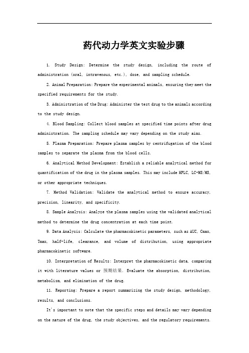
Shows the relative wavelengths of the electromagnetic waves of three different colors of light (blue, green and red) with a distance scale in micrometres along the x-axis.
Since light is an oscillation it is not affected by travelling through static electric or magnetic fields in a linear medium such as a vacuum. However in nonlinear media, such as some crystals, interactions can occur between light and static electric and magnetic fields — these interactions include the Faraday effect and the Kerr effect.
Electromagnetic radiation is classified according to the frequency of its wave. In order of increasing frequency and decreasing wavelength, these are radio waves, microwaves, infrared radiation, visible light, ultraviolet radiation, X-rays and gamma rays (see Electromagnetic spectrum). The eyes of various organisms sense a small and somewhat variable window of frequencies called the visible spectrum. The photon is the quantum of the electromagnetic interaction and the basic "unit" of light and all other forms of electromagnetic radiation and is also the force carrier for the electromagnetic force.
药代动力学英文实验步骤
药代动力学英文实验步骤1. Study Design: Determine the study design, including the route of administration (oral, intravenous, etc.), dose, and sampling schedule.2. Animal Preparation: Prepare the experimental animals, ensuring they meet the specified requirements for the study.3. Administration of the Drug: Administer the test drug to the animals according to the study design.4. Blood Sampling: Collect blood samples at specified time points after drug administration. The sampling schedule may vary depending on the study aims.5. Plasma Preparation: Prepare plasma samples by centrifugation of the blood samples to separate the plasma from the blood cells.6. Analytical Method Development: Establish a reliable analytical method for quantification of the drug in the plasma samples. This may include HPLC, LC-MS/MS, or other appropriate techniques.7. Method Validation: Validate the analytical method to ensure accuracy, precision, linearity, and specificity.8. Sample Analysis: Analyze the plasma samples using the validated analytical method to determine the drug concentration at each time point.9. Data Analysis: Calculate the pharmacokinetic parameters, such as AUC, Cmax, Tmax, half-life, clearance, and volume of distribution, using appropriate pharmacokinetic software.10. Interpretation of Results: Interpret the pharmacokinetic data, comparing it with literature values or预期结果. Evaluate the absorption, distribution, metabolism, and elimination of the drug.11. Reporting: Prepare a report summarizing the study design, methodology, results, and conclusions.It's important to note that the specific steps and details may vary depending on the nature of the drug, the study objectives, and the regulatory requirements.Additionally, adhering to ethical guidelines and following Good Laboratory Practice (GLP) or equivalent standards is essential throughout the experimental process. If you have specific questions or need more detailed information, please provide the specific drug and study context, and I will do my best to assist you further.。
- 1、下载文档前请自行甄别文档内容的完整性,平台不提供额外的编辑、内容补充、找答案等附加服务。
- 2、"仅部分预览"的文档,不可在线预览部分如存在完整性等问题,可反馈申请退款(可完整预览的文档不适用该条件!)。
- 3、如文档侵犯您的权益,请联系客服反馈,我们会尽快为您处理(人工客服工作时间:9:00-18:30)。
a r X i v :h e p -p h /0612094v 2 31 A u g 2007Drell-Yan processes,transversity and light-cone wavefunctionsB.Pasquini,M.Pincetti,S.BoffiDipartimento di Fisica Nucleare e Teorica,Universit`a degli Studi di Pavia and INFN,Sezione di Pavia,Pavia,Italy(Dated:February 2,2008)The unpolarized,helicity and transversity distributions of quarks in the proton are calculated in the overlap representation of light-cone wavefunctions truncated to the lowest order Fock-space components with three valence quarks.The three distributions at the hadronic scale satisfy an interesting relation consistent with the Soffer inequality.Results are derived in a relativistic quark model including evolution up to the next-to-leading order.Predictions for the double transverse-spin asymmetry in Drell-Yan dilepton production initiated by proton-antiproton collisions are presented.Asymmetries of about 20–30%are found in the kinematic conditions of the PAX experiment.PACS numbers:13.88.+e.Hb,13.85.Qk,12.39.Ki I.INTRODUCTIONAt the parton level the quark structure of the nucleon is described in terms of three quark distributions,namely the quark density f 1(x ),the helicity distribution g 1(x )(also indicated ∆f (x )),and the transversity distribution h 1(x )(also indicated δf (x )).The first two distri-butions,and particularly f 1(x ),are now well established by experiments in the deep-inelastic scattering (DIS)regime and well understood theoretically as a function of the fraction x of the nucleon longitudinal momentum carried by the active quark [1].Information on the last leading-twist distribution is missing on the experimental side because h 1(x ),being chiral odd,decouples from inclusive DIS and therefore can not be measured in such a traditional source of information.Nevertheless some theoretical activity has been developed in calcu-lating h 1(x )and finding new experimental situations where it can be observed (for a recent review see Ref.[2]).Among the different proposals the polarized Drell-Yan (DY)dilepton production was recognized for a long time as the cleanest way to access the transversity dis-tribution of quarks in hadrons[3,4,5,6].As a matter of fact,in pp and p¯p DY collisions with transversely polarized hadrons the leading order(LO)double transverse-spin asymmetry of lepton-pair production involves the product of two transversity distributions,thus giving direct access to them.However,such a measurement is not an easy task because of the tech-nical problems of maintaining the beam polarization through the acceleration.The recently proposed experimental programs at RHIC[7]and at GSI[8]have raised renewed interest in theoretical predictions of the double transverse-spin asymmetry in proton-(anti)proton collisions with dilepton production[9,10,11].As reviewed in[2],h1(x)has been calculated in a variety of models,including relativistic bag-like,chiral soliton,light-cone,and spectator models.In all these calculations the an-tiquark transversity is rather small and the d-quark distribution turns out to have a much smaller size than the u-quark distribution.In this paper h1(x)and the other quark distributions are derived within the framework of the overlap representation of light-cone wavefunctions(LCWFs)originally proposed in Refs.[12]to construct generalized parton distributions(GPDs).A Fock-state decomposi-tion of the hadronic state is performed in terms of N-parton Fock states with coefficients representing the momentum LCWF of the N partons.Direct calculation of LCWFs from first principles is a difficult task.On the other hand,constituent quark models(CQMs) have been quite successful in describing the spectrum of hadrons and their low-energy dy-namics.At least in the kinematic range where only quark degrees of freedom are effective, it is possible to assume that at the low-energy scale valence quarks can be interpreted as the constituent quarks treated in CQMs.In the region where they describe emission and reabsorption of a single active quark by the target nucleon,quark GPDs are thus linked to the non-diagonal one-body density matrix in momentum space and can be calculated both in the chiral-even and chiral-odd sector[13,14,15].Sea effects represented by the meson cloud can also be integrated into the valence-quark contribution to GPDs[16].In such an approach the quark distributions,being the forward limit of GPDs,are related to the diagonal part of the one-body density matrix in momentum space.The paper is organized as follows.In Sect.II the overlap representation of LCWFs is briefly reviewed with the aim of linking the parton distributions to CQMs.Results for the three valence quark distributions are discussed at the hadronic scale and after evolution up to the next-to-leading(NLO)in Sect.III.The application to double transverse-spinasymmetry in DY collisions is presented in Sect.IV,andsomeconclusions are drawn in the final Section.II.THE OVERLAP REPRESENTATION FOR PARTON DISTRIBUTIONSIn the overlap representation of LCWFs[12]the proton wave function with four-momentum p and helicityλis expanded in terms of N-parton Fock-space components, i.e.|p,λ = N,β [d x]N[d2 k⊥]NΨ[f]λ,N,β(r)|N,β;k1,...,k N ,(1) whereΨ[f]λ,N,βis the momentum LCWF of the N-parton Fock state|N,β;k1,...,k N .The integration measures in Eq.(1)are defined as[d x]N=Ni=1dx iδ 1−N i=1x i ,[d2 k⊥]N=1M0ω1ω2ω32,and the matrices D1/2µiλi(R cf(k i))are given by the spin-space representation of the Melosh rotation R cf,D1/2λµ(R cf(k))= λ|R cf(xM0, k⊥)|µ= λ|m+xM0−i σ·(ˆ z× k⊥)(m+xM0)2+ k2⊥|µ .(4)In this approach the ordinary(unpolarized)parton distributions offlavor q[17]can be recovered taking into account that in this case the Melosh rotation matrices combine to the identity matrix:f q1(x)= λiτi3 j=1δτjτq [dx]3[d k⊥]3δ(x−x j)|Ψ[f]λ({x i},{ k⊥,i};{λi},{τi})|2,(5) where the helicityλof the nucleon can equivalently be taken positive or negative.Analo-gously,the following simple expressions are obtained for the polarized quark distribution of flavor q[14]g q1(x)= λiτi3 j=1δτjτq sign(λj) [dx]3[d k⊥]3δ(x−x j)|Ψ[f]+({x i},{ k⊥,i};{λi},{τi})|2,(6) and for the quark transversity distributions h q1(x)[15]:h q1(x)= λt iτi3 j=1δτjτq sign(λt j) [dx]3[d k⊥]3δ(x−x j)|Ψ[f]↑({x i},{ k⊥,i};{λt i},{τi})|2,(7) whereλt i is the transverse-spin component of the quark and,as usual,the transversity basis for the nucleon spin states is obtained from the helicity basis as follows:|p,↑ =12(|p,+ +|p,− ),|p,↓ =12(|p,+ −|p,− ).(8) Expressions(5),(6)and(7)exhibit the well known probabilistic content of parton distri-butions.Eq.(5)gives the probability offinding a quark with a fraction x of the longitudinal momentum of the parent nucleon,irrespective of its spin orientation.The helicity distri-bution g q1(x)in Eq.(6)is the number density of quarks with helicity+minus the number density of quarks with helicity−,assuming the parent nucleon to have helicity+.The transversity distribution h q1(x)in Eq.(7)is the number density of quarks with transverse polarization↑minus the number density of quarks with transverse polarization↓,assuming the parent nucleon to have transverse polarization↑.In the instant form it is convenient to separate the spin-isospin component from the space part of the proton wave function and to assume SU(6)symmetry,i.e.Ψ[c]λ({ k i},{λi},{τi})=ψ( k1, k2, k3)Φλτ(λ1,λ2,λ3,τ1,τ2,τ3),(9) whereΦλτ(λ1,λ2,λ3,τ1,τ2,τ3)=12 Φ0λ(λ1,λ2,λ3)Φ0τ(τ1,τ2,τ3)+Φ1λ(λ1,λ2,λ3)Φ1τ(τ1,τ2,τ3),(10)with the superscripts0and1referring to the total spin or isospin of the pair of quarks1 and2.Thus wefindf q1(x)= 2δτq1/2+δτq−1/2 [dx]3[d k⊥]3δ(x−x3)|ψ({x i},{ k⊥,i})|2,(11)g q1(x)= 43δτq−1/2 [dx]3[d k⊥]3δ(x−x3)|ψ({x i},{ k⊥,i})|2M,(12)h q1(x)= 43δτq−1/2 [dx]3[d k⊥]3δ(x−x3)|ψ({x i},{ k⊥,i})|2M T,(13) where[15,18]M=(m+x3M0)2− k2⊥,3(m+x3M0)2+ k2⊥,3,(15) and the expectation values on the normalized nucleon momentum wavefunction of the con-tribution coming from Melosh rotations satisfy2 M T = M +1.(16) Therefore the following relations holdh u1(x)=13f u1(x),h d1(x)=16f d1(x),(17)which are compatible with the Soffer inequality[19]:|h q1(x)|≤13f u1and h d1=g d1=−1axial-vector coupling constant G A and giving also a good agreement with the experimental nucleon electroweak form factors in a large Q2range.Furthermore,we note that SU(6) symmetry is broken in the LCWFΨ[f][21]as a consequence of the transformation(3).The distributions in Eqs.(11),(12)and(13)are defined at the hadronic scale Q20of the model.In order to make predictions for experiments,a complete knowledge of the evolution up to NLO is indispensable.According to Ref.[22]we assume that twist-two matrix elements calculated at some low scale in a quark model can be used in conjunction with QCD perturbation theory.Starting from a scale where the long-range(confining)part of the interaction is dominant,we generate the perturbative contribution by evolution at higher scale.In the case of transversity the Dokshitzer-Gribov-Lipatov-Altarelli-Parisi(DGLAP) Q2evolution equation[23]is simple.In fact,being chirally odd,the quark transversity distributions do not mix with the gluon distribution and therefore the evolution is of the non-singlet type.The leading order(LO)anomalous dimensions werefirst calculated in Ref.[24]but promptly forgotten.They were recalculated by Artru and Mekhfi[25].The one-loop coefficient functions for Drell-Yan processes are known in different renormalization schemes[26,27,28].The NLO(two-loop)anomalous dimensions were also calculated in the Feynman gauge in Refs.[29,30]and in the light-cone gauge[31].The two-loop splitting functions for the evolution of the transversity distribution were calculated in Ref.[31].The LO DGLAP Q2evolution equation for the transversity distribution h1(x)was derived in Ref.[25]and its numerical analysis is discussed in Refs.[32,33].A numerical solution of the DGLAP equation for the transversity distribution h1(x)was given at LO and NLO in Refs.[34,35].In Ref.[34]the DGLAP integrodifferential equation is solved in the variable Q2with the Euler method replacing the Simpson method previously used in the cases of unpolarized[36]and longitudinally polarized[37]structure functions.In the present analysis the FORTRAN code of Ref.[34]has been applied within thecode at NLO is computed by solving the NLO transcendental equation numerically,ln Q2β0αs+β1β0αs+β14π=1β20ln ln(Q2/Λ2NLO)0.20.40.60.8100.20.40.60.81x f 1u 00.20.40.60.8100.20.40.60.81x f 1d 00.511.500.20.40.60.81NS x x f 1u 00.20.40.60.8100.20.40.60.81NS x x f 1d Figure 1:Evolution of the parton distribution for the u (left panel)and d (right panel)quark.Inthe lower panels starting from the hadronic scale Q 20=0.079GeV 2(upper curve),LO non-singletdistributions are shown at different scales (Q 2=5GeV 2,solid lines;Q 2=9GeV 2,dashed lines;Q 2=16GeV 2,dotted lines)together with NLO distributions at Q 2=5GeV 2(dot-dashed lines).LO and NLO total distributions are shown in the upper panels with the same line convention.The parametrization of Ref.[39]NLO evolved at 5GeV 2is also shown by small stars.In any case the Soffer inequality (18)at each order is always satisfied by the three quark distributions calculated with the LCWFs of the present model (see Fig.4).In contrast,saturation of the Soffer bound,i.e.assuming|h q 1(x )|=100.20.400.20.40.60.81 x x g 1u -0.05000.20.40.60.81x x g 1d 00.5100.20.40.60.81NS x x g 1u -0.2-0.1000.20.40.60.81NSx x g 1d Figure 2:The same as in Fig.1,but for the helicity distribution.evolution.In fact,starting at the hadronic scale with the transversity distribution given by Eq.(21),the result of LO and NLO evolution diverges from that obtained when calculating the transversity according to Eq.(21)after separate evolution of f 1and g 1.Since the two sides of Eq.(21)give different results under evolution,in model calculations the choice of the initial hadronic scale is crucial.This fact should put some caution about the possibility of making predictions with the transversity distribution guessed from f 1and g 1as,e.g.,in the case of the double transverse-spin asymmetry in DY processes (see Refs.[10,11]and Fig.7below).A similar situation occurs when the transversity distribution is derived from f 1and g 1according to the relations (17),with the difference that these relations are exact at the hadronic scale when only valence quarks are involved.00.20.40.60.8100.250.50.751NS x x h 1u-0.3-0.2-0.1000.250.50.751NS x x h 1d Figure 3:Evolution of the transversity distribution for the u (left panel)and d (right panel)quark.Starting from the hadronic scale Q 20=0.079GeV 2(upper curve),LO non-singlet distributions areshown at different scales (Q 2=5GeV 2,solid lines;Q 2=9GeV 2,dashed lines;Q 2=16GeV 2,dotted lines)together with NLO distributions at Q 2=5GeV 2(dot-dashed lines).IV.THE DOUBLE TRANSVERSE-SPIN ASYMMETRYIn order to directly access transversity via Drell-Yan lepton pair production one has to measure the double transverse-spin asymmetry A T T in collisions between two transversely polarized hadrons:A T T =dσ↑↑−dσ↑↓q e 2q f q 1(x 1,Q 2)f ¯q 1(x 2,Q 2)+(1↔2) ,(23)where e q is the quark charge,Q 2the invariant mass square of the lepton pair (dimuon),and00.511.500.250.50.751NS x x h 1u -0.3-0.2-0.1000.250.50.751NSx x h 1d Figure 4:The transversity distribution obtained with the LCWFs of the present model (thin lines)compared with the Soffer bound,Eq.(21),(thick lines)for the u (left panel)and d (right panel)quark .Solid lines for the results at the hadronic scale Q 20=0.079GeV 2,the dashed lines obtainedby NLO evolution at Q 2=9GeV 2,respectively.x 1x 2=Q 2/s where s is the Mandelstam variable.The quantity a T T is the spin asymmetry of the QED elementary process q ¯q →ℓ+ℓ−,i.e.a T T (θ,φ)=sin 2θat RHIC very small,no more than a few percents[33,42,45].A more favorable situation is expected by using an antiproton beam instead of a proton beam[8,9,10,11,46].In p¯p DY the LO asymmetry A p¯p T T is proportional to a product of quark transversity distributions from the proton and antiquark distributions from the antiproton which are connected by charge conjugation,e.g.h u/p 1(x)=h¯u/¯p1(x).(25)Therefore one obtainsA p¯p T T=a T Tq e2q h q1(x1,Q2)h q1(x2,Q2)+h¯q1(x1,Q2)h¯q1(x2,Q2)2lnx10.10.20.30.40.500.20.40.60.81 1.2yA T T /a T T Figure 5:The double transverse-spin asymmetry A p ¯p T T /a T T calculated with the parton distributionsof the present model as a function of the rapidity y at different scales:Q 2=5GeV 2,solid line;Q 2=9GeV 2,dashed line;Q 2=16GeV 2,dotted line.This result confirms the possibility of measuring the double transverse-spin asymmetry under conditions that will be probed by the proposed PAX experiment.In such conditions,assuming the LO expression (26)for the observed asymmetry one could gain direct infor-mation on the transversity distribution following previous analyses [9,10,11],where thequark densities f q,¯q 1(x,Q 2)are taken from the GRV98parametrizations [39].The resultingtransversity distributions could be compared with model predictions.According to this strategy,with the present model the antiquark distributions h ¯q 1(x,Q 2)are identically vanishing and h q 1(x,Q 2)contains only valence quark contributions.Assuminga negligible sea-quark contribution the corresponding asymmetry would thus give directaccess to h q 1(x,Q 2)and would look like that shown in Fig.6.The results indicate a strongQ 2dependence suggesting moderate values of Q 2,e.g.Q 2=5to 10GeV 2,in order to have an appreciable asymmetry of about 10–20%at the proposed PAX experiment at GSI [8].It is remarkable that,contrary to the result of Ref.[9],in the present model Q 2evolution produces a decreasing LO asymmetry with increasing Q 2as a consequence of the opposite00.10.20.300.20.40.60.81yA T T /a T T Figure 6:The same as in Fig.5but assuming the GRV98[39]quark density.00.20.400.20.40.60.81yA T T /a T T Figure 7:The double transverse-spin asymmetry A p ¯p T T /a T T as a function of the rapidity y at Q 2=5GeV 2and s =45GeV 2.Solid curve:calculation with h 1obtained with the LCWFs of the present model.Dashed curve:calculation with an input h 1=1Q2dependence of the theoretical h1and the phenomenological f1.In fact,in the range of x-values explored by the chosen kinematic conditions(x≥0.3)h1with its valence quark contribution has a larger fall-offwith Q2than the GRV98f1as shown in Fig.1.Furthermore, one may notice that with the present model a much lower asymmetry is predicted than with the chiral quark-soliton model[9]and even lower than the phenomenological analysis of Refs.[10,11].In general,one can anticipate upper and lower limits for the theoretical asymmetry depending on the upper and lower bounds that the transversity has to satisfy.The saturated Soffer bound(21),i.e.h1=1(g1+f1)(dashed curve)or assuming2the nonrelativistic approximation h1=g1(dotted curve),with f1and g1calculated in the present model.The difference between the dotted and solid curves gives an estimate of the relativistic effects in the calculation of h1.On the other side,the model calculation with an input h1satisfying Eq.(17)leads to an asymmetry much lower than in the case of the saturated Soffer bound.V.CONCLUSIONSThe unpolarized,helicity and transversity distributions of quarks in the proton are calcu-lated in the overlap representation of light-cone wavefunctions truncated to the lowest order Fock-space components with three valence quarks.The light-cone wavefunctions have been defined making use of the correct covariant connection with the instant-form wavefunctions used in any constituent quark model.The quark distributions have been evolved to leading order and next-to-leading order of the perturbative expansion with the remarkable result that NLO effects are rather small compared to LO.The three distributions at the hadronicscale satisfy an interesting relation consistent with the Soffer inequality.In particular,the transversity distribution has been used to predict the double transverse-spin asymmetry in dilepton production with Drell-Yan collisions between transversely polarized beams of protons and antiprotons.As a function of rapidity the asymmetry calculated in the model is about30%for s=45GeV2,slightly increasing with Q2.In contrast,when using phe-nomenological unpolarized quark distributions together with the transversity distribution derived in the present model,the asymmetry turns out to be smaller than previous predic-tions,e.g.about10–20%at Q2=5GeV2and s=45GeV2,and rapidly decreases with increasing Q2.This is due to the different Q2dependence of the involved distributions in the allowed range of x values.As the transversity is unknown experimentally,this sensitivity to Q2is an important argument for future experiments.The present results suggest the possibility of measurable asymmetries at moderate values of Q2in the kinematic conditions of the proposed PAX experiment,thus obtaining direct access to the quark transversity distribution.[Note added in the proof:During the revision process a phenomenological analysis of available data appeared[48]and the transversity distributions for up and down quarks were shown to have opposite sign and a smaller size than their positivity bounds in agreement with the results of the present model.]AcknowledgementsThis research is part of the EU Integrated Infrastructure Initiative Hadronphysics Project under contract number RII3-CT-2004-506078.[1] mpe and E.Reya,Phys.Rep.332,1(2000);R.L.Jaffe,hep-ph/9710465;M.Dittmar et al.,hep-ph/0511119.[2]V.Barone,A.Drago,and P.G.Ratcliffe,Phys.Rep.359,1(2002);V.Barone and P.G.Ratcliffe,Transverse Spin Physics,World Scientific,Singapore,2003. [3]J.P.Ralston and D.Soper,Nucl.Phys.B152,109(1979).[4]J.L.Cortes,B.Pire,and J.P.Ralston,Z.Phys.C55,409(1992).[5]Xiangdong Ji,Phys.Lett.B284,137(1992).[6]R.L.Jaffe and Xiangdong Ji,Phys.Rev.Lett.67,552(1991);Nucl.Phys.B375,527(1992).[7]G.Bunce,N.Saito,J.Soffer,and W.Vogelsang,Ann.Rev.Nucl.Part.Sci.50,525(2000).[8]P.Lenisa,F.Rathmann et al.(PAX Collaboration),Technical proposal for Antiproton–ProtonScattering Experiments with Polarization,hep-ex/0505054.[9] A.V.Efremov,K.Goeke,and P.Schweitzer,Eur.Phys.J.C35,207(2004).[10]M.Anselmino,V.Barone,A.Drago,and N.N.Nikolaev,Phys.Lett.B594,97(2004).[11]V.Barone,A.Cafarella,C.Corian`o,M.Guzzi,and P.G.Ratcliffe,Phys.Lett.B639,483(2006).[12]M.Diehl,Th.Feldmann,R.Jakob,and P.Kroll,Nucl.Phys.B596,33(2001);S.J.Brodsky,M.Diehl,and D.S.Hwang,Nucl.Phys.B596,99(2001).[13]S.Boffi,B.Pasquini,and M.Traini,Nucl.Phys.B649,243(2003).[14]S.Boffi,B.Pasquini,and M.Traini,Nucl.Phys.B680,147(2004).[15] B.Pasquini,M.Pincetti,and S.Boffi,Phys.Rev.D72,094029(2005).[16] B.Pasquini and S.Boffi,Phys.Rev.D73,094001(2006).[17]S.J.Brodsky and G.P.Lepage,in:A.H.Mueller(ed.),Perturbative Quantum Chromodynam-ics,World Scientific,Singapore,1989,p.93;S.J.Brodsky,H.-Ch.Pauli,and S.S.Pinsky,Phys.Rep.301,299(1998).[18]I.Schmidt and J.Soffer,Phys.Lett.B407,331(1997);Bo-Qiang Ma,I.Schmidt,and J.Soffer,Phys.Lett.B441,461(1998).[19]J.Soffer,Phys.Rev.Lett.74,1292(1995).[20] F.Schlumpf,J.Phys.Nucl.Part.Phys.G20,237(1994).[21] F.Cardarelli and S.Simula,Phys.Rev.C62,065201(2000).[22]R.L.Jaffe and G.G.Ross,Phys.Lett.B93,313(1980).[23]Yu.L.Dokshitzer,JETP(Sov.Phys.)46,641(1977)[Zh.Exsp.Teor.Fiz.73,1216(1977)];V.N.Gribov and L.N.Lipatov,Sov.J.Nucl.Phys.15,438,675(1972)[Yad.Fiz.15,781, 1218(1972)];L.N.Lipatov,Sov.J.Nucl.Phys.20,94(1975)[Yad.Fiz.20,181(1974)];G.Altarelli and G.Parisi,Nucl.Phys.B126,298(1977).[24] F.Baldracchini,N.S.Craigie,V.Roberto,and M.Socolovsky,Fortschr.Phys.29,505(1981).[25]X.Artru and M.Mekhfi,Z.Phys.C45,669(1990).[26]W.Vogelsang and A.Weber,Phys.Rev.D48,2073(1993).[27] A.P.Contogouris,B.Kamal,and J.Merebashvili,Phys.Lett.B337,169(1994).[28] B.Kamal,Phys.Rev.D53,1142(1996).[29] A.Hayashigaki,Y.Kanazawa,and Y.Koike,Phys.Rev.D56,7350(1997).[30]S.Kumano and M.Miyama,Phys.Rev.D56,R2504(1997).[31]W.Vogelsang,Phys.Rev.D57,1886(1998).[32]V.Barone,Phys.Lett.B409,499(1997).[33]V.Barone,T.Calarco,and A.Drago,Phys.Lett.B390,287(1997).[34]M.Hirai,S.Kumano,and M.Miyama,m.111,150(1996).[35] A.Cafarella and C.Corian`o,m.160,213(2004).[36]M.Miyama and S.Kumano,m.94,185(1996).[37]M.Hirai,S.Kumano,and M.Miyama,m.108,35(1996).[38]T.Weigl and W.Melnitchouk,Nucl.Phys.B465,267(1996);M.Traini,V.Vento,A.Mair,and A.Zambarda,Nucl.Phys.A614,472(1997);B.Pasquini,M.Traini,and S.Boffi,Phys.Rev.D71,034022(2005).[39]M.Gl¨u ck,E.Reya,and A.Vogt,Eur.Phys.J.C5,468(1998).[40]M.Gl¨u ck,E.Reya,M.Stratmann,and W.Vogelsang,Phys.Rev.D63,094005(2001);J.Bl¨u mlein and H.B¨o ttcher,Nucl.Phys.B636,225(2002);Y.Goto et al.,Phys.Rev.D62,034017(2000);Int.J.Mod.Phys.A18,1203(2003).[41]O.Martin,A.Sch¨a fer,M.Stratmann,and W.Vogelsang,Phys.Rev.D57,3084(1998).[42]O.Martin,A.Sch¨a fer,M.Stratmann,and W.Vogelsang,Phys.Rev.D60,117502(1999).[43] C.Bourrely and J.Soffer,Nucl.Phys.B423,329(1994).[44] C.Bourrely and J.Soffer,Nucl.Phys.B445,341(1995).[45]V.Barone,T.Calarco,and A.Drago,Phys.Rev.D56,527(1997).[46] A.Bianconi and M.Radici,Phys.Rev.D72,074013(2005).[47]H.Shimizu,G.Sterman,W.Vogelsang,and H.Yokoya,Phys.Rev.D71,114007(2005).[48]M.Anselmino,M.Boglione,U.D’Alesio,A.Kotzinian,F.Murgia,A.Prokudin,and C.Turk,Phys.Rev.D75,054032(2007).。