2008-SEM-2
纤维素、木质素含量对生物质热解气化特性影响的实验研究

样品
嚣弈:雾辜:弄耋萎:某薷霎
∞
舳
∞
∞
加
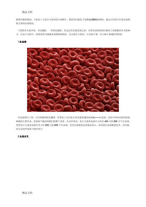
每次实验生物质样品量为5 mg左右,分别在 N2与C02气氛下进行热解和气化实验.实验原料 分林业植物松木,农业植物稻壳、稻草、棉杆、玉米
0 松木
稻草
棉轩玉米芯稻壳”蔗渣
图1生物质中纤维索,木质素以及酸性可溶有机物含量
Fig.1 Cellulose and lig】nin contents in several types of biomass
关键词生物质;纤维索;木质索;热解;气化
中图分类号:TK6
文献标识码,A
文章编号;0253--231X(2008)10-1771-04
EFFECT oF CELLULoSE AND LIGNIN CoNTENT oN PYRoIⅣSIS
AND GASIFICATIoN CHARACTERISTICS FoR SEVERAL
第29卷第10期 2008年10月
工程热物理学报
JOURNAL OF ENGINEERING THERMOPHYSICS
V01.29,No.10 0ct..2008
纤维素、木质素含量对生物质热解气化 特性影响的实验研究
吕当振姚洪王泉斌 李志远 彭钦春刘小伟 徐明厚
(华中科技大学煤燃烧国家重点实验室, 湖北武汉 430074)
收稿日期:2007-12-14;修订日期:2008-07-14 基金项目;教育部科学技术研究重点资助项目(No.107074);国家自然科学基金资助项目(No.50721005,No.50325621) 作者简介:吕当振(1982~),男,湖北武汉人.博士研究生,主要从事生物质热解气化特性及其应用研究。
摘要 本文采用化学方法测定了六种生物质中纤维素和木质索的含量,通过热重研究了实际生物质及用纤维素、木质 素按一定比例混合模拟生物质的热解和气化特性,并结合电子扫描电镜(SEM)对焦样进行了微观形貌分析。结果表明s 在本文所选择的生物质中纤维素的含量高于木质索,两者一般在55%一85%和10%一35%.生物质热解分为纤维素热解 和木质素分解两个阶段,对应于气化过程中挥发份析出和焦炭气化。在热解过程中,首先纤维素发生热解皂现快速失重过 程,接着木质索缓慢热解.实验发现生物质中纤维素含量越高,热解反应速率就越大;反之,木质素含量越高,热解反应 速率越小.通过对焦形貌与气化研究,发现气化特性与生物质中纤维索和木质索的含量有着密切联系.因此纤维索、木质 素含量是影响生物质热解气化特性的重要因素之一.
离港系统09

配载操作流程图
航班建立 油量输入 开始配载
预配输入
实配定位 打印舱单 关闭发报
机组修正 平衡检查
结束配载
§5-2 基本系统指令
一、进入系统
进入生产系统 : >$$OPEN TIPJ 进入测试系统: >$$OPEN TIPE2
工作区显示 DA 请签到注册,工作号为888,密码321321,工 作级91,工作组CAN001
建立航班的T-CARD BF:T
T-CARD:航班数据放在系统中一个形式
指令功能: 建立/显示/修改航班的数据信息
工作号级别必须为96级;
在FDC系统中,航班由T1-CARD和T2-CARD构成;
T1-CARD描述航班的一般特性如航班类型、布局等,对每 一个航班至少有一个T1行;
T2-CARD描述航班航程上每一城市的到达、起飞及登机时 间等信息;
章节构成
§5-1 §5-2
离港系统简介
基本系统指令
§5-3
工作流程及相关指令
§5-1 离港系统简介
一、系统介绍
计算机离港控制系统(Departure Control System),简称DCS,是中国民航引进美国 UNISYS公司的航空公司旅客服务大型系统。
旅客值机控制系统(CKI)
SO 退出工作区
>SO
§5-2 基本系统指令
三、公用信息指令
功能帮助系统 HELP
国家/ 城市/ 机场信息查询 CNTD
计算功能
日期/ 时间查询与对比显示
长度、重量、温度各进制间的转换
翻页功能
功能帮助系统HELP
1Cr18Ni9Ti与1Cr13不锈钢的焊接试验[1]
![1Cr18Ni9Ti与1Cr13不锈钢的焊接试验[1]](https://img.taocdn.com/s3/m/1e02552eb4daa58da0114a27.png)
为 1Cr13 马氏体不锈钢母材拉伸断口微观组织形 貌 ,断口中韧窝小且多 , 属于韧性断 裂. 图 2c 为 1Cr18Ni9Ti 奥氏体不锈钢和 1Cr13 马氏体不锈钢焊 接接头拉伸断口微观组织形貌 ,韧窝和撕裂棱混合 共存 ,但撕裂棱在断口中所占的比例较小 ,仍属于韧 性断裂. 断口中 ,韧窝的大小和深度各不相同 ,韧窝 的大小和深度相差悬殊 ,这与焊接 HAZ 晶粒大小不 均匀以及析出第二相粒子的数量 、形状和分布有 关[4] . 2. 2 焊接接头力学性能 2. 2. 1 焊接接头的显微硬度
86
焊 接 学 报
第 30 卷
从图 1 中可以看出 ,在靠近奥氏体区 ,得到奥氏 体组织. 在马氏体侧形成板条状马氏体[3] ,因为马 氏体不锈钢含铬量高 ,淬透性好 ,在焊缝金属从液态 降温时 ,接近母材 ,冷却速度快 ,空冷时形成了马氏体 组织. 在焊接接头的熔合区得到典型的柱状晶组织. 2. 1. 2 断口 SEM 观察及分析
5
缝区
2. 3. 1 焊接接头的交流阻抗对比分析 图 4 为焊接接头各区域的交流阻抗谱. 从图 4
中可以看出 ,阻抗弧由小到大的试样编号为 2 号 , 5 号 ,4 号 ,3 号 ,1 号 ,阻抗弧越小 ,相对应的低频阻 抗幅值越小 ,所以腐蚀速度越快 ,所以腐蚀率由大到 小的变化顺序为 2 号 ,5 号 ,4 号 ,3 号 ,1 号. 这是由 于在靠近奥氏体 、马氏体母材的热影响区 ,得到单相 的奥氏体 、马氏体组织 ,耐蚀性相对于双相或多相组 织要强 ;在焊缝区 ,马氏体不锈钢和奥氏体不锈钢焊 接熔合的过程中 ,两种不锈钢所含的镍 Ni ,Cr ,Ti 等 元素扩散转移 ,化学成分不均匀性使焊缝区可能得 到双相或多相的混合组织 ,从而使焊缝的耐腐蚀性
(整理)电子显微镜SEM拍摄的人体图片
据国外媒体报道,下面这十五张令人惊异的人体图片,都是用扫描电子显微镜(SEM)拍摄的,通过它们你可以更近地观察人体的内部情况。
下面将从头部开始,穿过胸腔,一直到达腹腔,经过这次自我发现之旅,让你切身体验到扫描电子显微镜的非凡影响力。
在这个过程中,你将看到当细胞受到肿瘤侵扰时,会出现什么情况,以及卵子第一次与精子相遇时的情景。
1.红血球从这张图片上看,它们很像肉桂色糖果,但事实上它们是人体里最普通的血细胞——红血球。
这些中间向内部凹陷的细胞的主要任务,是将氧气输送到我们的整个身体。
在女性体内,每立方毫米血液中大约有400万到500万个红血球,男性每立方毫米血液中有大约500万到600个红血球。
居住在海拔较高的地区的人,体内的红血球数量更多,因为他们生活的环境氧气相对更少。
2.头发分叉经常修剪和良好的护理,可避免像这张图片上出现发梢分叉的现象。
3. 普尔基涅神经元在大脑里的1000亿个神经元中,普尔基涅神经元是体积最大的。
这些细胞是小脑皮层里的运动协调大师。
接触酒精、锂等有毒物质、患有自身免疫性疾病、存在孤独症和神经退行性疾病(Neurodegenerative disease)等遗传变异,都会对人类的普尔基涅神经元造成消极影响。
4.耳毛细胞这张图片看起来好像是在耳朵里面对耳毛细胞进行近距离观察时拍摄的。
耳毛细胞的主要功能是发现对声震作出反应时产生的机械运动。
5.从视神经中伸出的血管这张照片显示的是血管从黑色视盘中伸出。
视盘是个盲点,因为视网膜的这个区域没有光感细胞,视神经和视网膜血管从眼睛后面的这个部位伸出去。
6.舌头上的味蕾这张彩色图片上显示的是舌头上的一个味蕾。
人舌上大约拥有10000个味蕾,味蕾所感受的味觉可分为甜、酸、苦、咸四种。
其他味觉,如涩、辣等都是由这四种融合而成的。
7.牙釉质要有一口亮丽牙齿,经常刷牙非常有必要,因为牙齿表面的牙釉质看起来就像“煮熟的老玉米”。
8.血液凝块还记得你刚刚看到的形状统一的红血球图片吗?这张图看起来像是红血球粘在了粘性网上,形成血液凝块。
【北京市自然科学基金】_扫描电镜(sem)_基金支持热词逐年推荐_【万方软件创新助手】_20140729
科研热词 推荐指数 硫化 2 cuins2薄膜 2 高温 1 镍 1 铂微粒 1 钝化 1 金红石 1 输尿管 1 超声深滚 1 表面涂层 1 表面改性 1 荧光原位杂交 1 自润滑 1 胞外多聚物 1 聚(癸二酸-丙三醇-柠檬酸)酯 1 耐蚀性能 1 组织相容性 1 纳米银颗粒 1 纳米化 1 纳米二氧化锆 1 纳米二氧化硅 1 级次结构 1 离子 1 疲劳性能 1 电化学传感器 1 甲醛 1 生物降解 1 生物相容性 1 热开裂 1 激光熔覆 1 溶剂热 1 水泥浆体 1 氮气载流量 1 氧 1 染色 1 显微组织 1 支架 1 摩擦性能 1 微观结构劣化 1 微球 1 导电性能 1 好氧颗粒污泥 1 太阳能电池 1 太阳电池 1 喷墨导电墨水 1 同步脱氮除磷 1 合金 1 化学镀 1 光催化 1 ti6al4v合金 1 ni-cu-p 1 mos2 1
2012年 序号 1 2 3 4 5 6 7 8 9 10 11 12 13 14 15 16 17 18 19 20 21 22 23
科研热词 静电纺丝 聚吡咯 电化学性能 钯-镍双金属 表面活性剂 葡萄糖氧化酶 芯片变黑 聚对苯二甲酸丁二醇酯 群落分布 纳米纤维 絮凝-纳米纤维填料法 系统发育 氨氧化细菌 染料废水 扫描电镜 微区分析 工艺参数 失效机理 发光二极管 厌氧氨氧化菌 光学器件 pet纳米纤维 canon反应器
科研热词 扫描电镜 静电纺丝技术 阴极粉末 阴极 铝酸盐 铁氧体 钯-镍双金属 超音速等离子 超疏水 超滤 触角 裂纹 聚吡咯 纳米金 纳米纤维 等离子喷涂 磁性 硬度 石墨烯 电纺丝 电化学性能 电化学共还原 热膨胀系数 热导率 滚动角 液相共沉淀法 涂层表征 涂层 浸润性 接触角 接受液 抗水解性能 感器 性能 微结构 对苯二酚 复合纳米纤维膜 喷雾干燥法 南美斑潜蝇 十二烷基苯磺酸钠 准分子激光 体外透皮试验 乙醇 两步氢气还原 xrd sicp/cu复合材料 sem pzt(锆钛酸铅) pbtio3涂层 ito薄膜
现代化学分析方法(仅供参考)
现代化学分析⽅法(仅供参考)SEM 和TEM 统称为电⼦显微镜扫描电镜测试样品表⾯形貌,⽽透射电镜测试内部形貌观察,或者晶体结构分析,特别是微区(微⽶、纳⽶)的像观察和结构分析SEM不能做磁性材料,TEM得是液态样品显微镜放⼤倍数受所⽤波长限制。
电⼦显微镜使⽤电⼦作为光束来观察物体内部或表⾯的结构。
普通光学显微镜是⽤可见光来观察物体的。
由于电⼦的波长远⼩于可见光的波长,所以前者的极限分辨率远⾼于后者的极限分辨率。
“Collect”栏设定扫描次数⼀般是设置16或者32都可以,多扫⼏次为了准确⼀点,⼀般没啥关系为什么减⼩激光器的功率可以减弱荧光对拉曼散射的⼲扰?减⼩激光功率,被激发的分⼦少了,产⽣的荧光跃迁⾃然就少了产⽣荧光所需要的激发能量⾼,产⽣拉曼所需的激发能量低,所以降低激光功率对荧光影响更⼤荧光对拉曼⼲扰问题在拉曼光谱中,通常斯托克斯线的强度⼤于反斯托克斯线,⼀般我们选⽤斯托克斯线部分。
但荧光会严重⼲扰斯托克斯线⽽不⼲扰反斯托克斯线,对能产⽣荧光的试样只能损失灵敏度选反斯托克斯线。
室温时处于基态振动能级的分⼦很少,Anti-stocke线也远少于stocks线。
温度升⾼,反斯托克斯线增加。
从由光学介质和荧光组成的系统来看,Stokes过程和反Stokes过程都是熵不断增⼤的过程。
虽然在反斯托克斯荧光制冷过程中光学介质的熵要减⼩.但由荧光带⾛的熵更⼤。
介质中熵的变化△SM是⼀个很重要的量。
正是由于熵的符号决定了在反斯托克斯过程中不可能产⽣激光。
相关内容还是要掌握的,⽐如什么是stocks和anti-stocks等什么类型的数据属于⼆维数据?荧光分光光度计的⽐⾊⽫为什么需要四⾯透光如果在⼀条直线上那是测吸光度的荧光分光光度计⼊射光源和检测器的⽅向是垂直的这样在垂直⽅向上就不可能有⼊射光⽽激发的荧光在四个⽅向上都有在垂直⽅向上检测⼲扰最⼩所以四⾯透光荧光光谱适⽤低温,是为了增加驰豫作⽤,提⾼灵敏度。
【浙江省自然科学基金】_扫描电镜(sem)_期刊发文热词逐年推荐_20140811
科研热词 推荐指数 表征 2 改性 2 增韧 2 高能球磨 1 静电纺丝 1 降解 1 锌镍合金电镀碱性异常共沉积耐蚀性 1 钛合金 1 钙钛矿型复合氧化物 1 荧光性能 1 草酸 1 脂质体 1 聚苯并噁嗪环氧端基甲基苯基硅油1 聚苯并噁嗪 1 聚电解质微囊 1 纳米铜/石蜡/膨胀石墨 1 纳米棒 1 纳米sio2 1 纤维素 1 稀土掺杂 1 稀土 1 碳酸钙 1 硼酸镍 1 硬度 1 相结构 1 生物相容性 1 环氧端基甲基苯基硅油 1 热性能 1 水热合成 1 氧-氮-碳三元共渗 1 柠檬酸-溶胶凝胶法 1 显微组织 1 接枝 1 层层自组装 1 多柔比星 1 复合材料 1 固载 1 固相法 1 化合物层 1 包覆 1 力学性能 1 分散性 1 共沉淀法 1 光催化剂 1 光催化 1 催化活性 1 催化 1 一维纳米复合材料 1 zinc-nickel alloy, electroplating, 1 alkaline, anom tio2 1 sno2/fe3o4 1 sno2 1
53 54 55 56 57 58 59 60 61 62 63 64 65 66 67 68 69 70 71 72 73 74 75 76 77
2011年 科研热词 聚苯乙烯 黑色素精制 鱿鱼墨 高铁含量 高能球磨 高比表面积 颗粒形态 静电纺 阻燃 铁磁形状记忆合金 钯催化剂 金属间化合物 金属元素分析 透射电镜(tem) 进化 路易斯酸 超临界二氧化碳发泡 超临界co2发泡 血红细胞 膨胀性:温敏性 聚酰胺胺树枝状大分子 聚离子液体 聚磷酸三聚氰胺 羟丙基纤维素 结构表征 纳米铜/石蜡/pvp 纳米sio2 纤维 紫外-可见光吸收 空间网络 稳定性 稀土 离子-电子混合导体 磁熵变 磁感生应变 磁性纳米复合材料 硬度 电子结构 甲基丙烯酸丁酯 激光熔覆 激光技术 水滑石 水产动物 有序介孔材料 接枝改性 择优取向 扫描电镜(sem) 成核剂 微波引诱燃烧 形态特征 弹塑性性能 季戊四醇 推荐指数 2 1 1 1 1 1 1 1 1 1 1 1 1 1 1 1 1 1 1 1 1 1 1 1 1 1 1 1 1 1 1 1 1 1 1 1 1 1 1 1 1 1 1 1 1 1 1 1 1 1 1 1
金属镁粒钝化处理的试验研究

表 1 铁水脱硫用钝化镁的技术标准
化学成分 ,Wt %
物理指标
活性镁 S
粒度 堆比重 燃点 阻燃时间 1273 K
H2O
mm g·cm - 3
K
s
≥90. 0 ≤0. 002 < 0. 5 0. 2~1. 0 ≥0. 73 ≥853
> 11
收稿日期 :2008 - 05 - 25
镁粒钝化处理一般采用化学反应法 、表面覆盖 法和熔融离心成型法 。其中化学反应法能生成较致 密的反应产物薄膜层 ,钝化层均匀 ,钝化效果好 ,工 艺简单 ,应用最为广泛〔1~4〕。本文采用化学反应法 对金属镁粒进行钝化处理 ,通过正交试验 ,研究了钝 化剂组分及工艺参数对镁粒钝化效果的影响 。
1. 3 试样检测分析
镁粒钝化效果的首要指标是阻燃时间 ,因此 ,首 先对正交试验得到试样进行阻燃时间的测定 ,得到 最佳阻燃时间的钝化剂和钝化工艺 。钝化镁粒阻燃 时间的测定使用管式电炉 。将电炉的炉温恒定在 1273 K ,取少量试样放在样勺上 ,推入管式电炉 ,记 录试样进入炉膛到开始燃烧所需要的时间 。每个试 样重复测试 3 次~4 次 ,取平均值即为该试样的阻 燃时间 。
然后用最佳阻燃时间的试样进行燃点和活性镁 验证检测 。钝化镁燃点的测定使用综合热重分析仪 ( ZETZSCH STA 449C) 。取试样约 20mg ,置入热分 析仪内 ,选用空气气氛 ,升温速度为 10 K/ min 。测定 试样的重量变化曲线 ( T G) 和放热速度变化曲线 (DSC) 。当镁粒发生燃烧时 ,试样的重量会明显增
© 1994-2009 China Academic Journal Electronic Publishing House. All rights reserved.
- 1、下载文档前请自行甄别文档内容的完整性,平台不提供额外的编辑、内容补充、找答案等附加服务。
- 2、"仅部分预览"的文档,不可在线预览部分如存在完整性等问题,可反馈申请退款(可完整预览的文档不适用该条件!)。
- 3、如文档侵犯您的权益,请联系客服反馈,我们会尽快为您处理(人工客服工作时间:9:00-18:30)。
Structural Engineering and Mechanics, Vol. 29, No. 2 (2008) 155-169155A MOM-based algorithm for moving force identification:Part II – Experiment and comparative studiesLing YuKey Lab of Disaster Forecast and Control in Engineering, Ministry of Education of the People’s Republic of China (Jinan University), Guangzhou 510632, P. R. ChinaDepartment of Civil and Structural Engineering, The Hong Kong Polytechnic UniversityHong Kong, P. R. ChinaT ommy H.T. Chan†School of Urban Development, Faculty of Built Environment & Engineering, Queensland University ofTechnology, GPO Box 2434, Queensland 4001, AustraliaDepartment of Civil and Structural Engineering, The Hong Kong Polytechnic UniversityHong Kong, P. R. ChinaJun-hua ZhuKey Lab of Disaster Forecast and Control in Engineering, Ministry of Education of the People’s Republic of China (Jinan University), Guangzhou 510632, P. R. ChinaChangjiang River Scientific Research Institute, Wuhan 430010, P. R. China(Received August 30, 2006, Accepted August 7, 2007)Abstract. A MOM-based algorithm (MOMA) has been developed for moving force identification from dynamic responses of bridge in the companion paper. This paper further evaluates and investigates the properties of the developed MOMA by experiment in laboratory. A simply supported bridge model and a few vehicle models were designed and constructed in laboratory. A series of experiments have then been conducted for moving force identification. The bending moment and acceleration responses at several measurement stations of the bridge model are simultaneously measured when the model vehicle moves across the bridge deck at different speeds. In order to compare with the existing time domain method (TDM), the best method for moving force identification to date, a carefully comparative study scheme was planned and conducted, which includes considering the effect of a few main parameters, such as basis function terms, mode number involved in the identification calculation, measurement stations, executive CPU time, Nyquist fraction of digital filter, and two different solutions to the ill-posed system equation of moving force identification. It was observed that the MOMA has many good properties same as the TDM, but its CPU execution time is just less than one tenth of the TDM, which indicates an achievement in which the MOMA can be used directly for real-time analysis of moving force identification in field. Keywords:moving force identification; method of moments (MOM); bridge loads; time domain method (TDM); dynamic responses.†Ph.D., Corresponding author, E-mail: tommy.chan@.au156Ling Yu, Tommy H.T. Chan and Jun-hua Zhu1. IntroductionThe moving force identification is a fundamental problem in the bridge engineering (Olsson 1991). The importance of this problem has attracted much attention during the last two decades due to the large increase in the proportion of heavy vehicles and high-speed vehicles in highway and railway traffic (Y u and Chan 2005, Cebon 1987, Cantineni 1992). Accurate identification of moving forces during operation is vital for cost effective design and maintenance of bridges since this can not only lead to a great reliance on numerical simulation based upon analytical models but also dramatically reduce the need for more expensive and time consuming experimental testing (Chan and O’Conner 1990, Y u and Chan 2002).In recent years, a series of identification methods have been successively proposed and merged into a moving force identification system (MFIS) (Y u 2002), and some further comparative studies on the effects of different parameters on the system have also been carried out and critically investigated in laboratory (Chan et al. 2000, Y u and Chan 2003), in which the time domain method (TDM) (Law et al. 1997) has been proved to be the best one in all of the identification methods and applied successfully to a field study (Chan et al. 2000). Although all these methods can identify moving forces with acceptable accuracy, each method has its own merits, limitations and disadvantages. For example, the TDM has higher identification accuracy but it is time consuming. Moreover, the TDM often provides a significant fluctuation at the beginning and the end of time histories of identified moving forces due to the nature of ill-posed problem of moving force identification (Tikhonov and Arsenin 1977, Santantamarina and Fratta 1998, Law et al. 2001). Based on the method of moments (MOM) and the theory of moving force identification, a MOM-based algorithm (MOMA) has been proposed for identifying the time-varying vehicle axle loads from the dynamic responses of a bridge in the companion paper (Y u et al. 2008). Some numerical simulation results have shown that the MOMA has higher identification accuracy and robust noise immunity as well as an acceptable solution to the ill-conditioning problem to some extent. However, these results are all from the numerical simulation at all, and the best tool to assess the new method should be through experiments in laboratory or field tests (Harris and Sabnis 2000, Bilello et al. 2004).As its companion paper (Y u et al. 2008), this paper aims to further evaluate and critically investigate the MOMA and compare it with the existing TDM through experiments in laboratory based on a comparative study. A bridge-vehicle system is designed and fabricated in laboratory, a series of experiments have been conducted for moving force identification under different conditions. The bending moment and acceleration responses at some measurement stations of the bridge model are simultaneously measured when the model vehicle moves across the bridge deck at different speeds. In contrast to the TDM, a carefully comparative study scheme was planned and conducted, which includes considering the effect of a few main parameters, such as basis function terms, mode number involved in the identification calculation, measurement stations, CPU execution time, Nyquist fraction of digital filter, and two different solutions to the ill-posed system equation of moving force identification. Some conclusions are finally made.2. Experiments in laboratoryAfter the proposed MOMA method had been evaluated through numerical simulations in theA MOM-based algorithm for moving force identification: Part II 157 companion paper (Y u et al. 2008), a series of experiments were further conducted in laboratory for assessing the robustness of MOMA.2.1 Experimental setupBoth the model car and model bridge deck were designed and fabricated in the laboratory as shown in Fig. 1. Here, a beam model was used to model the tested bridge and a car model was constructed from available materials in the laboratory. The model car had two axles at a spacing of 0.55 m and was mounted on four rubber wheels. The static mass of the whole vehicle was 12.1kg in which the mass of the rear wheel was 3.825 kg. The model bridge deck consisted of a main beam, a leading beam and a trailing beam. The leading and trailing beam were attached at both ends of the main beam, in which the leading beam was used for initiating the motion and speeding up the car so that the car could reach a constant speed when it approaches the main beam. The trailing beam was used for decelerating the car. The main beam, with a span of 3.678m long and a 101mm×25mm uniform cross section, was simply supported. It was made from a solid rectangular mild steel bar with a density of 7335kg/m3 and a flexural stiffness EI=29.97kN·m2. A U-shape aluminum track was glued to the upper surface of the main beam as a guide way for the model-car. The first three theoretical natural frequencies of the main beam bridge were calculated as 4.5Hz, 18.6Hz and 40.5Hz respectively. The tested bridge model is fabricated, as shown in Fig. 2. Sensors used in the experiments include photoelectric sensors, strain gauges and accelerometers. Seven photoelectric sensors were mounted beside the beams to measure and check the uniformity of the moving speed of the model car. Seven strain gauges and three accelerometers were equally spaced mounted on the lower surface of the main beam to measure the bridge response when the model car was moving across it. A system calibration of the strain gauges was carried out before the actual testing program by adding masses at the middle of the main beam. The calibration factors for each of the strain gauges are listed in Table 1.A data acquisition system was prepared to acquire the dynamic responses of the bridge model induced by the model car crossing the bridge. The system comprises of a sensor element, a conditioning element, a converting element and a processing element. During the test, the model car was pulled along by a string wound around the drive wheel of an electric motor. The speed of the motor could be adjusted in order to get a specific car speed. A 14-channel tape recorder was employed to record the response signals. The first seven channels were used for logging the bending moment response signals from the strain gauges, channels 8-10 were for the acceleration response signals from the accelerometers, and channel 11 was connected to the photoelectric sensors. In addition, the response signals from channels 1-7 and 11 were also recorded simultaneously into a PC for easy analysis in situ. The software Global Lab from the Data Translation was used for data acquisition and analysis in the laboratory tests. Under all the studied cases, the data were acquiredFig. 1 Experimental model designed for laboratory tests158Ling Yu, Tommy H.T. Chan and Jun-hua ZhuFig. 2 Experimental model fabricated in the laboratoryTable 1 Calibration factors of strain gaugesStation no.Channel no.Strain gauge no.(L)(Nm/V) 1111L/8289.02222L/8285.23333L/8285.94444L/8296.65555L/8297.76666L/8297.17777L/8298.4A MOM-based algorithm for moving force identification: Part II 159 in a sampling frequency of 1000Hz, which is higher than the practical demands. The data sequences were sampled again to form a new sequence at a lower sampling frequency. When deciding the sampling frequency to form a new data sequence, the new sampling was checked if it fulfilled the Nyquist rate requirement (Proakis and Manolakis1996). Before exporting the measured data in ASCII format for identification, the Bessel IIR digital filter with low-pass characteristics was implemented as cascaded second order systems. The Nyquist fraction value was chosen to be 0.03 and 0.05 respectively for different requirement of frequency band needed.2.2 Experimental resultsThe measured bending moment and acceleration responses of the bridge were recorded under three sets of vehicle speed, i.e., 5, 10 and 15 Units. After acquiring the data, the vehicle speed was calculated and the uniformity of the speed was checked. If the speed was stable, the experiment was repeated fives times under each speed case to check whether the properties of both the structure and the measurement system had changed or not. If no significant change was found, the corresponding recorded data was accepted for identification of the moving forces. The identification of each case and check of the uniformity of vehicle speed is shown in Table 2.All the response data recorded into the PC and the Tape recorder under each case were checked and found that they were all very good and could be used to identify the moving forces on the bridge. Two typical measured responses of bending moments at seven equally spaced strain gauges and acceleration responses at three equally spaced accelerometers, which were installed on the lower surface of the bridge, are plotted in Fig. 3. All filtered data corresponding to all scheduled cases were stored in the personal computer and exported in ASCII format for moving force identification in two-force study cases.Table 2 Experimental measurement cases and vehicle speed calculationCases Speed of vehicle at different segments of bridge span (m/s) Speed Name12345Average5 Unit U5-10.69750.71970.72260.70840.71300.71224 U5-20.72080.73400.70000.70290.72670.71688 U5-3*0.70730.75240.73120.72050.71480.72524 U5-40.7540.75690.72460.71860.72010.73484 U5-50.73060.74170.71050.70380.69920.7171610 Unit U10-1 1.2715 1.3978 1.4690 1.5124 1.2921 1.38856 U10-2 1.4067 1.2073 1.0063 1.1002 1.1393 1.17196 U10-3 1.1968 1.1478 1.1058 1.1204 1.1158 1.13732 U10-4 1.0943 1.0939 1.0719 1.0598 1.1144 1.08686 U10-5 1.1407 1.1354 1.1073 1.1113 1.1003 1.1190015 Unit U15-1 1.4755 1.5417 1.4935 1.4718 1.5372 1.50394 U15-2 1.505 1.5267 1.5132 1.5421 1.5291 1.52322 U15-3 1.2463 1.2656 1.2798 1.2650 1.2386 1.25906 U15-4 1.6793 1.7424 1.7692 1.7426 1.5318 1.69306 U15-5 1.5202 1.5608 1.5815 1.5082 1.5594 1.54602*Notes: Case U5-3 means the third test when the vehicle runs at the speed of 5 Unit.160Ling Yu, Tommy H.T. Chan and Jun-hua Zhu3. Comparative studiesThe moving force identification includes many parameters, which are the critical parts in the identification processing. The comparative study is to investigate the effects of several main parameters on the MOMA, and further compared with the existing TDM. The parameters studied include basis function terms, mode number, measurement stations, CPU execution time, the Nyquist fraction value, and various solutions to the ill-posed problem of system equation on the moving force identification (Y u et al . 2008). For practical reasons, the parameters were studied one at a time. The procedure was to examine each parameter in studied cases and to isolate the case with the highest accuracy for the corresponding parameter.3.1 Accuracy assessmentAs the true moving forces are unknown in practice, the identification accuracy of moving forces cannot be evaluated directly, but can be assessed indirectly through the measured and rebuilt responses. The latter are calculated from the identified moving forces as a forward problem in the structural dynamics. Therefore, the accuracy, called relative percentage error (RPE), is quantitatively defined as below(1)Here, R measured indicates the measured response and R rebuilt the rebuilt response respectively.In the comparative studies being reported here, the results were based on the measurements of bending moments. The results associated with the measured accelerations will be reported separately. The identified forces were first calculated from the bending moment responses at all seven measuring stations. The rebuilt responses were then computed accordingly from the identified forces. The RPE values between the rebuilt and measured bending moment responses at each station were finally tested for validation. The maximum acceptable RPE value adopted here is 10% (Chan et al. 2000).RPE R measured R rebuilt–∑R measured----------------------------------------------100%×=Fig. 3 Typical measured responses of bridge due to moving vehicleA MOM-based algorithm for moving force identification: Part II 1613.2 Effect of basis function termsBasis function plays an important role in the identification of moving loads for the MOMA. To assess the effect of basis function number (BFN) on the MOMA, the other parameters are chosen as following: the mode number of the bridge involved in the moving force identification is equal to four (MN = 4), the sampling frequency is equal to 200 Hz (f s = 200 Hz), the speed of vehicle is 15 Units (case U15-2 in Table 2, c = 1.52322 m/s), and the measurement bending moments at seven stations are all selected, i.e. the sensor number of locations are seven (N l = 7). Fig. 4 plots the effect of BFN on the MOMA with Legendre basis function and one with Fourier basis function, in which the BFN increases up to 600, while other parameters MN = 4, f s = 200, c = 15 Units, N l = 7 were not changed for any of the cases.Fig. 4 illustrates that both the RPE values tend to be reduced and finally to be close to each other when BFN increases. The major difference between them is that the rate of reduction is obviously different. If the Fourier basis functions are used, the RPE values are dramatically reduced to the lowest value and then kept the lowest constant after the basis function term is equal to about 100 or more for each case. However, if the Legendre basis functions are adopted, the process of RPE reduction will be clearly slower than the Fourier case. It is noted that the identification accuracy is stable and kept the highest when the corresponding basis function terms are increased up to be more than 400, even 500.Fig. 5 gives a comparison on the time histories of moving forces identified by the TDM andFig. 4 Effect of basis function number (BFN) on MOMA162Ling Yu, Tommy H.T. Chan and Jun-hua ZhuMOMA respectively when the basis function terms are equal to 500 for Legendre polynomials and 100 for Fourier series respectively. Here, the LMOMA result is from the MOMA when the basis function is Legendre polynomials. Similarly, the FMOMA result is from the basis function of Fourier series. From the figure, it can be seen that the identified results from the MOMA are in agreement with the TDM results. Moreover, the MOMA results are better than the TDM results,particularly for the moment at the beginning and the end of time history of two moving forces as well as the moment at the accessing and exiting of the vehicle on the bridge. For the front axle in Fig. 5(a), the moment of the second axle of the vehicle accessing into the bridge is at about 0.35second, the TDM result has a big jump, but the MOMA result is smoother and better than the TDM. At the end of time history of the moving force at the front axle, the FMOMA is better than the LMOMA and both of them are further better than the TDM result since the FMOMA result does not result in an unreasonable jump. For the rear axle in Fig. 5(b), similarly, at about 2.05second, the exiting moment of the front axle of the vehicle, the MOMA result is better than the TDM. At the beginning of time history of identified moving force at the rear axle, the FMOMA is better than the LMOMA and further better than the TDM. It can draw a conclusion from above that the MOMA can provide a more reasonable and acceptable solution to the ill-posed problem of the moving force identification to some extent when the MOMA is adopted to identify the moving forces from the bridge responses, especially for the FMOMA, the MOMA with the basis function of Fourier series.Further, Table 3 lists the RPE values of the MOMA and the TDM respectively. It shows that the identification accuracy of the MOMA is consistent with that of the TDM. In addition, when the Fourier basis function is adopted, the FMOMA forms a coefficient matrix with a small dimension in the system equation and results in a small CPU execution cost due to the small BFN , so the MOMA has higher computation efficiency. Therefore, it is only considered the solutions of MOMA with Fourier basis function (FMOMA) in the following studies, from the point of view ofcomputation efficiency as well as the identification accuracy.Fig. 5 Comparison on moving forces identified by TDM and MOMATable 3 Comparison of TDM and MOMA Method 1234567TDM 6.72 3.31 2.43 2.99 2.58 3.96 6.29MOMA6.823.292.442.962.593.976.33A MOM-based algorithm for moving force identification: Part II 1633.3 Effect of mode numbersFor both the TDM and MOMA, the case of f s = 200 Hz, c = 15 Units, N l = 7 was chosen and not changed. The mode number was varied from MN = 2 to MN = 8. Fig. 6 plots typical effects of the mode number on the two identification methods. Obviously, the effect of mode number on both MOMA and TDM is not so significant. With the mode number increase, the RPE curve decrease firstly and then increases, and the better case is MN = 4 for both methods.3.4 Effect of measurement stationsThe case MN = 4, f s = 200 Hz, c = 15 Units is chosen for studying the effects of number and locations of measurement stations. The N l were set to 3, 4, 5 and 7 respectively while other parameters were not changed for any cases. Table 4 lists a comparison on the RPE values by the TDM and MOMA respectively. It shows that there is no significant difference between the TDM and MOMA results for each case under the same condition. The effect of measurement stations on the MOMA is identical with that of TDM. In addition, Fig. 7 illustrates a comparison on the effect of measurement stations on the MOMA. It can be found that the more the number of measurementstations, the better the identified results for the MOMA as a general conclusion.Fig. 6 Effect of mode number (MN) on TDM and MOMATable 4 Effect of Measurement Stations on TDM and MOMA Statio TDMMOMA N l = 3N l = 4N l = 5N l = 7N l = 3N l = 4N l = 5N l = 71*** 6.72*** 6.822* 1.58 2.37 3.31* 1.58 2.37 3.293 1.50 1.95 2.16 2.43 1.50 1.95 2.15 2.444 1.67* 2.87 2.99 1.71* 2.88 2.965 1.71 2.26 2.45 2.58 1.70 2.26 2.44 2.596* 1.69 2.33 3.96* 1.69 2.35 3.977***6.29***6.33Notes: Symbol * indicates the station is not selected.164Ling Yu, Tommy H.T. Chan and Jun-hua Zhu3.5 Comparison on CPU execution timeThe CPU execution time consists of three parts for both TDM and MOMA, i.e. forming the system coefficient matrix, identifying moving forces and producing the rebuilt responses. The case described here is of MN = 4, f s = 200Hz, c = 15 Units, N l = 7 using a computer with Intel Pentium (R) 4 CPU 2.6GHz 512MB RAM. The total sampling points for bending moment responses at each measurement station are 560 and the total sampling points for each wheel axle force are 483 in the time domain. Therefore, the dimensions of coefficient matrix for TDM are (7×560, 2×483), while the matrix for MOMA are (7×560, 2×101). A detail comparison of the CPU execution time for each part of the TDM and MOMA is listed in Table 5. It shows that both the MOMA and TDM take almost the same time for both of the rebuilding responses and forming the system coefficient matrix. However, the CPU execution time of MOMA is about 6% of TDM for the identifying force process. Hence, the total consuming time of MOMA is only two fifth of that of TDM. Therefore,MOMA is a better and fast method, whether from the point of view of identifying force time or from the total consuming time. This advantage with higher computation efficiency for the MOMA is especially valuable for the on-line real-time analysis of moving force identification in situ.3.6 Effect of nyquist fractionTo filter the high frequency noise of measured response signals, a Bessel IIR digital filter with low pass characteristics was chosen and implemented as a cascaded second order system. Different Nyquist fractions of the filter were chosen for the measured bending moments. The Nyquist fraction is defined as the ratio of cutoff frequency to sampling frequency of dynamic signals. The cutoff frequency may be specified in Hertz relative to the sampling frequency, or as a fraction oftheFig. 7 Effect of measurement stations on moving forces for MOMATable 5 Comparison on executive CPU time (in second)PARTTDM MOMA Forming coefficient matrix 18.21919.907Identifying moving forces 40.359 2.375Rebuilding responses1.063 1.094Total59.64123.376A MOM-based algorithm for moving force identification: Part II165Nyquist frequency. A bigger Nyquist fraction indicates a filtered signal with higher frequency components in the frequency domain.In this section, Nyquist fraction values were first set to 0.03 and 0.05 respectively and then used to filter the data samples recorded at the sampling frequency of 1000 Hz for all the cases. The new data sequence would be formed by sampling again at different rate, for example, f s = 200 Hz as required. To study the effect of Nyquist fraction on identification accuracy, only the Nyquist fraction was changed here, but others parameters MN = 4, f s = 200 Hz, c = 15 Units, N l = 7 were not changed for each case. Table 6 lists the RPE values when the Nyquist fraction changes for both TDM and MOMA respectively. It can be seen that the RPE values increases slightly with the increase in the Nyquist fraction whether from the TDM or MOMA results, which shows that the higher frequency noise has an influence on the identified results when the Nyquist fraction is set to be a higher value. Further, Fig. 8 illustrates the effect of Nyquist fractions on the identified moving forces for MOMA. It shows that the magnitude of identified forces increases and the identified forces have some clear higher frequency components when the Nyquist fraction has a higher value.Therefore, the Nyquist fraction should be selected properly to reasonably identify the moving vehicle loads on bridge.3.7 Effects of different solutionsIf the parameters MN = 4, f s = 200 Hz, c = 15 Units, N l = 7 were not changed for each case in this section, only two solutions, i.e., SVD and Regularization solutions, were adopted to solve the over-determined set of system equations respectively. Table 7 lists a comparison on the RPE values by both TDM and MOMA when the two solutions are adopted. It can be found from the Table 7Table 6 Effect of Nyquist fractions on MOMA Nyquist fraction 12345670.03 6.72 3.31 2.43 2.99 2.58 3.96 6.296.82 3.29 2.44 2.96 2.59 3.97 6.330.056.43 2.79 2.74 3.14 3.16 4.74 6.606.522.802.763.133.184.746.64Notes: the underlined values are from MOMA, others from TDM.Fig. 8 Effect of Nyquist fractions on moving forces for MOMA166Ling Yu, Tommy H.T. Chan and Jun-hua Zhuthat the RPE values from each of two identification methods are increased a little bit when the Regularization solution is adopted in contrast to the SVD solution. This is because the SVD solution provides a solution to make the residual of Ax-b minimum for a system equation of Ax = b, but the Regularization solution provides a balance between the residual of Ax-b and the norm of x, i.e. it makes the summation of the residual and the norm minimum. So the Regularization solution is often not the minimum residual solution. When the system equation is ill-conditioning or there is noise in the response data vector of b, the SVD solution would be often unstable in the sense that small perturbations in the responses would result in large deviation from their true solution even a whole wrong solution (Law et al.2001). However, the Regularization solution can be used to stabilize the unbounded solution since it provides a bound to the ill-posed problem on moving force identification.Moreover, it can be seen from Table 7 that the regularization method has less influence on the TDM results in contrast to the MOMA results. Figs. 9 and 10 are the L-shape curves for selection of regularization parameters for TDM and MOMA respectively (Busby and Trujillo 1997, Hansen 1992, Hansen and O’Leavy 1993). From above two figures, it can be found that the regularization parameter is equal to 0.0096145 for the TDM but 0.16483 for the MOMA. The lower the regularization parameter, the better the fitting extent of solution to the responses, however, the lessTable 7 Comparison on RPE values by SVD and Regularization solutionsMethodsStation1234567TDM 6.72 3.31 2.43 2.99 2.58 3.96 6.296.73 3.31 2.43 2.99 2.58 3.95 6.30MOMA 6.82 3.29 2.44 2.96 2.59 3.97 6.337.08 3.29 2.47 2.76 2.67 3.82 6.75 Notes: the underlined values are from Regularization solution, others from SVD solution.Fig. 9 L-shape curve for selecting regularization parameter for TDM Fig. 10 L-shape curve for selecting regularization parameter for MOMAA MOM-based algorithm for moving force identification: Part II 167the bound constrains to the norm of solution. Therefore, the regularization method has a better efficiency to the MOMA than the TDM.Fig. 11 illustrates a comparison on the identified moving forces due to the two solutions for MOMA. Basically, the regularization results are in agreement with the SVD results except for the moment at the beginning and the end of time histories of moving forces as well as the moment at the accessing and exiting of vehicle on bridge in the time history of moving forces. It shows that the fluctuation of identified moving forces can be effectively bounded at the moment mentioned above if the Regularization solution is adopted to solve the system equation for MOMA. The identified results by the Regularization solution are obviously improved. They are clearly better than the results by the SVD solution and more reasonable in practice. 4. ConclusionsIn this paper, a series of experiments have been carried out in the laboratory for evaluation on the MOM-based algorithm (MOMA), a new developed method for identification of moving forces from the responses of a bridge. A comparative study has been performed to assess the effect of some parameters on the new method using the measured data in laboratory. These parameters mainly include the basis function terms of both Legendre polynomials and Fourier series, mode number of bridge involved in the identification calculation, the measurement stations, the CPU execution time of identification method, Nyquist fraction of digital filter, and the two different solutions to the over-determined system equation. Some conclusions can be made as following. (1) The MOMA is correct, reasonable and suitable for moving force identification from the bridge responses. It is successful to identify the moving vehicle loads on bridges using the MOMA in laboratory. (2)Comparing with the existing time domain method (TDM), the MOMA has same good advantages as the TDM. Both the MOMA and TDM have similarly optimum selection criteria for the common parameters, such as mode number, measurement stations and Nyquist fraction. Some conclusions for the TDM are also suitable for the MOMA. (3) The basis function terms play an important role in the MOMA. The different patterns of basis function can lead to different computation efficiency,and the basis function number has been obviously affected the identification accuracy in practice.The more the basis function number is, the higher the MOMA identification accuracy is, but leading to longer CPU execution time. If the basis function number was chosen properly, the CPU time would be greatly shortened. Therefore, the basis function should be properly selected andappropriately determined in order to keep the MOMA more effective. (4) The MOMA can improveFig. 11 Effect of two solutions on moving forces for MOMA。