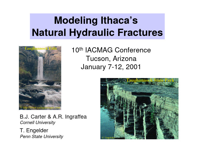
Modeling Ithaca’s natural hydraulic fractures

1INRODUCTIONHydraulic fractures occur naturally in the Earth’s crust. These range in size from mm as small pres-sure partings to km as magmatic dike intrusions. Ithaca, New York, which lies in the heart of the Fin-ger Lakes region, is a great place to see intermedi-ate-scale natural hydraulic fractures. Glaciation and erosion have led to large outcrops of middle and up-per Devonian clastic rocks. These rocks have ex-perienced two major orogenic events in addition to uplift and erosion all of which have left a pattern of brittle fracture in the rocks as seen today. A brief geological history of the area is necessary to set the stage for the discussion of natural hydraulic frac-tures in these rocks.Outcrops within the Finger Lakes are part of the Devonian Catskill Delta Complex, a clastic wedge that is more than 2 km thick in the Finger Lakes re-gion. The complex was deposited on a continental shelf with an open sea to the south and consists of layers of black shales, gray shales, silstones and sandstones, and an occasional limestone. Uplift ac-companying the Acadian orogeny to the east pro-vided a large source of sediment for the clastic wedge that was prograding into the Appalachian Ba-sin. Deposition rates reached 170m per Ma. At the close of the Paleozoic, during the Pennsylvanian and Permian, the Alleghanian orogeny caused wide-spread folding, faulting and jointing in eastern North America. This was the last major orogeny to affect this part of the continent.Engelder and others (see Engelder et al. 2000) have studied the joints and other geologic features within the Catskill Delta Complex for many years. There is an abundance of evidence that indicates that many of these joints developed as natural hydraulic fractures caused by abnormally high fluid pressures. The Alleghanian orogeny also left a unique imprint as many joints show a clockwise sequence in re-sponse to the reorientation of stress as the African continent collided with North America.There is a significant body of literature that de-scribes the joints and tries to interpret their origin and formation (e.g. Pollard & Aydin 1988). How-ever, there have been few numerical simulations to illustrate the theorized processes. The aim of this paper is to examine various components of these joints using numerical simulations to determine whether current formation theories are reasonable or valid.2GEOLOGIC EVIDENCE OF NATURAL HYDRAULIC FRACTURES AND STRESS ROTATIONSThe current theories of joint formation in the Cats-kill Delta Complex depend upon visual inspection of many joints and joint sets (Engelder et al. 2000). The first bit of evidence comes from the surface morphology of many of the joint surfaces in the silt-stone.Modeling Ithaca’s natural hydraulic fracturesB.J. Carter & A.R. IngraffeaCornell University, Ithaca, NY, USAT. EngelderPenn State University, University Park, PA, USAABSTRACT: Joints within the Catskill Delta complex are believed to be natural hydraulic fractures and abundant indirect evidence supports this claim. The indirect evidence is based on many observations of joint surface morphology and joint spacing among other features. The Alleghanian orogeny left a unique imprint on the joint surfaces also, indicating a rotating horizontal compressive stress field. Numerical simulations il-lustrate that the formation and propagation of the joints can be described by hydraulic fracturing mechanisms. The numerical simulations include hydraulic fracture propagation from sedimentary structures at layer inter-faces and fracture twisting in response to the reorientation of the remote stress field after initial joint propaga-tion.Cracks tend to start at points of higher stress con-centration (McConaughy & Engelder 2000). In the case of sedimentary beds, the largest stress concen-trations are in the form of concretions, fossils, rip-ples, groove casts, and similar features. Figure 1 shows a joint surface in the Ithaca Formation silt-stone that starts at a groove cast, a location where the siltstone penetrates the shale layer, formed dur-ing erosion of the muddy substrate and deposition of the silt. The figure also shows the plumose surface morphology of the joint surface. The plumose struc-tures and the related arrest lines are well described by Bahat & Engelder (1984). Barbs, the darkened lines in Figure 1, radiate from the plume axis and indicate the direction of fracture growth. Arrest lines mark the termination of crack propagation in-crements. Natural hydraulic fractures do not have a steady supply of fluid (Lacazette & Engelder 1992). As the crack propagates, the pressure decays and the crack arrests until the pressure builds up again.Figure 1. Plumose joint surface starting from a groove cast.It can also be seen in Figure 1 that the fracture initially stays within the siltstone layer. It has been found that in sedimentary basins where the horizon-tal stress is less than the vertical, the shale layers have a higher horizontal stress than the siltstones (Evans et al. 1989, Warpinski 1989). Assuming that the pore pressure is the same in both the shale and siltstone layers, then the fractures would form in the siltstones first. This will be more evident in the next figure.The difference in horizontal stress leads to joint-ing in the siltstones followed by jointing in the shale. Joints in the shale beds usually start at the edges of existing joints in the siltstone; the joints act as con-duits for the pore fluid. If there is no rotation of the principal horizontal stresses, joints will develop in the shale in plane with those in the sandstone. How-ever, if the horizontal stress does rotate, then en-echelon or fringe cracks will develop (Pollard et al. 1982). Figure 2 shows a set of fringe cracks that start at the interface between the siltstone and shale. These fractures propagate downward. The numer-ous small cracks at the immediate interface reduce to a few large cracks as propagation continues.Figure 2. Multiple en-echelon cracks propagate down from the siltstone-shale interface and are rotated from the parent joint.There are many more features of the joints that offer indirect evidence of natural hydraulic fractures, including joint spacing, slip on open joints, crosscut-ting and abutting relationships, and evidence of a pressure seal that could have led to over-pressurization of the formation. However, it is be-yond the scope of this paper to discuss all of this evidence. Instead, numerical simulations are used to illustrate that natural hydraulic fracturing processes can explain some of the features described herein.3HYDRAULIC FRACTURING SOFTWARE The 3D numerical simulations that are described in the following sections are performed using HY-FRANC3D and accompanying software (Carter et al. 2000a,b). In addition, ANSYS (ANSYS 2000) and FRANC2D (CFG 2000) are used for some 2D analyses.The 3D software consists of OSM, FRANC3D, HYFRANC3D, and BES. OSM is used to create the initial geometric models. FRANC3D is a fracture analysis code with pre- and post-processing capabili-ties. HYFRANC3D builds upon FRANC3D by add-ing a fluid flow module that couples the elastic structural response with fluid flowing in the fracture. BES is a linear elastic boundary element program. BES provides an elastic influence matrix that re-lates the set of unit pressures (p) at the nodes on the crack surface to the elastic displacements (w). The fluid flow formulation is based on the elasticity, lu-brication and continuity equations. For a Newtonian fluid, the stress ahead of the crack front has a 1/3 singularity, as does the fluid pressure inside thecrack (Carter et al. 2000b). Physically, the fluid pressure cannot be singular, thus, a fluid lag must develop at the crack front (Figure 3). The finite ele-ment formulation in HYFRANC3D combines an analytical solution for the pressure and crack open-ing displacement at the crack front with a standard finite element formulation of the lubrication equa-tion for the bulk of the fracture. The analytical solu-tion at the crack front provides an elegant way to overcome the singular behavior and limits the re-quired number of elements at the crack front. Hy-draulic fracture simulation proceeds as a series of crack advance increments, requiring an elastic solu-tion and coupled flow analysis at each step.Figure 3. Crack front region with fluid lag; p is pressure, w is crack opening displacement, V is crack front velocity, σ3 is clo-sure stress and x is the local coordinate axis along the crack.4SIMULATION OF HYDRAULIC FRACTURE PROPAGATION FROM A GROOVE CASTCracks tend to start at pre-existing flaws and points of high stress concentration. The groove cast in Fig-ure 1 is modeled to evaluate the stress intensification and to determine the hydraulic fracture propagation behavior from this location. The intent of these simulations is to show that hydraulic fracture is a plausible mechanism; thus, realistic boundary condi-tions are necessary, but accurate values are not es-sential to provide qualitative results.The numerical model consists of the siltstone layer only. McConaughy & Engelder (2000) de-scribe the difficulties in determining and modeling the correct boundary conditions. They conclude that the interface between the shale and siltstone must al-low slip. To simplify the 3D model, the upper and lower shale layers are notmodeled; a vertical con-straint is applied to the upper surface. A far-field compressive stress is applied in the horizontal direc-tion only; the vertical stress is neglected. The com-pressive stress perpendicular to the crack surface is 50 MPa and the stress parallel to the crack plane is 100 MPa. The elastic modulus is set to 14 GPa and the Poisson’s ratio is set to 0.1.The initial plane strain ANSYS stress analysis clearly shows that the groove cast alters the horizon-tal stress (Fig. 4). A tensile stress is induced at the groove cast. An initial crack is nucleated in the 3D numerical model at this location and hydraulic frac-ture propagation is simulated.Figure 4. ANSYS contours of maximum principal stress around a groove cast in a siltstone layer; tension is positive and values are in MPa.Figure 5 shows the shape of the hydraulic fracture after 17 steps of propagation. The fluid boundary conditions consist of a crack mouth flow rate equal to 1.0e-6 m3/s and zero flow rate at the crack front. These boundary conditions do not match the pre-sumed conditions of periodic fluidpressure build-up, but it is assumed that this will only affect the fracturing time and the surface features. The shape of the fracture to this stage matches that seen in the field reasonably well, although the barbs and arrest lines cannot be reproduced. The simulation can be continued such that the fracture breaks through the upper surface of the silt layer, but this is not com-plete yet.Figure 5. Shape of a hydraulic fracture from a groove cast af-ter 17 steps of propagation.5SIMULATION OF HYDRAULIC FRACTURE IN A ROTATING STRESS FIELDHydraulic fractures in these brittle rocks tend to grow perpendicular to the direction of maximum tension (or minimum compression). If an initial crack is subjected to a rotated stress field, the crack will kink out of the original plane to align itself with the new stress field. The rotation of the stress field induces different modes of deformation on different parts of the crack front. The kinking behavior de-pends on the pressure distribution inside the crack, the geometry of the crack, and the stress and stiff-ness contrasts in the rock layers (Carter et al. 1999). As a simple example, an initial elongated radial crack (emanating from a horizontal borehole) is ori-ented 70°from the maximum horizontal compres-sive stress (Fig. 6). The crack is nucleated in a single layer model with an elastic modulus of 27.6 GPa and a Poisson’s ratio of 0.25. The vertical stress is 69 MPa, the maximum horizontal stress is 62 MPa, and the minimum horizontal stress is 48 MPa. The crack mouth flow rate is set to 0.0795 m3/s.Figure 6. The initial crack shape is 9 m long and 0.3 m deep; σHmax is aligned with the x-axis (not to scale).Hydraulic fracture is simulated and stress inten-sity factors (SIF’s) are computed. Figure 7 shows the distribution of SIF’s along the initial crack front. The mode I values are highest, but there is a signifi-cant mode III component; mode II is significant only at the ends of the crack front. Pollard et al. (1982) provide a relationship between the mode III/I ratio and the number and spacing of en-echelon cracks that form along the crack front. Germanovich (2000) is conducting experiments on glass and brittle plastic to further characterize these relationships.The combination of all three modes is studied less well. However, the HYFRANC3D software allows the crack to propagate while ignoring the mode III SIF. Under these circumstances, the crack front does not break up, although, it quickly shows that it should. Figure 8 shows that the ends of the crack turn to align with σHmax. Most of the crack front is not aligned with σHmax. Instead, “large” ripples can be seen. The ripples are a result of the numerical propagation procedure, which only accounts for modes I and II. As the fracture propagates, the mode II and mode III SIFs increase rather than decrease. Due to the elongated shape, more effort is required to turn the entire crack front as compared to a more circular shape crack (Carter et al, 1999). As the crack front does not break, the combination of modes I and II produces initially minor oscillations in the crack front. These escalate as the crack con-tinues to grow, leading to the ripples.The mode III SIF value in the middle of the crack front reaches 10 MPa⋅√m at the final stage (15th step of propagation) while the mode I value remains rela-tively constant for each step, ranging from 20 to 25 MPa⋅√m along the crack front. Rotation and break up of the crack front is seen in many locations in the Ithaca area; Figure 9 shows a typical example.Figure 7. Mode I, II, and III SIF’s along the crack front; values are in MPa⋅√m.Figure 8. Ignoring mode III SIF during propagation leads to “large” ripples in the crack front indicating it should break up. The ends of the crack turn to align with the stress field.Figure 9. Joint in a siltstone indicating a rotated stress field as the crack surface shows obvious breaks; this might be seen as a set of en-echelon cracks when looking from above.6SIMULATION OF MULTIPLE HYDRAULIC FRACTURESMultiple parallel cracks tend to reduce in number and increase in spacing as they propagate. It is often assumed that the length to spacing ratio should be about 1.0 for a stable system of parallel cracks (Hwang, 1999). Figure 2 shows an example of a large number of closely spaced fractures at the shale-siltstone interface. As the cracks propagate down into the shale, most of the cracks arrest very quickly. Only a few, relatively widely spaced cracks remain at the base of the shale layer. Based on this figure, the length to spacing ratio is significantly greater than 1.0. Hwang (1999) has studied systems of parallel cracks, although not for 3D hydraulic fractures. Both 3D hydraulic fracture simulations and 2D simulations will be performed here.A set of three hydraulic fractures is used to gain insight into the behavior of a system of many paral-lel hydraulic fractures. The initial model is shown in Figure 10. The model is symmetrically constrained. The initial cracks are 1 mm deep and 6.35 mm apart. The crack mouth flow rate is 1.0e-6 m3/s and the material properties are the same as in section 4. In reality, more cracks should be modeled, but the simulations become quite time consuming as more cracks are added; three cracks should provide ade-quate insight.HYFRAN3D computes pressure distributions and crack opening displacements in the 3D fractures along with SIF distributions along the crack front. The usual procedure for growing multiples cracks is to scale the crack growth for all cracks based on the relative values of the stress intensity factors. Using this technique, the 3D hydraulic fractures are propa-gated for 10 steps. Although the mode I SIF for the center crack is slightly less than that for the two outer cracks (14.5 versus 15.2 MPa⋅√m for the initial crack), it continues to propagate. At step 10, the crack length is 10.5 mm. The length to spacing ratio is 1.7 and the center crack shows no signs of arrest-ing based on the relative mode I SIF values, 3.4 ver-sus 3.5 MPa⋅√m for the center and outer cracks re-spectively. Based on Figure 2, one might expect that the length to spacing ratio could be much higher than this. To verify that the crack growth is still sta-ble, 2D simulations are performed.FRANC2D is able to compute SIF’s, energy re-lease rates, and rates of energy release rates. The lat-ter allows the program to decide whether crack growth is stable and to decide which of the cracks are arrested. Although FRANC2D does not simulate fluid flow, a static pressure distribution of arbitrary shape can be applied to the crack surfaces (edges). It was shown previously (Carter et al, 1999) that if the correct pressure distribution, based on the 3D fluid flow analysis in HYFRANC3D, is applied to the crack surfaces of the 2D model, the correct hydrau-lic fracture behavior is captured. Thus, the pressure profile through the middle of each 3D crack is ap-plied to the 2D cracks to evaluate the rates of energy release rates.Figure 10. Initial 3D model of multiple parallel cracks.The initial FRANC2D analysis predicts that the center crack has a slightly lower rate of energy re-lease rate than the two outer cracks. The values are presented in matrix form in Table 1. The off-diagonal terms define the interaction between neighboring cracks. The negative values indicatethat crack growth is stable for all cracks. The influ-ence of neighboring cracks is relatively small, indi-cating a weak interaction.Table 1. Matrix of rates of energy release rate for 1 mm cracks.Crack 1 Crack 2 Crack 3 Crack 1 -0.6537E-01 -0.8141E-02 -0.2088E-02 Crack 2 -0.8141E-02 -0.6184E-01 -0.8141E-02 Crack 3 -0.2088E-02 -0.8141E-02 -0.6537E-01FRANC2D simulations corresponding to steps 5 and 10 of the 3D model are performed to examine the change in the rates as the cracks grow. The pres-sure profiles from the corresponding 3D HF simula-tions are used in the 2D simulations. The rates of energy release rate are provided in Tables 2-3. It is evident that the rate for the center crack is much less than the rate for the outer cracks at step 10, almost an order of magnitude. Also, the interaction between neighboring cracks is much stronger than for the ini-tial configuration. However, the rate is still non-zero and crack growth is still stable. The simulations are being continued to determine the final length to spacing ratio at which the center crack arrests.Table 2. Matrix of rates of energy release rate at 3.7 mm.Crack 1 Crack 2 Crack 3 Crack 1 -0.2531E-01 -0.5444E-02 -0.2027E-02 Crack 2 -0.5444E-02 -0.1514E-01 -0.5443E-02 Crack 3 -0.2027E-02 -0.5443E-02 -0.2534E-01Table 3. Matrix of rates of energy release rate at 10.7 mm.Crack 1 Crack 2 Crack 3 Crack 1 -0.1474E-01 -0.7807E-02 -0.4911E-02 Crack 2 -0.7807E-02 -0.2951E-02 -0.7807E-02 Crack 3 -0.4911E-02 -0.7807E-02 -0.1473E-017SIMULATION OF EN-ECHELON CRACKSEn-echelon cracks are often the result of crack front break up due to high mode III stress intensity fac-tors. The model in section 5 shows that the mode III stress intensity factor should not be ignored during propagation. Crack front break up is difficult to model, however, and is still not well understood.A simplified approach is taken here to examine crack front break up under a mode III loading. The model is shown in Figure 11. A single edge crack in a unit cube is subjected to a shear force while the crack faces are prevented from overlapping by the inclusion of a static fluid pressure. The elastic modulus is 10 GPa and Poisson’s ratio is set to zero. The SIFs are shown in Figure 12, which indicates the relatively high mode II and mode III SIF.Figure 11. Single edge crack subjected to mode III shear.Figure 12. SIF’s for single edge crack under torsion. Pollard et al. (1982) provide the following rela-tionship between the mode III/I ratio and the en-echelon crack orientation:()21tan211>−=−IIIIIKKKνβ(1)The inequality ensures an open crack. The equa-tion defines the orientation of a plane in front of the parent crack that has zero shear stress and the maximum tensile stress. If the mode III SIF is zero, the crack grows in its own plane. Based on the val-ues in Figure 12, β is –21° in the middle portion of the crack front. The initial spacing of the en-echeloncracks is less well defined and Germanovich (2000) continues to work on this.The initial crack front break up is modeled by manually creating a set of three small en-echelon “petal” cracks at the crack front as described by Germanovich (2000). Figures 13 and 14 show the side and plan views of the crack configurations. They are spaced 0.05 units apart with a radius of 0.02 units.Figure 13. Side view of 3 en-echelon cracks simulating the crack front break up.Figure 14. Plan view of 3 en-echelon cracks simulating the crack front break up.The initial stress analysis was performed without computing the elastic influence matrix. The maxi-mum principal stress is concentrated at the intersec-tion of the main and “petal” cracks (Figure 15). Ef-forts to define the crack growth criterion and propagation behavior for this crack configuration are continuing and further results will be presented elsewhere.Figure 15. Maximum principal stress is concentrated at the in-tersection of the main and “petal” cracks.8CONCLUSIONSThe indirect evidence for natural hydraulic fractures is abundant in the Ithaca, NY region. The proof might depend upon the interpretation, however. Numerical hydraulic fracture simulations lend addi-tional insight to the natural processes. Hydraulic fracture simulation from a sedimentary interface is modeled to examine the influence of natural stress concentrations, the propagation of multiple frac-tures, and the re-orientation of fractures in a rotating stress field.The simulations are not complete yet, but they do indicate that hydraulic fracturing is a plausible mechanism for describing the joints seen in the rocks in the Ithaca, NY region. The simulations are continuing and the final results will be presented later.ACKNOWLEDGEMENTSThe authors would like to acknowledge the past and present financial support of the NSF (EIA-9972853; EIA-9726388; CMS-9625406). This research was conducted using the resources of the Cornell Theory Center, which receives funding from Cornell Uni-versity, New York State, federal agencies, and cor-porate partners. Penn State’s Seal Evaluation Con-sortium (SEC) supported the fieldwork.REFERENCESANSYS 2000. /.Bahat, D. & T. Engelder 1984. Surface morphology on cross-fold joints of the Appalachian Plateau, New York and Pennsylvania, Tectonophysics 104:299-313.Carter, B.J., X. Weng, J. Desroches & A.R. Ingraffea, 1999.Hydraulic Fracture Reorientation: Influence of 3D Geome-try, Hydraulic Fracture Workshop, 37th US Rock Mechan-ics Symposium, Vail, CO.Carter, B.J., P.A Wawrzynek & A.R. Ingraffea 2000a. Auto-mated 3D Crack Growth Simulation, Gallagher Special Is-sue Int. J. Num. Meth. Engng. 47:229-253.Carter, B.J., J. Desroches, A.R. Ingraffea & Wawrzynek, P.A.2000b. Simulating fully 3d hydraulic fracturing. In M.Zaman, G. Gioda & Booker, J. (eds), Modeling in Geome-chanics, 525-557, Wiley Publishers.Engelder, T. & students 2000. The Catskill Delta Complex: Analog for modern continental shelf and delta sequences containing overpressured sections. SEC Report, Dept. of Geosciences, Penn State University.Evans, K., G. Oertel, T. Engelder 1989. Appalachian Stress Study 2: Analysis of Devonian shale core: some implica-tions for the nature of contemporary stress variations and Alleghanian deformation in Devonian rocks. J. Geophys.Res. 94:1755-1770.FRANC2D 2000. /software/. Germanovich, L. 2000. Pers. Comm.Hwang, C. 1999. Virtual crack extension method for calculat-ing rates of energy release rate and numerical simulation of crack growth in two and three dimensions. PhD Thesis, Cornell University, Ithaca, NY.Lacazette, A., & Engelder, T. 1992. Fluid-driven cyclic propa-gation of a joint in the Ithaca siltstone, Appalachian Basin, New York, in B. Evans & T-F. Wong, (eds.), Fault me-chanics and transport properties of rocks. 297-324, Lon-don: Academic Press Ltd.McConaughy, D.T. & Engelder, T. 2000. The nature of stress concentrations associated with joint initiation in bedded clastic rocks. Journal of Structural Geology (in press). Pollard, D.D. & Aydin, A. 1988. Progress in understanding jointing over the past century. Geological Society of Amer-ica Bulletin, 100:1181-1204.Pollard, D.D., P. Segall & P.T. Delaney 1982. Formation and interpretation of dilatant echelon cracks. Geol. Soc. Bull.93:1291-1303.Warpinski, N.R. 1989. Determining the minimum in situ stress from hydraulic fracturing through perforations. Int. J. Rock Mech & Min. Sci. 26:523-532.。