Realtime display of landslide monitoring data
[计算机硬件及网络]SVI操作手册
![[计算机硬件及网络]SVI操作手册](https://img.taocdn.com/s3/m/ac53d9325f0e7cd184253662.png)
SVI Pro1.1地震象素成像软件操作手册PST石油技术公司PetroSolution Tech,Inc.目录第一节SVI PRO1.1地震象素成像系列软件简介 (1)一、SVI PRO1.1特点 (1)二、SVI PRO1.1主要模块 (1)第二节SVI PRO1.1安装、启动操作 (2)一、SVI PRO1.1的安装 (2)二、SVI PRO1.1的启动 (2)第三节SVI PRO1.1工区建立及数据加载 (3)一、工区建立及地震数据加载 (3)二、井数据加载 (10)三、层位数据加载与输出 (12)第四节SVI PRO1.1数据处理流程 (13)一、像素过滤去噪处理 (13)二、提取倾角、方位角、以及倾角/方位角复合属性 (15)三、断层体系辨别与描述 (17)四、河道体系辨别与描述 (27)五、地质体(砂体)辨别与描述 (36)六、地震属性提取 (42)七、象素运算 (47)第一节SVI PRO1.1地震象素成像系列软件简介SVI PRO1.1是国际上第一款基于图像处理技术,结合地震属性处理技术,来解决复杂的地质问题的软件。
利用三维地震象素处理技术尤其适合复杂地质条件下的构造解释与描述、油气储集体探测和描述、复杂断层体系的自动探测和描述等。
SVI PRO1.1是以工作流程为核心的新一代地震像素成像软件,实现了高水平的半智能化识别,具有界面友好,易学易用,快速识别, 地质现象表现直观,准确, 客观的特点。
一、SVI PRO1.1特点1、软件是流程式操作,用户只要回答工作流程中的问题和提供相应的参数,就可顺利完成相应的识别工作,大大提高了工作的效率。
2、能够进行复杂地质条件下的构造解释与描述。
3、能够进行复杂地质条件下的油气储集体探测和描述。
4、能够进行复杂地质条件下的复杂断层体系的自动探测和描述。
5、独特的数据运算方式。
6、强大的3D显示功能。
二、SVI PRO1.1主要模块Visualization Framework-可视化平台Noise Filter-象素过滤去噪处理DipAzi-提取倾角、方位角、以及倾角/方位角复合属性FaultApplication-断层体系辨别与刻划StratApplication-河道体系辨别与刻划GeoBodies-地质体(砂体等)辨别与刻划Attributes & V oxelMath-地震属性提取,象素运算本操作手册主要介绍SVI PRO1.1地震象素成像系列软件使用流程。
区域滑坡灾害预测预警与风险评价_殷坤龙
第14卷第6期2007年11月地学前缘(中国地质大学(北京);北京大学)Eart h Science Frontiers (China University of Geosciences ,Beijing ;Peking University )Vol.14No.6Nov.2007收稿日期:2007-09-26;修回日期:2007-10-29基金项目:国家自然科学基金项目(40072084)作者简介:殷坤龙(1963—),男,博士,教授,长期从事地质灾害预测预报研究。
E 2mail :yinkl @cug 1edu 1cn 区域滑坡灾害预测预警与风险评价殷坤龙1, 陈丽霞1, 张桂荣211中国地质大学(武汉)工程学院,湖北武汉43007421南京市水利水电科学研究院,江苏南京210029Yin Kunlong 1, Chen Lixia 1, Zhang Guirong 211Engineering Facult y ,China Universit y of Geosciences ,W uhan 430074,China 21N anj ing H y d raulic Research I nstit ute ,N anj ing 210029,ChinaYin K unlong ,Chen Lixia ,Zhang G uirong.R egional landslide hazard w arning and risk assessment.Ea rt h Science Frontiers ,2007,14(6):0852097Abstract :Regional landslide hazard prediction and warning is still a difficult problem and hot topic in the re 2search of landslide hazards.In the past decade ,research was mainly focused on the analysis of the combination of rainfall and geological environment.In this paper ,we summarize the current studies of landslide hazard pre 2diction and risk assessment ,and propose that the combination of hazard prediction with risk management is not only the need for hazard prediction and prevention ,but also the trend in the future.Basic theories are dis 2cussed f rom two aspects :the spatial prediction and time warning.Based on these theories ,we set up a land 2slide hazard information management system and a real 2time warning information releasing system ,which is developeded on Map GIS platform.Taking landslides as examples in Y ongjia City ,Zhejiang Province ,during the period of typhoon Rananim of 2004,we have studied the spatial landslide hazard prediction ,life vulnerabil 2ity assessment and economic risk assessment.K ey w ords :landslide hazard ;Web GIS ;prediction and warning ;risk assessment摘 要:区域滑坡灾害预测预警是滑坡灾害研究领域的难点和热点。
landsat8用法
landsat8用法
Landsat 8用法:
Landsat 8是一颗美国国家航空航天局(NASA)与美国地质调查局(USGS)联合操作的卫星,致力于收集和提供地球表面的高分辨率遥感图像。
这些图像具有多种用途,包括监测地球上的土地利用变化、辅助农业和林业管理、以及研究地质和环境变化等。
在土地利用方面,Landsat 8的用法广泛。
它可以帮助农业部门监测农作物的生长和健康状况,包括土壤湿度、植被覆盖和植物健康指数等。
这些信息对于农民来说非常有价值,可以帮助他们做出更明智的农业管理决策,提高农作物产量和减少资源浪费。
此外,Landsat 8还可以用于监测森林覆盖度的变化,帮助林业部门进行可持续林业管理,保护和维护森林资源。
除了土地利用,Landsat 8还被广泛应用于地质和环境研究中。
例如,通过收集卫星图像,科学家可以研究火山活动、地震震源和其他地质现象。
它们还可以监测冰川和海洋的变化,以了解全球气候变化和海洋生态系统的情况。
这些研究为我们理解地球的动态变化提供了重要数据。
Landsat 8图像的高分辨率和多波段能力使其成为地球科学研究和应用的重要工具。
它为各个领域提供了有价值的数据,包括农业、林业、地质、环境科学等。
借助这些数据,我们能够更好地了解地球,支持可持续发展和环境保护。
总之,Landsat 8的用法多样而广泛。
它为我们提供了有关地球表面的高质量图像和数据,支持各种研究和应用。
这颗卫星为我们提供了更好地认识和保护我们的地球的机会。
SignalShark实时频谱分析监测接收器RF方向找器与定位系统说明书
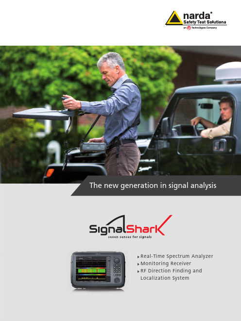
The new generation in signal analysisReal-Time Spectrum AnalyzerMonitoring ReceiverRF Direction Finding andLocalization SystemMore and more devices have to share the available frequency spectrum as aresult of new technologies such as the Internet of things (IoT), machine tomachine (M2M) or car to car (C2C) communications, and the rapidly growing4G/5G mobile networks.It doesn’t matter whether you are making a wideband measurement of entirefrequency ranges, or searching for hidden signals, or needing to reliablydetect very short impulses, or localizing interference signals –SignalSharkgives you all the measurement solutions you need to cope with the increasinglycomplex radio frequency spectrum. Its design and excellent performance makeit ideal for on-site measurements as well as for fully-fledged laboratory use. SignalShark. Seven senses for signalsSignalShark –there’s a reason for the name. Just like its namesake, theSignalShark is an extremely efficient hunter, perfectly designed for its task.Its prey: interference signals. Its success rate: Exceptional. The real-timeanalyzer is a successful hunter, thanks to the interplay of its highly developedseven sensory functions. Seven senses that don’t miss a thing, and that makeit easy for you to identify and track down interferers in real-time./watch?v=pSZdR27j5LQ&t=14s• Frequency range: 8 kHz to 8 GHz• Weight: Approx. 4.1 kg / 9 lbs (with one battery)• Dimensions: 230 × 335 × 85 mm (9.06ʺ× 13.19ʺ× 3.35ʺ)Make it your deviceSignalShark is ready for the future, thanks toits many expansion facilities, and it can beoptimally adapted as needed to the widestvariety of applications.SignalShark – the 40 MHz real-timespectrum analyzerWhether you are in the lab or out in thefield, you will have the right analysis toolin hand with the SignalShark. You will beconvinced by its truly outstanding RF perfor-mance, as well as by its easily understood,application-oriented operating concept.The high real-time bandwidth with very highFFT overlapping ensures that you can reliablycapture even extremely brief and infrequentevents. The unusually fast scan rate results invery short measurement times even if youneed to cover wider frequency bands thanthe real-time bandwidth. Comprehensiveevaluation tools make sure that you canperform current and future measurementand analysis tasks up to laboratory instru-ment standards reliably, simply, and faster.SignalShark – the monitoring receiverThe extremely High Dynamic Range (HDR) ofthe SignalShark ensures that you can reliablydetect even the weakest signals in the pre-sence of very strong signals, and not confusethem with the artifacts of a normal receiver.This is a basic requirement for most tasksin the field of radio monitoring. Alongsidethe real-time spectrum analyzer, there is areceiver for audio demodulation, level mea-surement, and modulation analysis, whichcan be tuned to any frequency and channelbandwidth within the 40 MHz real-timebandwidth. And, if you need even more thanthe analysis tools of the SignalShark, you canprocess the I/Q data from the receiver exter-nally as a real-time stream and store themon internal or external data storage media.SignalShark – the direction findingand localization systemIt is often necessary to locate the positionof a signal transmitter once the signals havebeen detected and analyzed. SignalSharksupports the new Automatic Direction-Finding Antennas (ADFA) from Narda,allowing you to localize the source veryquickly and reliably. In fact, localization ischild’s play, thanks to the integrated mapsand localization firmware. Conveniently,homing-in using an ADFA mounted on amoving vehicle is also supported. Powerful,state of the art algorithms minimize theeffects of false bearings caused by reflectionsoff urban surroundings in real-time. Extre-mely light weight and easy to use manualdirection finding antennas are availablefor ”last mile“ localization.V I D E OVideo display port for external monitor or projector USB 2.0 for keyboard, mouse, printer, etc.fast, convenient measurementBuilt-in loudspeaker gives clear,loud sound reproduction, even in noisy environments/watch?v=0jqrwU_jPcsV I D E OSignalShark is a handy, portable, battery powered measuring device, yet it boasts performance that is otherwise only found in large, heavy laboratory grade equipment. It can be readily used instead of such expensive equipment because of its wide range of connection facilities and measurement functions.SignalShark –the real-time spectrum analyzer• HDR: extremely low noise and distortion, simultaneously • real-time bandwidth: 40 MHz – FFT overlap: 75 % (Fspan > 20 MHz)– FFT overlap: 87.5 % (Fspan ≤20 MHz, RBW ≤400 kHz))– FFT size: up to 16,384• Minimum signal duration for 100 % POI: 3.125 µs at full amplitude accuracy • Minimum detectable signal duration: < 5 ns • Persistence: up to 1.6 million spectrums per second • Spectrogram time resolution: down to 31.25 µs • Spectrogram detectors: up to three at the same time • RBW: 1 Hz - 800 kHz in real-time spectrum mode, 1 Hz - 6.25 MHz in scan spectrum mode• Filters conforming to CISPR and MIL for EMC measurements • Scan speed: Scan rate up to 50 GHz/s • Detectors: +Pk, RMS, Avg, -Pk, Sample• Markers: 8, additional noise power density and channel power function •Peak table: shows up to 50 highest spectral peaksReliable detection of extremely short and rare events in a 40 MHz real-time bandwidthA real-time analyzer calculates the spectrum by applying the FFT on overlapping time segments of the underlying I/Q data within its real-time bandwidth. The real-time band-width is only one of the key parameters for a real-time analyzer. The probability of inter-cept, POI, is easily just as important. This parameter describes the minimum time that the signal must be present for it to be always detected without any reduction in level. This time is affected by the maximum resolution bandwidth RBW and the FFT overlap. The SignalShark is a match for established laboratory analyzers with its minimum duration of 3.125 µsec for 100 %POI and full amplitude accuracy. The mini-mum detectable signal duration is < 5 nsec.SignalShark accomplishes this by a large signal immunity in combination with a very low intrinsic noise as well as a high FFT overlap and its large resolution bandwidth.That is outstanding for a hand-held analyzer. To accomplish this, SignalShark generally operates with an 87.5 % overlap, which is again outstanding for a hand-held analyzer.This means that even the shortest impulses are detected and the full signal to noise ratio is maintained for longer signals.Spectrogram shows more details than everWith SignalShark, you can use up to three detectors at the same time for the Spectrogram view. This makes it possible for you to easily visualize impulse inter-ference on broadcast signals and get much more information from the spectrogram. The extraordinarily fine time resolution of 31.25 µs means that you can completely reveal the time signatures of many signals.With the I/Q Analyzer option, you can resolve the spectrogram even more, to less than 200 ns.Persistence ViewA color display of the spectrum shows how often the displayed levels have occurred. This enables you to detect signals that would be masked by stronger signals in a normal spectrum view.=SignalShark is not just a very powerful real-time spectrum analyzer. It is also the ideal monitoring receiver, thanks to its near ITU-ideal spectrum monitoring dynamic capabilities, second receiver path and demodulators.SignalShark –the monitoring receiver• HDR: extremely low noise and distortion, simultaneously • CBW: 25 Hz - 40 MHz (Parks-McClellan, α= 0.16)• Filters for EMC measurements: CISPR, MIL • Detectors: +Pk, RMS, Avg, -Pk, Sample• EMC detectors: CPk, CRMS, CAvg (compliant with CISPR)• Level units: dBm, dB µV, dB(µV/m) …• Level uncertainty: < ±2dB • AFC• Audio demodulators: CW, AM, Pulse, FM, PM, LSB, USB, ISB, I/Q • AGC & squelch for audio demodulators • Modulation measurements: AM, FM, PM • I/Q streaming: Vita 49 (sample rate ≤25,6 MHz)• Remote control protocol: SCPIThe benefit of HDRThe extremely high dynamic range (HDR) of the SignalShark ensures that you can reliably detect even the weakest signals in the presence of very strong signals. The SignalShark’s pre-selector allows it to suppress frequencies that would other-wise interfere with the measurement. The excellent dynamic range of the SignalShark is the result of the ideal combination of the displayed averaged noise level (DANL)with the so-called large-signal immunity parameters, i.e. the second and third order intermodulation intercept points (IP 2and IP 3).It is important that these three factors are always specified for the same device setting (e.g. no attenuation, no pre-amplifier), as they vary considerably according to the setting.DDC 2, the additional receiver pathThe tuning frequency and the channel band-width of an additional receiver path, DDC 2,can be set independently from the real-time spectrum analyzer path, DDC 1, within the real-time bandwidth of the SignalShark. The I/Q data can be streamed to external devices in real-time, or they can be processed by the SignalShark itself for level measurements,audio demodulation, and modulation measurements. The very steep cutoffchannel filters capture 100 % of the signal in the selected channel without any degra-dation while completely suppressing the adjacent channels.CISPR compliant EMC detectors now also available for on-site applications The facility for selecting all the filters and detectors necessary for CISPR or MIL com-pliant EMC measurements is also available for the receiver as well as for the spectrum. If an interferer is detected, you can now decide on the spot whether or not the device needs to be taken out of service because of violating EMC regulations.EQDDC 1Overlap BufferFFT DetectorsPersist.Persistence StreamSpectrum StreamADC DataDDC 2DetectorsDetectorsI/Q BufferTrigger UnitDemodulatorsAGCLevel StreamDem. Det.StreamDem. Audio StreamAM & FM StreamI/Q StreamI 2+Q2I 2+Q2PATH 1PATH 2The block circuit diagram shows the two, independent digital down converters (DDC). These make it possible e.g. to observe the spectrum of the signal spectrum and demodulate it at the same time independently within the real-time bandwidth.Automatic Direction Finding Antenna ADFA 1 + 2Narda offers a large number of automatic and directional antennas for the SignalShark. Their unique characteristics combined with the SignalShark makes them unbeatable.Automatic Direction Finding Antenna ADFA 1The frequency range of ADFA 1 makes it particularly suitable for localizing interferers,e.g. in mobile communications networks:Frequency range: 200 MHz - 2.7 GHz Nine dipoles arranged on a 380 mm diameter circle for DFA central monopole is used as a reference element for DF or as an omnidirectional monitoring antennaBuilt-in phase shifter and switch matrix Direction finding method: correlative interferometerBearing uncertainty: 1° RMS (typ.)Built-in electronic compassBuilt-in GNSS receiver with antenna and PPS outputDiameter: 480 mmAutomatic Direction Finding Antenna ADFA 2 (available 2019)This ADFA is suitable for a wide range of localization tasks due to its wide frequency range:Frequency range: (500 kHz) 10 MHz -8 GHz Two crossed coils for DF at low frequencies Nine dipoles arranged on a 380 mm dia-meter circle for DF at medium frequencies Nine monopoles arranged on a 125 mm diameter circle for DF at high frequencies A central monopole is used as a reference element for DF or as an omnidirectional monitoring antennaBuilt-in phase shifter and switch matrix Direction finding method: Watson-Watt or correlative interferometerBearing uncertainty (10 MHz - 200 MHz): 2° RMS (typ.)Bearing uncertainty (200 MHz - 8 GHz): 1° RMS (typ.)Built-in electronic compassBuilt-in GNSS receiver with antenna and PPS output Diameter: 480 mm Automatic Direction Finding Antenna ADFA accessoriesConnecting cable, length 5 m or 15 m,low lossTripod including mounting accessories Mounting kit for magnetic attachment to a vehicle roofMounting kit for mast attachmentAfter you have localized the signal by SignalShark and ADFA using the car, you will need for last mile or to enter a building Narda’s handy, feather-light directional antennas and active antenna handle. They are the ideal choice in this situation. The antenna handle does more than just hold the antenna. Among other features, it has a built-in operating button that allows you to perform the main steps during manual direction finding, making the combination unbeatable.and take bearings on very weak or distant signals. The preamplifier gain is taken into account automatically when you make field strength or level measurements.The integrated operating button lets you make the main steps in the manual direction finding process.The following antennas to fit the antenna handle are available:• Loop Antenna: 9 kHz - 30 MHz• Directional Antenna 1: 20 MHz - 250 MHz • Directional Antenna 2: 200 MHz - 500 MHz • Directional Antenna 3: 400 MHz - 8 GHz A plug-in adapter with male N connector allows you to take advantage of the features of the handle even when you are using third-party antennas or external filters.Directional antenna 3400 MHz - 8 GHz350 g / 0.77 lbsDirectional antenna 1 20 MHz - 250 MHz 400 g / 0.88 lbs Loop antenna 9 kHz - 30 MHz 380 g / 0.84 lbs Directional antenna 2 200 MHz - 500 MHz 300 g / 0.66 lbs Active antenna handle with integrated compass and preamplifier 9 kHz - 8 GHz 470 g / 1.04 lbsAdapter,male N connectorN Antenna Elements0°90°180°270°Element SwitchReference Elementn1Quadrature Phase Shifter(Smart Antenna)+The Narda antenna handle and directional antennas are extremely light, making for fatigue-free signal searches.The convenient plug-in system allows you to change antennas very quickly.SignalShark recognizes the antenna and applies the appropriate antenna factors for field strength measurements automatically.SignalShark receives the azimuth,elevation and polarization of the antenna from the 3D electronic compass built into the handle, so manual direction finding could hardly be simpler.The preamplifier built into the handle is activated and deactivated bySignalShark, so you can further reduce SignalShark’s low noise figure to detectYou will often need to locate the position of a signal transmitter once thesignals have been detected or analyzed. SignalShark combined with Narda’snew automatic direction finding antennas (ADFA) and the very powerfulmap and localization firmware provides reliable bearings in the twinklingof an eye. The bearing results are processed by the SignalShark withoutneeding an external PC. Reliable localization of transmitters has not beenpossible before with so few hardware components.Transmitter localizationSignalShark simplifies transmitter localizationby autonomously evaluating all the availablebearing results and plotting them on a map,using a statistical distribution of bearinglines. The result is a so-called “heat map”,on which the possible location of the trans-mitter is plotted and color-coded accordingto probability. SignalShark also draws anellipse on the map centered on the estima-ted position of the transmitter and indicatingthe area where the transmitter has a 95 %probability of being located. The algorithmused by SignalShark to calculate the positionof an emitter is extremely powerful. It candetermine the position of the emitter bycontinuous direction finding when movingaround in a vehicle, even in a complexenvironment such as an inner-city area.The calculation is continuous inreal-time, so you can viewthe changing heat mapon the screen of theSignalShark andFast automatic direction findingSignalShark supports the new automaticdirection finding antennas (ADFA) fromNarda, which let you take a completebearing cycle in as little as 1.2 ms.The omnidirectional channel power and thespectrum are also measured during a bearingcycle, so you can monitor changes in thesignal level or spectrum concurrently withthe bearings. The AFDAs use differentantenna arrays, depending on the frequencyrange. At low frequencies, a pair of crossedcoils are used for the Watson-Watt methodof direction finding. At medium and highfrequencies, a circular array of nine dipolesor monopoles is used for the correlativeinterferometer direction finding method.SignalShark –The RF direction finding and localization system• Frequency range ADFA 1: 200 MHz - 2.7 GHz• Frequency range ADFA 2: 10 MHz - 8 GHz• Azimuth and elevation bearings• DF quality index• Complete bearing cycle: down to 1.2 ms• Omnidirectional level and spectrum during DF process• Uses OpenStreetMaps, other map formats can be imported• Easy to use, powerful map and localization software• The map and localization software runs on the handheldunit itselfThe SignalShark is a very powerful platform that Narda is continuously expanding. Options that will be available for delivery in 2019 are described below. Only the firmware of the SignalShark will be used to realize these options, which will be capable of on-site activation.High time resolution spectrogram HTRSalso available in the spectrum pathIn real-time spectrum mode, the ring buffer ofthe SignalShark records the I/Q data from thereal-time spectrum path rather than from thereceiver I/Q data. If you or a trigger eventhalts the real-time analyzer, the last up to200 million I/Q samples of the monitoredfrequency range are available. This correspondsto a timespan of at least 4 s, so you can zoomin on the spectrogram with a resolution ofbetter than 200 ns when the analyzer is halted.The FFT overlap can be up to 93.75 %, and nodetectors are needed that could reduce thetime resolution. You can even subsequentlyalter the RBW. The persistence view also adjustsso that it exactly summarizes the spectrumsin the time period covered by the zoomedsegment. This ensures that all the time orspectral details in the I/Q data can be madevisible. You can of course also save the I/Qdata of the zoomed segment.DF SpectrumThe SignalShark can find the directions ofseveral transmitters simultaneously in DFspectrum evaluation mode. This mode offersa persistence spectrum and a spectrogramof the azimuth in addition to the usual levelspectrum and spectrogram view. You canalso monitor frequency ranges that arewider than the real-time bandwidth of theSignalShark. You can distinguish betweendifferent transmitters much more easilythan before by means of DF spectrum mode,because the SignalShark shows you thedirection of incidence as well as the levelof each frequency bin.SignalShark I/Q analyzerSignalShark has a ring buffer for up to 200 million I/Q samples. The receiver I/Q data are normally written continuouslyto the ring buffer. The recording can be stopped by a trigger event. The recorded I/Q data are then transferred to the CPU of the SignalShark, where they are further processed.The following trigger sources are available: Frequency mask triggerReceiver levelExternal trigger sourceTimestampUser inputFree runThe following I/Q data views are available: I and Q versus timeMagnitude versus time (Zero-span) Vector diagramHigh time resolution spectrogram Persistence You can of course also save the I/Q data as adata set, and you can even stream the datadirectly to permanent storage media in orderto make very long recordings of the I/Q data.You can then replay such long-term recor-dings using the integrated I/Q analyzer, orprocess them externally.2 x 10 MHz LTE signal recorded in a HTRS. Time resolution1 µs. The extremely high time resolution renders the signaltransparent at low traffic levels (right), so you can spotpossible interference within the frame structure.More Information about technical details andaccessories like transport case and car chargerunit can be found in the SignalShark data sheet./en/signalsharkNarda is a leading supplier …N S T S 06/18 E 0333A T e c h n i c a l a d v an c e s , e r r o r s a n d o m i s s i o n s e x c l u d e d .© N a r d a S a f e t y T e s t S o l u t i o n s 2014. ® T h e n a m e a n d l o g o a r e t h e r e g i s t e r e d t r a d e m a r k s o f N a r d a S a f e t y T e s t S o l u t i o n s G m b H a n d L 3 C o m m u n i c a t i o n s H o l d i n g s , I n c .—T r a d e n a m e s a r e t h e t r a d e m a r k s o f t h e i r o w n e r s .r o e n e r -d e s i g n .d eNarda Safety Test Solutions 435 Moreland RoadHauppauge, NY11788, USA Phone +1 631 231-1700Fax +1 631 231-1711**************************… of measuring equipment in the RF test and measurement, EMF safety and EMC sectors. The RF test and measurement sector covers analyzers and instruments for measuring andidentifying radio sources. The EMF safety product spectrum includes wideband and frequency-selective measuring devices, and monitors for wide area coverage or which can be worn on the body for personal safety. The EMC sector offers instruments for determining the electro-magnetic compatibility of devices under the PMM brand. The range of services includes servicing, calibration, accredited calibration, and continuous training programs.Narda Safety Test Solutions GmbH Sandwiesenstraße 772793 Pfullingen, Germany Tel. +49 7121 97 32 0Fax +49 7121 97 32 790********************* /en/signalshark。
TM影像的计算机屏幕解译和荒漠化监测-林业科学研究

1998-04-29收稿。
张玉贵研究员,刘华(中国林业科学研究院资源信息研究所 北京 100091);F .R .Beern aert (联合国粮农组织土地分类顾问)。
*本文是国家“八五”攻关专题“‘三北’防护林体系和植被动态监测及信息系统研究”和GC P /C PR /009/BEL 国际合作项目的部分内容。
T M 影像的计算机屏幕解译和荒漠化监测*张玉贵 F.R.Beernaert 刘 华 摘要 以覆盖科尔沁沙地13个旗县的6景T M 影像为例,简介了以计算机屏幕解译这种技术路线制作卫星影像分类图的过程,论述了卫星遥感技术监测荒漠化土地变化和作出环境发展趋势评估的潜力。
指出对待盐渍化和沙化这两个问题,对不同区域应各有侧重,最后介绍了联合国粮农组织(FA O )的土地分类原则,用土地单元、土地利用类型及附加特性注记地类的方法。
关键词 荒漠监测 遥感 环境评价 荒漠化威胁着全人类的生存环境。
在中国,由于人为因素,除个别地区表现出生态环境好转以外,荒漠化日趋严重是总的趋势。
监测、控制和治理荒漠化是一个社会问题,需要各级政府和受益区群众共同协作,才能解决。
遥感技术是一种有效监测荒漠化的手段。
卫星遥感影像是对地物本身特性的客观反映,但缺少抽象地理要素,需要加入地理信息以确定地理位置和方向,这就形成了影像地图。
经过现地调查、分析、解译并勾绘出不同地物的界线,并保留原影像特征,便生成卫星影像分类地图。
本文主要介绍T M 影像监测荒漠化的潜力以及卫星影像地图及分类地图的技术要点。
1 T M 影像处理方法 荒漠化土地的计算机屏幕解译以及卫星影像地图及卫星影像分类图的制作,主要是在微机上用Photoshop 软件完成,但原始影像需做预处理。
1.1 数据资料及预处理购置内蒙古科尔沁沙地1996年的T M 影像数据6景,其轨道号为122/29、122/30、121/29、121/30、120/29、120/30。
landmark分频处理工作流程

• 二、Animation(制作)
• 通过启动制作调谐体,观察并最终决定带宽;也就决定这相干的地质信息能否被观 测到。
• 三、Selection(选择)
• 选择一对相对独立的频率体成像显示当前的目的层地质地形。
• 如果在这个流程中没有相干的地质信息被观测到,那么接着,SpecDecomp工具就 不能被用来加深你对目的层层位的解释/理解。如果这个流程KO了,你就能够最优化你 的调谐参数,作进一步的详细分析。
• 6.设置基准时间为1025ms。 • 7.选择最大时窗长度,使用MB3 在时窗长度输入栏中。 •注意你可以使用MB3在输入各项,可以得到可用输入值的列表。 • 8.最大频率改为250. • 9.将余弦梯度给定为20%。
• 10.为Workflow_2_1设置数据体前缀. • 11.选择Output Horizons... • 12.选择Autocreate (自动生成) 如下层位。
•7.默认其他参数并选择需计算数据体。
•计算会给予你5分多钟的休 息时间,具体在于你机器的 性能。如果你的机器不是那 么快,你可以去小憩一会。
•计算每道DFT
•8.确定计算完成
•过滤、标准、归 类频率切片
•制作:
• 现在你预备去启动地 震波剖面,选择一些分立的 频率对目的层段地质地形成 像。
•2.打开SD_wf_1-0-1.t.w3s 时域。
•凭直觉你能看到已调谐地层的 高振幅部分,得注意在此图上 色标是反转的。
•是不是FirstPeak_Frep 层看 来就像是沿着首峰的轨迹而来 的?移动光标沿着并观看显示 图底部振幅值的输出,你会看 到一些振幅的峰值在计算出的 FirstPeak_Frep 层之上。
• 在具体处理之前,你需作到所选择的层必须经过内插而且要贯穿所有断层。频谱分 析通常能使断层更加明了,这使你能重新去认识这些断层,在频谱成像上。如果你的层 位具有相对高的信噪比和稳定的地震波同相轴, 还得考虑对数据作剩余静校正。 这一步 将清除许多由于工作站上自动追踪的同相轴所引起的跳跃现象。你也可以通过简单的圆 滑地层来处理。频谱分析前的这步会敏锐地提高成像质量。这种提高能使你恰好得到地 质信息的一个重要部分。
海岸地形测量技术科普:机载LiDAR测量技术的应用

海岸地形测量技术科普:机载LiDAR测量技术的应用海岸地形测量是海洋测绘的重要组成部分,主要包括三部分内容:海岸线;海岸线以上一定范围内的航行方位物、道路、河流、沟渠,居民地,植被、土质等;海岸线以下干出滩、明礁、岛屿以及码头,海堤、灯塔、渔堰等重要地物。
由于海道测量规范对海岸线,干出滩性质与高程,航行方位物等要素信息的测量精度要求较高,所以,传统海岸地形测量主要采用数字全站仪和 GPS RTK 等人工实地精确测量方法。
随着机载LiDAR技术及其应用的快速发展,使海岸地形测量的技术创新成为可能。
检测具有国家认可的测绘资质,拥有多名专业级海洋测绘高级工程师、注册测绘师。
我们将利用自身专业的技术、丰富的经验和完善的设备,为客户专业化的海岸地形测量服务。
海岸线机载LiDAR 测量按照《海道测量规范》要求,海岸线应实测,即根据海岸的植物边线、土壤和植被的颜色、湿度、硬度以及流木,水草、贝壳等冲积物人工实地测定,并按性质分为岩石岸、磊石岸、砾质岸、沙质岸、陡岸、岩石陡岸,加固岸,垄岸,详细测注高程,高程测量中误差不大于0.2m ,陡岸、堤岸均须注记比高等。
《海道测量规范》要求海岸线实测。
20世纪90年代受测量技术水平的限制,但是目前基于航空摄影测量和激光雷达扫描测量的地形图测绘技术发展很快,测图比例尺普遍达到1:2000,影像分辨率高于0.2m ,最高可达0. 05m,通过影像解译提取海岸线已成为现实,加之高精度、高密度的激光点云数据,准确勾画出海岸线等高特征,确保海岸线识别定位信息准确可靠,同时机载LiDAR了海岸线高程注记和地物比高信息,再结合外业调绘,实现海岸线精细分类。
单一摄影测量无法满足海岸线高程测量精度和精细分类要求,而机载LiDAR测量包含摄影测量和激光点云测量两部分功能,再结合外业调绘技术,使机载 LiDAR成为海岸线测量的有效手段。
滩涂机载LiDAR测量滩涂测量包括海岸线以下干出滩、明礁、岛屿等,以及码头,海堤,灯塔、渔堰等重要地物,要求高程测量中误差不大于0. 2m。
纳达场域人手:全功能电磁场仪说明书

DatasheetNarda FieldManNarda FieldMan ®All-in-one electromagnetic field meter ranging from 0 Hz to 90 GHzThe Narda FieldMan performs highly accurate measure-ments of non-ionizing high-frequency radiation and low-frequency fields. Equipped with digital probes for measuring electric or magnetic field strengths, it covers the range from static and low-frequency fields in medical and industrial applications to mobile radio frequencies and millimeter waves. Flat frequency response probes (“flat probes”), as well as so-called shaped probes that evaluate the field strength on the basis of a human safety standard are available. Probes with built-in FFT analysis enable spectral measurements along with time domain analyses up to frequencies of 400 kHz. All probes have a digital interface that transmits the measurement data to the basic device in a fail-safe manner. This eliminates the need to calibrate the basic unit.›Non-directional measurement using isotropic probes for applications in the frequency range 0 Hz (DC) to 90 GHz›Large sunlight readable color display 5” diagonal with 1280x720 HD resolution›Digital probe interface for broadband and selective probes – no more meter calibration›Powerful time and frequency domain analysis for low frequency fields up to 400 kHz including Weighted Peak measurements›WiFi/Bluetooth interface for remote operation via smartphone app (Option)›Built-in GPS receiver and rangefinder for easy location determination (Option)›Fast data transmission ›optical interface ›Ethernet ›USB-CApplicationsThe Narda FieldMan is used to make precision measurements to establish human safety, particularly in workplace environments where high electric or magnetic field strengths are likely to occur. An essential task is to demonstrate compliance with generalsafety regulations, such as FCC, IEEE, ICNIRP or EMF Directive 2013/35/EU. Examples of measurement environments are:›Radiocommunication base stations (e.g. IEC / EN 62232)›Broadcasting systems (e.g. IEC 62577)›Radar and satellite communications systems ›Induction heating and melting (e.g. EN 50519)›Household appliances (e.g. IEC / EN 62233)›Electric welding equipment (e.g. IEC / EN 62822)›Railroad operations (e.g. EN 50500)›Automotive operations (e.g. IEC 62764)›Energy supply systems (e.g. IEC / EN 62110)›Electrical medical devices (e.g. IEC / EN 60601)›TEM cells and absorber chambers to demonstrate electromagnetic compatibility (EMC)Digital ProbesA large number of isotropic field probes are available for theFieldMan. All of them transmit their information and measurement data as a digital signal to the FieldMan, either via an electrical USB interface or via an optical COM interface. In this way,interference is significantly reduced compared to high-resistance analog interfaces. The specially developed screw connectors and electrical contacts are extremely robust and resilient.The probes are automatically recognized after connection to the FieldMan. Sensors inside the probe record the temperature of the measuring location and transmit it to the FieldMan display. In addition to the automatic offset correction, the temperature measurement is also used to compensate for the typicaltemperature dependency of the sensor diodes. The advantages are uninterrupted measurements without zero adjustment and higher measurement accuracy over wide temperature ranges. An automatic self-test function can even detect possible errors in the sensor system, which means that additional checking with a test generator is superfluous. Only the digital probes arecalibrated. You can continue to use your FieldMan during this time.There are probes for many different applications with theappropriate frequency and level ranges. The following table gives an overview of common areas of application.Frequency rangeDC up to1 kHzUp to400 kHzUp to400 kHz Up to 30 MHz Up to 1 GHz Up to 6 GHz Up to 40 GHz Up to 90 GHz Up to 50 GHz Field type, magnetic (H) or electric (E)H E+HHHHEEEE ShapedProbe modelsHP-01EHP-50F/G BFD-400-1 (100 cm 2) BFD-400-3 (3 cm 2) HFD-3061 HFD-0191 EFD-0391 EFD-0392 EFD-0691 EFD-0692 EFD-1891 EFD-4091 EFD-5091 EFD-6091EFD-9091EAD-5091EBD-5091ECD-5091EDD-50915G mobile radio / telecommunications Broadcast radio / TVSatellite communications RadarIndustry: Heating and temperingIndustry: Plastics weldingIndustry: Semiconductor productionMedicine: Diathermy, hyperthermyLeak locationHousehold appliances Electric welding equipmentRailroad operationsAutomotive operationsEnergy supply systems Electric medical devicesAccredited calibration includedProbe interfaceOptical connectionDigital probe interfaceFig. 1. Areas of application and suitable probe modelsUse and benefitDuring the development of the FieldMan, special attention was paid to achieving simple, well-structured and fluid operation. The arrangement of many display elements known from smartphones, the self-explanatory symbols and the FieldMan processes, which are perfectly tailored to the measurement tasks, offer maximum ease of use. The large, anti-glare HD color display shows the measured values numerically and graphically with all important additional information in a clear form and is easy to read even in bright sunlight. From simple broadband measurements to sophisticated time signal recording in real time or spectral frequency analysis of low-frequency fields, you have the right operating modes at your disposal.Measurement results can be commented on by text or voice and can be saved as a screen copy at the push of a button. Built-in sensors record the current environmental conditions as well as the position data and automatically add them to the measurement result. The built-in distance meter (option) shows you the measuring height above the ground, which makes the exact positioning of the measuring device much easier. For a better overview, the measurement results can be assigned to freely definable projects, which is particularly helpful when the measurement locations change frequently. If you want todocument your measurement results with photos and videos, the FieldMan smartphone app will help you. For example, the app wirelessly transfers media files created with the smartphone to the project directory on the FieldMan SD memory card. A newly developed, extremely powerful PC software "Narda-TSX" is available for documenting the measurement results, media and other information. It is Narda's new software platform for device configuration, measurement data evaluation and documentation, which in addition to the FieldMan will also support other Narda products in the future.Fig. 2. FieldMan display and controlsFig. 3. The FieldMan is supplied with a robust transport caseProbe connectionBrightness sensor LoudspeakerMicrophone, humidity sensor Status bar Probe information Measurement informationMeasurement isotropic Measurement single axes Statistical values Interface panelMeasurement graphic: Time curve, spectrum or bar graph Softkey symbolsSoftkeys Save key Back key Navigation keyStatus LEDDefinitions and ConditionsConditionsUnless otherwise noted, specifications apply after 30 minutes warm-up time within the specified environmental conditions. The product is within the recommended calibration cycle.Specifications with limitsThese describe product performance for the given parameter covered by warranty. Specifications with limits (shown as <, ≤, >, ≥, ±, max., min.) apply under the given conditions for the product and are tested during production, considering measurement uncertainty.Specifications without limitsThese describe product performance for the given parameter covered by warranty. Specifications without limits represent values with negligible deviations, which are ensured by design (e.g. dimensions or resolution of a setting parameter). Typical values (typ.)These characterize product performance for the given parameter that is not covered by warranty. When stated as a range or as a limit (shown as <, ≤, >, ≥, ±, max., min.), they represent the performance met by approximately 80% of the instruments. Otherwise, they represent the mean value. The measurement uncertainty is not taken into account. Nominal values (nom.)These characterize expected product performance for the given parameter that is not covered by warranty. Nominal values are verified during product development but are not tested during production. UncertaintiesThese characterize the dispersion of the values attributed to the measurands with an estimated confidence level of approximately 95%. Uncertainty is stated as the standard uncertainty multiplied by the coverage factor k=2 based on the normal distribution. The evaluation has been carried out in accordance with the rules of the “Guide to the Expression of Uncertainty in Measurement” (GUM).Specifications MetricsElectric and magnetic fieldsMeasurement control and result display for the following probes and analyzers.Frequency range and level range depending on the probe/ analyzer. Broadband probes 100 kHz to 90 GHz (see list of digital broadband probes)Selective probes 1 Hz to 400 kHz, B-field (see list of digital selective probes)Probe model EHP-50F/G 1 Hz to 400 kHz, E-field and B-field (FFT-Analyzer, see separate datasheet)Probe model HP-01 0 Hz to 1 kHz, B-field (Magnetometer/ FFT-Analyzer, see separate datasheet)Electric field units V/m, mW/cm2, W/m2, % of standard (depending on the connected probe)Magnetic field units A/m, Tesla, Gauss, mW/cm2, W/m2, % of standard (depending on the connected probe)Temperature 1Logging of the ambient temperature at the time of measurement (-40 °C to +85 °C) in °C or °F Humidity 1Logging of the ambient relative humidity at the time of measurement (0% to 100% RH)Air pressure Logging of the ambient air pressure at the time of measurement (300 to 1100 hPa)Distance (Option) An ultrasonic rangefinder on the bottom side measures the distance to ground or to an object (0.25 m to 4 m) in m, ft, in or yd. Coverage ratio ≈ Distance / 4.Geolocation (Option) Built-in GNSS receiver for determining latitude, longitude and altitude (MSL).72 channels with the support of GNSS systems (GPS / QZSS, Galileo, GLONASS, BeiDou) and the SBAS extension system (WAAS, EGNOS, MSAS, GAGAN).Position accuracy: Autonomous 2.5 m CEP.DisplayDisplay type Sunlight readable 5” color TFT-LCD anti-glare display (HD 1280 x 720 pixels) Brightness Manual control or automatic control via brightness sensorOperating languages Largely language-independent measurement control via symbols.Menu languages: English, German, more are planned.1 The permissible operating range of the device and probe must not be exceeded. The temperature sensor is located in the probe.Operating ModesMode description Field Strength Broadband field measurements. Numerical results with time curve or bar graph display.Spatial Average Procedure for spatial averaging of broadband measurements over several measurement positions. Timer Logging Time-controlled broadband measurement of the field strength in a definable period.Spectrum FFT analysis with spectrum display, marker evaluation and display of the broadband level. Shaped Time Domain Time domain assessment (WPM, WRM) with digital filtering related to a selected safety limit. Scope Triggered measurement of the field curve over time with pretrigger feature.Available modes Broadband ProbesDigital Interface100 kHz to 90 GHzSelective ProbesDigital Interface1 Hz to 400 kHzModel EHP-50F/GOptical Interface1 Hz to 400 kHzModel HP-01Optical InterfaceDC to 1 kHzField Strength ☑☑☑☑Spatial Average ☑☑☑☑Timer Logging ☑☑☑☑Spectrum ☑☑☑Shaped Time Domain ☑☑Scope ☑FeaturesProbe features Recognition Probes are automatically recognized after being plugged in.Operating principle Measurement signals are sampled and processed inside the probe and provided as digital values. Offset compensation Automatic offset compensation enables gapless RF measurements without zero adjustment.Self-test Functional test including the sensor function of each measuring axis for digital interface probes.Signal detection RMS detection, Peak detection for WPM measurementsand selectable detection RMS/Peak with BDF-400 probes.Numerical display Total field (isotropic) and field components X, Y, Z (for probes up to 18 GHz).Result types Field Strength Actual, Max, Min, Avg (average) and Max Avg Spectrum Actual or Max or AvgShaped Time Domain Actual, Max and MinScope Actual, Max and marker for dB/dtAverage mode Moving average over time of the square values of the field strength.Averaging time Field Strength,Timer Logging 1 s, 3 s, 10 s, 30 s, 1 min, 3 min, 6 min, 10 min, 30 min, 1 h, 6 h, or 24 h Spectrum 4, 8, 16, 32 or 64 number of averagesGraphical display with marker function Field Strength Actual and Avg trace vs. time, time span selectable from 48 s to 24 hours.Spatial Average Bar graph of results for each measurement position (≤100) and the spatial average line. Timer Logging Timeline during measurement, results as a graph vs. time after measurement.Spectrum Frequency spectrum and selectable limit line. All axes are measured, one can be displayed. Shaped Time Domain Exposure index (WPM or WRM) in % vs. time, time span selectable from 4 min to 24 h. Scope Sign-based recorded signal with 25 % pretrigger. Recording time selectable from 1 ms to 30 s.Screenshots Manually initiated screenshot or automatically when saving a measurement result.Comments Voice and/or text comments can be assigned to a measurement result.Alarm Alarm sound and alarm message when an adjustable field strength is exceeded.Audible field indicator Acoustic hotspot search with field strength-dependent audio frequency (available for RF-probes).Scheduled measurements Mode Timer Logging with automatic wake-up and shutdown after measurement. Start time pre-selection: up to 24 h or immediate startTimer duration: up to 100 hStorage interval: 1s to 6 min (in 11 steps, up to 32000 intervals)Correction factors Post-processing for broadband probes to increase the accuracy at a known field frequency(direct frequency entry, interpolation between calibration points)Probe interface Digital probe interface for direct connection or via the optional extension cable.Optical port Serial, full duplex, ≥ 1 Mbit/s, to connect the Field Analyzer EHP-50F/G, the Magnetometer HP-01or the Digital Probe Repeater. Recommended interface for PC controlled measurements.USB 2.0 USB-C connection for battery charging, remote control and data transfer.Ethernet Gigabit Ethernet LAN connectivity for remote control and data transfer.Bluetooth (Option) BT 4.0 for remote control via smartphone app (Android).WiFi (Option) WLAN connectivity for remote control and data transfer.AUX MMCX connector, reserved for future use.Result StorageStorage triggers Manual (by keypress) or scheduled (Timer Logging Mode).Storage medium Removable micro SD card for storing measurement data, setups and comments.Storage capacity Up to 128 GB.16 GB micro SD card included.Screenshots Screenshots can be saved for documentation as PNG files.Voice recorder Voice comments can be added to measurement results (recording and playback).Text editor Text comments can be added to measurement results (integrated virtual keyboard).Photos / videos (WiFi/BT Option) Photos and videos from a smartphone can be transferred to the device using the FieldMan app.Printouts (WiFi/BT Option) Saved measurement results can be printed locally by using the FieldMan Android app for on-sitedocumentation (requires a compatible wireless printer).General SpecificationsRecommended calibration interval Calibration of the basic unit is not required. Only the probes are calibrated.Power supply internal Li-Ion rechargeable battery pack, included and replaceable external USB-C PD (maximum 12 V / 3A, compatible with BC1.2 and QC 3.0)Operating time (nom.) 16 hours (with broadband probes and analyzers)Charging time (nom.) 4 hours (80% charged in 2½ h)RF Immunity 200 V/m (100 kHz to 60 GHz); can be below the permissible measuring range of a probe. Operation in static magnetic fields ≤ 30 mT (to avoid high force on the device)Dimensions (H x W x D) 51 mm x 93 mm x 312 mm without probeWeight 695 g (without probe)Country of origin GermanyEnvironmental ConditionsRange of application Suitable for outdoor use and an operating altitude of up to 5000 mOperating temperature -20 °C to +50 °C during normal operation with battery0 °C to 40 °C during the charging process with an external chargerHumidity < 29 g/m³ (< 93 % RH at +30 °C), non-condensingIngress protection IP54 (probe screwed on, protective flap closed, stand folded in)Climatic conditions Storage 1K4 (IEC 60721-3) extended to -30 °C to +70 °C (battery removed)1K3 (IEC 60721-3) extended to -20 °C to +50 °C (battery inserted) Transport 2K3 (IEC 60721-3) extended to -30 °C to +70° COperating 7K2 (IEC 60721-3) extended to -20 °C to +50 °CMechanical conditions Storage 1M3 (IEC 60721-3) Transport 2M3 (IEC 60721-3) Operating 7M3 (IEC 60721-3)EMC European Union Complies with Directive 2014/53/EU, EN 301489-1, EN 301489-17 and EN 61326 -1 Immunity IEC/EN: 61000-4-2, 61000-4-3, 61000-4-4, 61000-4-5, 61000-4-6, 61000-4-8, 61000-4-11 Emissions IEC/EN: 61000-3-2, 61000-3-3, IEC/EN 55011 (CISPR 11) Class BSafety Complies with European Low Voltage Directive 2014/35/EU and IEC/EN 61010-1 Material Complies with European RoHS Directive 2011/65/EU and (EU)2015/863ORDERING INFORMATIONInstrument SetsDescription Part number FieldMan Basic Set-Probes are not included –Includes:›FieldMan Basic Unit›Hard Case for FieldMan and up to 5 Probes ›Power Supply USB-C PD, AU/EU/UK/US Plugs ›Cable, 2x USB-C(M), 3 A, 2 m›Shoulder Strap, 1 m ›Marking Rings for FieldMan Probes›Quick Start Guide›Safety Instructions›USB Stick: Manuals and Documents›Software Narda-TSX (free download)2460/101Digital Broadband ProbesDescription Part number Probe HFD-3061, H-Field, 300 kHz–30 MHz 2462/05 Probe HFD-0191, H-Field, 27 MHz–1 GHz 2462/06 Probe EFD-0391, E-Field, 100 kHz–3 GHz 2462/01 Probe EFD-0392, E-Field, High Power, 100 kHz–3 GHz 2462/12 Probe EFD-0691, E-Field, 100 kHz–6 GHz 2462/14 Probe EFD-0692, E-Field, 600 MHz–6 GHz 2462/20 Probe EFD-1891, E-Field, up to 18 GHz2462/02 Probe EFD-4091, E-Field, up to 40 GHz 2462/19 Probe EFD-5091, E-Field, 300 MHz–50 GHz, Thermocouple2462/03 Probe EFD-6091, E-Field, 100 MHz–60 GHz2462/17 Probe EFD-9091, E-Field, 100 MHz–90 GHz2462/18 Probe EAD-5091, FCC 1997 Controlled, Shaped, 300 kHz–50 GHz, E-Field 2462/07 Probe EBD-5091, IEEE 2019 Restricted, Shaped, 3 MHz–50 GHz, E-Field 2462/21 Probe ECD-5091, SC 6 2015 Controlled, Shaped, 300 kHz–50 GHz, E-Field 2462/16 Probe EDD-5091, ICNIRP 2020 Occ, Shaped, 300 kHz–50 GHz, E-Field 2462/22 Note: Separate data sheets are available for the probesDigital Selective ProbesDescription Part number Probe BFD-400-1, B-Field, 100 cm2, 1 Hz–400 kHz, selective 2463/01 Probe BFD-400-3, B-Field, 3 cm2, 1 Hz–400 kHz, selective2463/02 Note: Separate data sheets are available for the probesField AnalyzersDescription Part number EHP-50F E&H Field Analyzer Set, 1 Hz–400 kHz (no Transport Case included) 2404/105 EHP-50F E&H Field Analyzer Set, 1 Hz–400 kHz, Stand-alone/PC use 2404/104 HP-01 Magnetometer Set DC–1 kHz 2405/101OptionsDescription Part number Option, Narda-TSX Live Measurements, for FieldMan Digital Probes (expected from Q3 2023) 2460/95.01 Option, GPS/ Range Finder for FieldMan 2460/95.11 Option, WiFi/ Bluetooth for FieldMan (expected from Q4 2023) 2460/95.12AccessoriesDescription Part number Digital Broadband Probe Repeater 2464/01 Test-Generator 27 MHz 2244/90.38 Tripod, Non-Conductive, 1.65 m, with Carrying Bag 2244/90.31 Tripod, Benchtop, 0.16 m, Non-Conductive 2244/90.32 Tripod Extension, 0.50 m, Non-Conductive (for 2244/90.31) 2244/90.45 Handle, Non-Conductive, 0.42 m 2250/92.02 Car Charger Adapter, USB-C PD 2259/92.28 Cable, Digital Probe Extension, 2 m 2460/90.02 Cable, Digital Probe to USB 2.0 (Type A), 3 m 2460/90.03 Cable, FO Duplex (1000 µm) RP-02, 2 m 2260/91.02 Cable, FO Duplex (1000 µm) RP-02, 5 m 2260/91.09 Cable, FO Duplex (1000 µm) RP-02, 10 m 2260/91.07 Cable, FO Duplex (1000 µm) RP-02, 20 m 2260/91.03 Cable, FO Duplex (1000 µm) RP-02, 50 m 2260/91.04 Cable, FO Duplex, F-SMA to RP-02, 0.3 m 2260/91.01 O/E Converter RS232, RP-02/DB9 2260/90.06 O/E Converter USB, RP-02/USB 2260/90.07 Cable, Adapter USB 2.0 - RS232, 0.8 m 2260/90.53Narda Safety Test Solutions GmbH Sandwiesenstrasse 772793 Pfullingen, GermanyPhone +49 7121 97 32 0****************** Narda Safety Test SolutionsNorth America Representative Office435 Moreland RoadHauppauge, NY11788, USAPhone +1 631 231 1700******************Narda Safety Test Solutions S.r.l.Via Benessea 29/B17035 Cisano sul Neva, ItalyPhone +39 0182 58641****************************Narda Safety Test Solutions GmbHBeijing Representative OfficeXiyuan Hotel, No. 1 Sanlihe Road, Haidian100044 Beijing, ChinaPhone +86 10 6830 5870********************® Names and Logo are registered trademarks of Narda Safety Test Solutions GmbH - Trade names are trademarks of the owners.。
- 1、下载文档前请自行甄别文档内容的完整性,平台不提供额外的编辑、内容补充、找答案等附加服务。
- 2、"仅部分预览"的文档,不可在线预览部分如存在完整性等问题,可反馈申请退款(可完整预览的文档不适用该条件!)。
- 3、如文档侵犯您的权益,请联系客服反馈,我们会尽快为您处理(人工客服工作时间:9:00-18:30)。
University of WollongongResearch OnlineAcademic Services Division - Papers Academic Services Division2005Realtime display of landslide monitoring dataRuss PennellUniversity of Wollongong, russ@.auD. RuberuUniversity of Wollongong, dhammika@.auP. FlentjeUniversity of Wollongong, pflentje@.auResearch Online is the open access institutional repository for theUniversity of Wollongong. For further information contact ManagerRepository Services: morgan@.au.Recommended CitationPennell, Russ; Ruberu, D.; and Flentje, P.: Realtime display of landslide monitoring data 2005..au/asdpapers/3Realtime display of landslide monitoring dataAbstractIn areas of high landslide risk, dangerous situations can develop rapidly. The system described here provides near real-time landslide information via the web to researchers, emergency personnel and others assisting them to assess developing risks. Remote field stations collect data continuously and download this to a central site at varying intervals via mobile phone. Processing and display software written using the framework stores the data in directly-graphable form and displays graphs in response to web requests. Design challenges included the changing nature of the instruments in the field, resolved by the use of user-editable configuration files that allowed for instrument changes at short notice.Keywordslandslide, , remote, monitoring, configuration, REALbasicPublication DetailsThis paper was originally published as Pennell, R, Ruberu, D & Flentje, P, Realtime display of landslide monitoring data,AusWeb05- The 11th Australasian World Wide Web Conference, 5 July 2005.This conference paper is available at Research Online:.au/asdpapers/3Realtime display of landslide monitoring dataRuss Pennell[HREF1], Coordinator, Learning Design Unit, CEDIR[HREF2] , University of Wollongong[HREF3], NSW, 2522. russ@.auDhammika Ruberu[HREF4], Technical Production Manager, Flexible Learning Services, CEDIR[HREF2], University of Wollongong[HREF3], NSW, 2522. dhammika@.auDr Phil Flentje, Research Fellow[HREF5], Faculty of Engineering[HREF6] , University of Wollongong[HREF3], NSW, 2522. pflentje@.auAbstractIn areas of high landslide risk, dangerous situations can develop rapidly. The system described here provides near real-time landslide information via the web to researchers, emergency personnel and others assisting them to assess developing risks. Remote field stations collect data continuously and download this to a central site at varying intervals via mobile phone. Processing and display software written using the framework stores the data in directly-graphable form and displays graphs in response to web requests. Design challenges included the changing nature of the instruments in the field, resolved by the use of user-editable configuration files that allowed for instrument changes at short notice.IntroductionThis paper concerns the design and development of a system to provide landslide information via the web to researchers, emergency personnel and others assisting them to assess risk from landslides. Design challenges included the changing nature of the instruments in the field, resolved by the use of user-editable configuration files that allowed for instrument changes at short notice.ContextThe monitoring of landslides is a particular need in the Wollongong/Illawarra area of New South Wales in Australia. The city and suburbs are located on a narrow coastal plain and foothills, between the sea and a steep escarpment rising between 300 and 500 metres (Figure 1). 570 landslide sites have been identified in the area, many of them with likely impact on residences, railway lines or major roads.Movement in these landslides is usually triggered by prolonged heavy rainfall rather than earthquake vibrations. Wollongong experiences frequent heavy rainfalls, suffering flooding and landslides with loss of life most recently in 1998. Annual rainfall at these sites varies from 1200 to 1800 mm.Consequently a landslide research project at the University of Wollongong has been supported over the last 12 years by the Australian Research Council and several industry partners including Wollongong City Council, the Rail Corporation, Geoscience Australia and the Roads and Traffic Authority.The research purpose of such monitoring is to determine whether landslide events can be related to measurable precursors, including cumulative rainfall at the specific site. While Pedrozzi [1] has recently suggested that the regional prediction of triggering of landslides is not possible using rainfall intensity/frequency methods in an area such as canton Ticino in Switzerland, a regional landslide triggering rainfall threshold (intensity/frequency) curve may be relevant for the Wollongong/Illawarra area. In fact, a preliminary threshold has already been proposed for this area [2],[3].Monitoring stationsSeveral monitoring stations have been established. These consist of 70 mm boreholes in which instruments are located. Readings from the instruments are stored onsite and periodically transmitted by digital cellular mobile phones to a personal computer located (before this project) in the researcher's office.The instruments installed in the boreholes include In-Place-Inclinometers (IPI, producing voltage levels representing displacement) and vibrating wire piezometers (vwp, producing numeric frequency values representing water pore pressure). Most generally, three IPI's and two vwp's are installed in each borehole at depths spanning the location of the known slip plane. Rainfall Pluviometers have also been installed at all the field stations to record rainfall as it occurs (0.2mm or 0.5mm bucket tips).Figure 1 Location plan of Wollongong showing monitoring stationsData acquisition and managementThe data loggers at the boreholes record data hourly, and in low rainfall/dry times download data to the office weekly. When rainfall intensity increases the frequency of data download is increased to daily and even up to 4 hourly (at which time the data logger also starts recording data at 5 minute intervals). These varied data logger responses are triggered by rainfall intensity thresholds, for trigger intervals spanning 6 hours up to 120 days. The data collection and transmission to the researcher's office was thus completely automated.In addition to this automated data collection, an operator could contact the field stations at any time from the office PC and download data. Software on the PC can perform appropriate calculations and display current or historical data onscreen. Hence the monitoring stations provided real-time information regarding the onset of landslide movement. However this data and its graphical representation was not available in a timely fashion to those who would be concerned with using the information in an emergency, nor to the researcher's geotechnical colleagues around Australia and overseas.The web projectStaff of the Centre for Educational Development and Interactive Resources (CEDIR) were approached by the researcher to set up a website for this remote sensing data. Completely misunderstanding what was required, we arrived at the first project meeting with a graphic artist and a web programmer. In fact what were asked to do is shown in figure 2.Figure 2 The taskThe instruments in the field send their data as a string of comma-delimited values showing voltage levels, oscillator frequencies or rainfall increments, etc as shown for the simplestFigure 3 Data string from the fieldFigure 4 Existing system 2004It can be seen from this diagram that an immense amount of data already existed in the system. What is not apparent is that considerable calculation is required to convert the data arriving from the field into measurements of the relevant variables to be graphed. In the extreme case (In Place Inclinometers used to measure earth movement) there are 26 constants involved in the conversion for each instrument. In the system shown here, the graphs produced could only be viewed on the PC in the researcher's office. In addition, the graphs had to be selected by a manual process from a set that had been entered earlier by the researcher.Figure 5 Structure of early designIn periods of heavy rain, records arrive at 5-minute intervals, sometimes leading to hundreds of records being stored in a day for each site. Some of the graphs (eg 120 day rolling cumulative rainfall) require manipulation of large amounts of data. Working with the prototype software, it soon became apparent that selecting and processing the data whenever graphs were requested would lead to unacceptable delays in graph delivery to the viewer. To reduce this delay, it was decided to store the data in its final graph-value form, leading to 4 data tables holding only hourly or daily data values for the 17 graphs. Then any graph requested could be delivered very quickly using just the sequential values in one table.Figure 6 Structure of later designFrom this perspective, the project then seemed naturally to be divisible into two parts:• graphing routines which would take data from the tables and display it as web pages.As our only capable programmer was not available further for the project, we needed to have another programmer train in the system as he was developing the software. Programming of the web-based data display of the 17 graphs with variable data periods and scales proved more difficult than expected, so a temporary solution was required that would enable the client to partially satisfy the demands of external stakeholders. We had already separated the graphing system construction from the data-processing task, and now further decomposed the data processing task. We chose to continue to pursue the task of processing live data as it came from the field in but simultaneously to provide a solution which would make the existing dataset more quickly available for graphing.We wrote routines in REALbasic to carry out the conversion of data into hour-based graphable form and verified that the calculated values matched earlier records, as shown in figure 7 for IPI12295A, 12294A and 12297A.Figure 7 Existing graphs (bottom) vs REALbasic calculations and displayDisplay routines were written and historical data for 5 variables became accessible on the web. This historical data was updated manually every month while more robust display routines were written and the live data interface developed.Processing the live dataThe live-data processing module had to automatically process incoming data on a continuous basis, with data downloads arriving at unpredictable times from four or more sites. The files arrive in a designated directory and are named with the site number. Calculations need to be performed on the data carried, the graph database updated, the file moved to another directory for later access by the researcher, and copied as a backup to another directory.Figure 8 Live file processing sequenceWe had two ways of achieving this: namely creating the data processing application with the FileSystemWatcher class and letting it run continuously or building the application without using the FileSystemWatcher class and initiating it as a Windows scheduled task.The FileSystemWatcher class enables applications to receive notification when a change occurs to a specified directory or a file. Detailed information on the file system watcher class is available from the MSDN Library[HREF7].This is an elegant solution when we need to process a file based asynchronous data stream, but this approach has the disadvantage that the application needs to be set up and run as a service on the server if it is to process data continuously. The need to be continually logged into the server is poor security practice.For simplicity and flexibility we chose to implement the data processing application without using a FileSystemWatcher. At the initial testing stage we had a unique data processing application per site. Later we were able to develop a common application by successfully separating the data processing logic and site specific data, thus eliminating the need to maintain separate different applications for each site.The application was developed directly in the .NET web environment and later compiled to be a standalone application. This approach allowed faster development; the programming of the web component could be done at any workstation and external clients and partners to see progress in real time by accessing a URL. The limitations of the web component approach are the inability to schedule running and the tendency to time out on long data runs.Data separation was achieved by creating a unique configuration file per site. This is a plain text file consisting of data lines and comments. Each data line consists of a name value pair separated by a space. This file has all path names, database name, database connection string, and all site specific instrument information such as instrument ids, active and inactive instruments, instrument constants and information for error checking. When the application starts it parses this file and builds a StringDictionary. All the internal functions then reference this StringDictionary to obtain relevant data. Detailed information on the StringDictionary class is available from the MSDN Library[HREF8].When it comes to updating the database it was possible to build the necessary SQL statements from the information in the configuration file, but we have used the OledbDataAdapter to auto generate the commands using an OleDbCommandBuilder object thus utilising the power of [4]. It is not possible to fully explain this technique here but it is worth noting that for this approach, all the data tables must have a primary key and the select statement that was used to build the OledbDataAdapter object must reference all the data columns that need updating. This second constraint can be easily met using a SQL query like “SELECT * FROM tableName WHERE nonExistentDataCondition”. If we don’t need to retrieve specific data, then by specifying a non existing data condition we still get all the relevant information without the overhead of actual data retrieval; this can be significant on a large table.So we have a series of applications, one per site, each with a unique configuration file, with no interface, that are run periodically by the Windows scheduling system. The application checks for the existence of a DAT file specified in its own configuration file. If none is found then it terminates after creating a log entry. If there is a DAT file, then the file isprocessed as shown in Figure 8. This structure enable us to add extra sites to the system without modifying existing code, reducing the chance of introducing errors into the existing system.Log files are written for each initiation of the task, and for any actions taken or errors encountered. The log file gives us an indication of time taken to process data in each instance; one week of data from a multi-sensor site takes about 5 seconds to process to graphable form on a Pentium 3 system.This project may have a long life and numerous structural extensions are likely. The modular design we have followed in building the data processing application caters for the future needs of the project without having to re-engineer the system components. With this structure it is possible to add a new field station to the system by creating a new database file, duplicating the application and the configuration file and changing the settings in the configuration file.Web outputsThe website developed to display the landslide monitoring data is driven by code and is at [HREF9] (now password protected) which opens as shown in Figure 9. At present four monitoring sites are available and these can be selected from the menu on the left by clicking on the site locations on the index map.Fig 9 University of Wollongong real-time landslide monitoring websiteThe site specific pages open as shown in the upper part of Figure 10. The most recent 2 weeks of data is always available by selecting the 2 week overview button. This shows on one screen graphs of hourly IPI Total displacement, IPI rate, IPI azimuth, hourly rainfall and pore water pressure. The database of existing landslide measurements is also available for review for any 14 day period by selecting an end-date from the calendar and a data type from the range of seventeen available.。