Differences between regular and random order of updates in damage spreading simulations

合集下载

Collective dynamics of 'small-world' networks

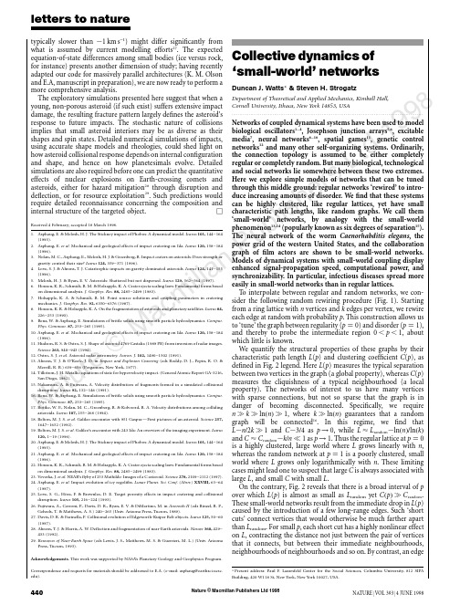
Nature © Macmillan Publishers Ltd 19988typically slower than ϳ1km s −1)might differ signiﬁcantly from what is assumed by current modelling efforts 27.The expected equation-of-state differences among small bodies (ice versus rock,for instance)presents another dimension of study;having recently adapted our code for massively parallel architectures (K.M.Olson and E.A,manuscript in preparation),we are now ready to perform a more comprehensive analysis.The exploratory simulations presented here suggest that when a young,non-porous asteroid (if such exist)suffers extensive impact damage,the resulting fracture pattern largely deﬁnes the asteroid’s response to future impacts.The stochastic nature of collisions implies that small asteroid interiors may be as diverse as their shapes and spin states.Detailed numerical simulations of impacts,using accurate shape models and rheologies,could shed light on how asteroid collisional response depends on internal conﬁguration and shape,and hence on how planetesimals evolve.Detailed simulations are also required before one can predict the quantitative effects of nuclear explosions on Earth-crossing comets and asteroids,either for hazard mitigation 28through disruption and deﬂection,or for resource exploitation 29.Such predictions would require detailed reconnaissance concerning the composition andinternal structure of the targeted object.ⅪReceived 4February;accepted 18March 1998.1.Asphaug,E.&Melosh,H.J.The Stickney impact of Phobos:A dynamical model.Icarus 101,144–164(1993).2.Asphaug,E.et al .Mechanical and geological effects of impact cratering on Ida.Icarus 120,158–184(1996).3.Nolan,M.C.,Asphaug,E.,Melosh,H.J.&Greenberg,R.Impact craters on asteroids:Does strength orgravity control their size?Icarus 124,359–371(1996).4.Love,S.J.&Ahrens,T.J.Catastrophic impacts on gravity dominated asteroids.Icarus 124,141–155(1996).5.Melosh,H.J.&Ryan,E.V.Asteroids:Shattered but not dispersed.Icarus 129,562–564(1997).6.Housen,K.R.,Schmidt,R.M.&Holsapple,K.A.Crater ejecta scaling laws:Fundamental forms basedon dimensional analysis.J.Geophys.Res.88,2485–2499(1983).7.Holsapple,K.A.&Schmidt,R.M.Point source solutions and coupling parameters in crateringmechanics.J.Geophys.Res.92,6350–6376(1987).8.Housen,K.R.&Holsapple,K.A.On the fragmentation of asteroids and planetary satellites.Icarus 84,226–253(1990).9.Benz,W.&Asphaug,E.Simulations of brittle solids using smooth particle put.mun.87,253–265(1995).10.Asphaug,E.et al .Mechanical and geological effects of impact cratering on Ida.Icarus 120,158–184(1996).11.Hudson,R.S.&Ostro,S.J.Shape of asteroid 4769Castalia (1989PB)from inversion of radar images.Science 263,940–943(1994).12.Ostro,S.J.et al .Asteroid radar astrometry.Astron.J.102,1490–1502(1991).13.Ahrens,T.J.&O’Keefe,J.D.in Impact and Explosion Cratering (eds Roddy,D.J.,Pepin,R.O.&Merrill,R.B.)639–656(Pergamon,New York,1977).14.Tillotson,J.H.Metallic equations of state for hypervelocity impact.(General Atomic Report GA-3216,San Diego,1962).15.Nakamura,A.&Fujiwara,A.Velocity distribution of fragments formed in a simulated collisionaldisruption.Icarus 92,132–146(1991).16.Benz,W.&Asphaug,E.Simulations of brittle solids using smooth particle put.mun.87,253–265(1995).17.Bottke,W.F.,Nolan,M.C.,Greenberg,R.&Kolvoord,R.A.Velocity distributions among collidingasteroids.Icarus 107,255–268(1994).18.Belton,M.J.S.et al .Galileo encounter with 951Gaspra—First pictures of an asteroid.Science 257,1647–1652(1992).19.Belton,M.J.S.et al .Galileo’s encounter with 243Ida:An overview of the imaging experiment.Icarus120,1–19(1996).20.Asphaug,E.&Melosh,H.J.The Stickney impact of Phobos:A dynamical model.Icarus 101,144–164(1993).21.Asphaug,E.et al .Mechanical and geological effects of impact cratering on Ida.Icarus 120,158–184(1996).22.Housen,K.R.,Schmidt,R.M.&Holsapple,K.A.Crater ejecta scaling laws:Fundamental forms basedon dimensional analysis.J.Geophys.Res.88,2485–2499(1983).23.Veverka,J.et al .NEAR’s ﬂyby of 253Mathilde:Images of a C asteroid.Science 278,2109–2112(1997).24.Asphaug,E.et al .Impact evolution of icy regoliths.Lunar Planet.Sci.Conf.(Abstr.)XXVIII,63–64(1997).25.Love,S.G.,Ho¨rz,F.&Brownlee,D.E.Target porosity effects in impact cratering and collisional disruption.Icarus 105,216–224(1993).26.Fujiwara,A.,Cerroni,P .,Davis,D.R.,Ryan,E.V.&DiMartino,M.in Asteroids II (eds Binzel,R.P .,Gehrels,T.&Matthews,A.S.)240–265(Univ.Arizona Press,Tucson,1989).27.Davis,D.R.&Farinella,P.Collisional evolution of Edgeworth-Kuiper Belt objects.Icarus 125,50–60(1997).28.Ahrens,T.J.&Harris,A.W.Deﬂection and fragmentation of near-Earth asteroids.Nature 360,429–433(1992).29.Resources of Near-Earth Space (eds Lewis,J.S.,Matthews,M.S.&Guerrieri,M.L.)(Univ.ArizonaPress,Tucson,1993).Acknowledgements.This work was supported by NASA’s Planetary Geology and Geophysics Program.Correspondence and requests for materials should be addressed to E.A.(e-mail:asphaug@).letters to nature440NATURE |VOL 393|4JUNE 1998Collective dynamics of ‘small-world’networksDuncan J.Watts *&Steven H.StrogatzDepartment of Theoretical and Applied Mechanics,Kimball Hall,Cornell University,Ithaca,New York 14853,USA.........................................................................................................................Networks of coupled dynamical systems have been used to model biological oscillators 1–4,Josephson junction arrays 5,6,excitable media 7,neural networks 8–10,spatial games 11,genetic control networks 12and many other self-organizing systems.Ordinarily,the connection topology is assumed to be either completely regular or completely random.But many biological,technological and social networks lie somewhere between these two extremes.Here we explore simple models of networks that can be tuned through this middle ground:regular networks ‘rewired’to intro-duce increasing amounts of disorder.We ﬁnd that these systems can be highly clustered,like regular lattices,yet have small characteristic path lengths,like random graphs.We call them ‘small-world’networks,by analogy with the small-world phenomenon 13,14(popularly known as six degrees of separation 15).The neural network of the worm Caenorhabditis elegans ,the power grid of the western United States,and the collaboration graph of ﬁlm actors are shown to be small-world networks.Models of dynamical systems with small-world coupling display enhanced signal-propagation speed,computational power,and synchronizability.In particular,infectious diseases spread more easily in small-world networks than in regular lattices.To interpolate between regular and random networks,we con-sider the following random rewiring procedure (Fig.1).Starting from a ring lattice with n vertices and k edges per vertex,we rewire each edge at random with probability p .This construction allows us to ‘tune’the graph between regularity (p ¼0)and disorder (p ¼1),and thereby to probe the intermediate region 0Ͻp Ͻ1,about which little is known.We quantify the structural properties of these graphs by their characteristic path length L (p )and clustering coefﬁcient C (p ),as deﬁned in Fig.2legend.Here L (p )measures the typical separation between two vertices in the graph (a global property),whereas C (p )measures the cliquishness of a typical neighbourhood (a local property).The networks of interest to us have many vertices with sparse connections,but not so sparse that the graph is in danger of becoming disconnected.Speciﬁcally,we require n q k q ln ðn Þq 1,where k q ln ðn Þguarantees that a random graph will be connected 16.In this regime,we ﬁnd that L ϳn =2k q 1and C ϳ3=4as p →0,while L ϷL random ϳln ðn Þ=ln ðk Þand C ϷC random ϳk =n p 1as p →1.Thus the regular lattice at p ¼0is a highly clustered,large world where L grows linearly with n ,whereas the random network at p ¼1is a poorly clustered,small world where L grows only logarithmically with n .These limiting cases might lead one to suspect that large C is always associated with large L ,and small C with small L .On the contrary,Fig.2reveals that there is a broad interval of p over which L (p )is almost as small as L random yet C ðp Þq C random .These small-world networks result from the immediate drop in L (p )caused by the introduction of a few long-range edges.Such ‘short cuts’connect vertices that would otherwise be much farther apart than L random .For small p ,each short cut has a highly nonlinear effect on L ,contracting the distance not just between the pair of vertices that it connects,but between their immediate neighbourhoods,neighbourhoods of neighbourhoods and so on.By contrast,an edge*Present address:Paul zarsfeld Center for the Social Sciences,Columbia University,812SIPA Building,420W118St,New York,New York 10027,USA.Nature © Macmillan Publishers Ltd 19988letters to natureNATURE |VOL 393|4JUNE 1998441removed from a clustered neighbourhood to make a short cut has,at most,a linear effect on C ;hence C (p )remains practically unchanged for small p even though L (p )drops rapidly.The important implica-tion here is that at the local level (as reﬂected by C (p )),the transition to a small world is almost undetectable.To check the robustness of these results,we have tested many different types of initial regular graphs,as well as different algorithms for random rewiring,and all give qualitatively similar results.The only requirement is that the rewired edges must typically connect vertices that would otherwise be much farther apart than L random .The idealized construction above reveals the key role of short cuts.It suggests that the small-world phenomenon might be common in sparse networks with many vertices,as even a tiny fraction of short cuts would sufﬁce.To test this idea,we have computed L and C for the collaboration graph of actors in feature ﬁlms (generated from data available at ),the electrical power grid of the western United States,and the neural network of the nematode worm C.elegans 17.All three graphs are of scientiﬁc interest.The graph of ﬁlm actors is a surrogate for a social network 18,with the advantage of being much more easily speciﬁed.It is also akin to the graph of mathematical collaborations centred,traditionally,on P.Erdo¨s (partial data available at /ϳgrossman/erdoshp.html).The graph of the power grid is relevant to the efﬁciency and robustness of power networks 19.And C.elegans is the sole example of a completely mapped neural network.Table 1shows that all three graphs are small-world networks.These examples were not hand-picked;they were chosen because of their inherent interest and because complete wiring diagrams were available.Thus the small-world phenomenon is not merely a curiosity of social networks 13,14nor an artefact of an idealizedmodel—it is probably generic for many large,sparse networks found in nature.We now investigate the functional signiﬁcance of small-world connectivity for dynamical systems.Our test case is a deliberately simpliﬁed model for the spread of an infectious disease.The population structure is modelled by the family of graphs described in Fig.1.At time t ¼0,a single infective individual is introduced into an otherwise healthy population.Infective individuals are removed permanently (by immunity or death)after a period of sickness that lasts one unit of dimensionless time.During this time,each infective individual can infect each of its healthy neighbours with probability r .On subsequent time steps,the disease spreads along the edges of the graph until it either infects the entire population,or it dies out,having infected some fraction of the population in theprocess.p = 0p = 1Regular Small-worldRandomFigure 1Random rewiring procedure for interpolating between a regular ring lattice and a random network,without altering the number of vertices or edges in the graph.We start with a ring of n vertices,each connected to its k nearest neighbours by undirected edges.(For clarity,n ¼20and k ¼4in the schematic examples shown here,but much larger n and k are used in the rest of this Letter.)We choose a vertex and the edge that connects it to its nearest neighbour in a clockwise sense.With probability p ,we reconnect this edge to a vertex chosen uniformly at random over the entire ring,with duplicate edges forbidden;other-wise we leave the edge in place.We repeat this process by moving clockwise around the ring,considering each vertex in turn until one lap is completed.Next,we consider the edges that connect vertices to their second-nearest neighbours clockwise.As before,we randomly rewire each of these edges with probability p ,and continue this process,circulating around the ring and proceeding outward to more distant neighbours after each lap,until each edge in the original lattice has been considered once.(As there are nk /2edges in the entire graph,the rewiring process stops after k /2laps.)Three realizations of this process are shown,for different values of p .For p ¼0,the original ring is unchanged;as p increases,the graph becomes increasingly disordered until for p ¼1,all edges are rewired randomly.One of our main results is that for intermediate values of p ,the graph is a small-world network:highly clustered like a regular graph,yet with small characteristic path length,like a random graph.(See Fig.2.)T able 1Empirical examples of small-world networksL actual L random C actual C random.............................................................................................................................................................................Film actors 3.65 2.990.790.00027Power grid 18.712.40.0800.005C.elegans 2.65 2.250.280.05.............................................................................................................................................................................Characteristic path length L and clustering coefﬁcient C for three real networks,compared to random graphs with the same number of vertices (n )and average number of edges per vertex (k ).(Actors:n ¼225;226,k ¼61.Power grid:n ¼4;941,k ¼2:67.C.elegans :n ¼282,k ¼14.)The graphs are deﬁned as follows.Two actors are joined by an edge if they have acted in a ﬁlm together.We restrict attention to the giant connected component 16of this graph,which includes ϳ90%of all actors listed in the Internet Movie Database (available at ),as of April 1997.For the power grid,vertices represent generators,transformers and substations,and edges represent high-voltage transmission lines between them.For C.elegans ,an edge joins two neurons if they are connected by either a synapse or a gap junction.We treat all edges as undirected and unweighted,and all vertices as identical,recognizing that these are crude approximations.All three networks show the small-world phenomenon:L ՌL random but C q C random.00.20.40.60.810.00010.0010.010.11pFigure 2Characteristic path length L (p )and clustering coefﬁcient C (p )for the family of randomly rewired graphs described in Fig.1.Here L is deﬁned as the number of edges in the shortest path between two vertices,averaged over all pairs of vertices.The clustering coefﬁcient C (p )is deﬁned as follows.Suppose that a vertex v has k v neighbours;then at most k v ðk v Ϫ1Þ=2edges can exist between them (this occurs when every neighbour of v is connected to every other neighbour of v ).Let C v denote the fraction of these allowable edges that actually exist.Deﬁne C as the average of C v over all v .For friendship networks,these statistics have intuitive meanings:L is the average number of friendships in the shortest chain connecting two people;C v reﬂects the extent to which friends of v are also friends of each other;and thus C measures the cliquishness of a typical friendship circle.The data shown in the ﬁgure are averages over 20random realizations of the rewiring process described in Fig.1,and have been normalized by the values L (0),C (0)for a regular lattice.All the graphs have n ¼1;000vertices and an average degree of k ¼10edges per vertex.We note that a logarithmic horizontal scale has been used to resolve the rapid drop in L (p ),corresponding to the onset of the small-world phenomenon.During this drop,C (p )remains almost constant at its value for the regular lattice,indicating that the transition to a small world is almost undetectable at the local level.Nature © Macmillan Publishers Ltd 19988letters to nature442NATURE |VOL 393|4JUNE 1998Two results emerge.First,the critical infectiousness r half ,at which the disease infects half the population,decreases rapidly for small p (Fig.3a).Second,for a disease that is sufﬁciently infectious to infect the entire population regardless of its structure,the time T (p )required for global infection resembles the L (p )curve (Fig.3b).Thus,infectious diseases are predicted to spread much more easily and quickly in a small world;the alarming and less obvious point is how few short cuts are needed to make the world small.Our model differs in some signiﬁcant ways from other network models of disease spreading 20–24.All the models indicate that net-work structure inﬂuences the speed and extent of disease transmis-sion,but our model illuminates the dynamics as an explicit function of structure (Fig.3),rather than for a few particular topologies,such as random graphs,stars and chains 20–23.In the work closest to ours,Kretschmar and Morris 24have shown that increases in the number of concurrent partnerships can signiﬁcantly accelerate the propaga-tion of a sexually-transmitted disease that spreads along the edges of a graph.All their graphs are disconnected because they ﬁx the average number of partners per person at k ¼1.An increase in the number of concurrent partnerships causes faster spreading by increasing the number of vertices in the graph’s largest connected component.In contrast,all our graphs are connected;hence the predicted changes in the spreading dynamics are due to more subtle structural features than changes in connectedness.Moreover,changes in the number of concurrent partners are obvious to an individual,whereas transitions leading to a smaller world are not.We have also examined the effect of small-world connectivity on three other dynamical systems.In each case,the elements were coupled according to the family of graphs described in Fig.1.(1)For cellular automata charged with the computational task of density classiﬁcation 25,we ﬁnd that a simple ‘majority-rule’running on a small-world graph can outperform all known human and genetic algorithm-generated rules running on a ring lattice.(2)For the iterated,multi-player ‘Prisoner’s dilemma’11played on a graph,we ﬁnd that as the fraction of short cuts increases,cooperation is less likely to emerge in a population of players using a generalized ‘tit-for-tat’26strategy.The likelihood of cooperative strategies evolving out of an initial cooperative/non-cooperative mix also decreases with increasing p .(3)Small-world networks of coupled phase oscillators synchronize almost as readily as in the mean-ﬁeld model 2,despite having orders of magnitude fewer edges.This result may be relevant to the observed synchronization of widely separated neurons in the visual cortex 27if,as seems plausible,the brain has a small-world architecture.We hope that our work will stimulate further studies of small-world networks.Their distinctive combination of high clustering with short characteristic path length cannot be captured by traditional approximations such as those based on regular lattices or random graphs.Although small-world architecture has not received much attention,we suggest that it will probably turn out to be widespread in biological,social and man-made systems,oftenwith important dynamical consequences.ⅪReceived 27November 1997;accepted 6April 1998.1.Winfree,A.T.The Geometry of Biological Time (Springer,New Y ork,1980).2.Kuramoto,Y.Chemical Oscillations,Waves,and Turbulence (Springer,Berlin,1984).3.Strogatz,S.H.&Stewart,I.Coupled oscillators and biological synchronization.Sci.Am.269(6),102–109(1993).4.Bressloff,P .C.,Coombes,S.&De Souza,B.Dynamics of a ring of pulse-coupled oscillators:a group theoretic approach.Phys.Rev.Lett.79,2791–2794(1997).5.Braiman,Y.,Lindner,J.F.&Ditto,W.L.Taming spatiotemporal chaos with disorder.Nature 378,465–467(1995).6.Wiesenfeld,K.New results on frequency-locking dynamics of disordered Josephson arrays.Physica B 222,315–319(1996).7.Gerhardt,M.,Schuster,H.&Tyson,J.J.A cellular automaton model of excitable media including curvature and dispersion.Science 247,1563–1566(1990).8.Collins,J.J.,Chow,C.C.&Imhoff,T.T.Stochastic resonance without tuning.Nature 376,236–238(1995).9.Hopﬁeld,J.J.&Herz,A.V.M.Rapid local synchronization of action potentials:Toward computation with coupled integrate-and-ﬁre neurons.Proc.Natl A 92,6655–6662(1995).10.Abbott,L.F.&van Vreeswijk,C.Asynchronous states in neural networks of pulse-coupled oscillators.Phys.Rev.E 48(2),1483–1490(1993).11.Nowak,M.A.&May,R.M.Evolutionary games and spatial chaos.Nature 359,826–829(1992).12.Kauffman,S.A.Metabolic stability and epigenesis in randomly constructed genetic nets.J.Theor.Biol.22,437–467(1969).gram,S.The small world problem.Psychol.Today 2,60–67(1967).14.Kochen,M.(ed.)The Small World (Ablex,Norwood,NJ,1989).15.Guare,J.Six Degrees of Separation:A Play (Vintage Books,New Y ork,1990).16.Bollaba´s,B.Random Graphs (Academic,London,1985).17.Achacoso,T.B.&Yamamoto,W.S.AY’s Neuroanatomy of C.elegans for Computation (CRC Press,BocaRaton,FL,1992).18.Wasserman,S.&Faust,K.Social Network Analysis:Methods and Applications (Cambridge Univ.Press,1994).19.Phadke,A.G.&Thorp,puter Relaying for Power Systems (Wiley,New Y ork,1988).20.Sattenspiel,L.&Simon,C.P .The spread and persistence of infectious diseases in structured populations.Math.Biosci.90,341–366(1988).21.Longini,I.M.Jr A mathematical model for predicting the geographic spread of new infectious agents.Math.Biosci.90,367–383(1988).22.Hess,G.Disease in metapopulation models:implications for conservation.Ecology 77,1617–1632(1996).23.Blythe,S.P .,Castillo-Chavez,C.&Palmer,J.S.T oward a uniﬁed theory of sexual mixing and pair formation.Math.Biosci.107,379–405(1991).24.Kretschmar,M.&Morris,M.Measures of concurrency in networks and the spread of infectious disease.Math.Biosci.133,165–195(1996).25.Das,R.,Mitchell,M.&Crutchﬁeld,J.P .in Parallel Problem Solving from Nature (eds Davido,Y.,Schwefel,H.-P.&Ma¨nner,R.)344–353(Lecture Notes in Computer Science 866,Springer,Berlin,1994).26.Axelrod,R.The Evolution of Cooperation (Basic Books,New Y ork,1984).27.Gray,C.M.,Ko¨nig,P .,Engel,A.K.&Singer,W.Oscillatory responses in cat visual cortex exhibit inter-columnar synchronization which reﬂects global stimulus properties.Nature 338,334–337(1989).Acknowledgements.We thank B.Tjaden for providing the ﬁlm actor data,and J.Thorp and K.Bae for the Western States Power Grid data.This work was supported by the US National Science Foundation (Division of Mathematical Sciences).Correspondence and requests for materials should be addressed to D.J.W.(e-mail:djw24@).0.150.20.250.30.350.00010.0010.010.11rhalfpaFigure 3Simulation results for a simple model of disease spreading.The community structure is given by one realization of the family of randomly rewired graphs used in Fig.1.a ,Critical infectiousness r half ,at which the disease infects half the population,decreases with p .b ,The time T (p )required for a maximally infectious disease (r ¼1)to spread throughout the entire population has essen-tially the same functional form as the characteristic path length L (p ).Even if only a few per cent of the edges in the original lattice are randomly rewired,the time to global infection is nearly as short as for a random graph.0.20.40.60.810.00010.0010.010.11pb。

抽样方案的种类包括什么

抽样方案的种类包括什么抽样方案的种类包括什么摘要：抽样是统计学中的一项重要方法，用于从总体中选择一部分样本进行研究和分析。

抽样方案的选择和设计对于研究结果的准确性和可靠性具有决定性的影响。

本文将介绍抽样方案的种类，包括简单随机抽样、系统抽样、整群抽样、分层抽样、多阶段抽样和方便抽样，并对其特点和应用进行详细阐述。

一、简单随机抽样简单随机抽样是最基本的抽样方法，是通过随机抽取每个样本的概率相等，且相互独立的方法。

该方法的优点是样本选择的公平性和随机性，能够较好地代表总体的特征。

然而，由于随机性的特点，样本容易出现偏差，因此需要在实际应用中进行适当的校正和控制。

二、系统抽样系统抽样是按照一定的规则和顺序从总体中抽取样本的方法。

该方法的优点是简单、快捷，能够保持总体的一定特征，并且可以避免简单随机抽样中可能出现的偏差。

然而，如果总体中存在周期性或规律性的特征，系统抽样可能导致样本偏差。

三、整群抽样整群抽样是将总体划分为若干个互不重叠的群体，然后从每个群体中选择部分群体进行抽样的方法。

该方法的优点是能够更好地反映总体的特征，并且减少样本选择的复杂性。

然而，由于群体内的个体可能存在差异，整群抽样可能导致样本的偏差。

四、分层抽样分层抽样是将总体划分为若干个相互独立的层次，然后从每个层次中选择部分样本进行抽样的方法。

该方法的优点是能够在样本选择中考虑到不同层次的差异，增加样本的多样性，并且可以更好地反映总体的特征。

然而，分层抽样需要事先知道总体的分层特征，否则可能导致样本的偏差。

五、多阶段抽样多阶段抽样是将总体分为多个阶段，然后在每个阶段中选择部分样本进行抽样的方法。

该方法的优点是能够逐步缩小样本范围，减少样本选择的复杂性，并且节约时间和成本。

然而，多阶段抽样可能导致样本的聚集性和偏差，需要在设计中合理考虑和控制。

六、方便抽样方便抽样是基于研究者的便利性和容易获得的样本进行抽样的方法。

该方法的优点是简单、快捷，适用于一些初步研究或实践中的问题。

市场调查方法(英文版)第十五章

15–14
EXHIBIT 15.2 Independent Samples t-Test Results
© 2007 Thomson/South-Western. All rights reserved.
15–15
What Is ANOVA?
• Analysis of Variance (ANOVA)
➢ An analysis involving the investigation of the effects of one treatment variable on an interval-scaled dependent variable
➢ A hypothesis-testing technique to determine whether statistically significant differences in means occur between two or more groups.
❖ Behavior, characteristics, beliefs, opinions, emotions, or attitudes
• Bivariate Tests of Differences
➢ Involve only two variables: a variable that acts like a dependent variable and a variable that acts as a classification variable.
❖ Differences in mean scores between groups or in comparing how two groups’ scores are distributed across possible response categories.

计量经济学导论CH13习题答案

CHAPTER 13TEACHING NOTESWhile this chapter falls under “Advanced Topics,” most of this chapter requires no more sophistication than the previous chapters. (In fact, I would argue that, with the possible exception of Section 13.5, this material is easier than some of the time series chapters.)Pooling two or more independent cross sections is a straightforward extension of cross-sectional methods. Nothing new needs to be done in stating assumptions, except possibly mentioning that random sampling in each time period is sufficient. The practically important issue is allowing for different intercepts, and possibly different slopes, across time.The natural experiment material and extensions of the difference-in-differences estimator is widely applicable and, with the aid of the examples, easy to understand.Two years of panel data are often available, in which case differencing across time is a simple way of removing g unobserved heterogeneity. If you have covered Chapter 9, you might compare this with a regression in levels using the second year of data, but where a lagged dependent variable is included. (The second approach only requires collecting information on the dependent variable in a previous year.) These often give similar answers. Two years of panel data, collected before and after a policy change, can be very powerful for policy analysis. Having more than two periods of panel data causes slight complications in that the errors in the differenced equation may be serially correlated. (However, the traditional assumption that the errors in the original equation are serially uncorrelated is not always a good one. In other words, it is not always more appropriate to used fixed effects, as in Chapter 14, than first differencing.) With large N and relatively small T, a simple way to account for possible serial correlation after differencing is to compute standard errors that are robust to arbitrary serial correlation and heteroskedasticity. Econometrics packages that do cluster analysis (such as Stata) often allow this by specifying each cross-sectional unit as its own cluster.108SOLUTIONS TO PROBLEMS13.1 Without changes in the averages of any explanatory variables, the average fertility rate fellby .545 between 1972 and 1984; this is simply the coefficient on y84. To account for theincrease in average education levels, we obtain an additional effect: –.128(13.3 – 12.2) ≈–.141. So the drop in average fertility if the average education level increased by 1.1 is .545+ .141 = .686, or roughly two-thirds of a child per woman.13.2 The first equation omits the 1981 year dummy variable, y81, and so does not allow anyappreciation in nominal housing prices over the three year period in the absence of an incinerator. The interaction term in this case is simply picking up the fact that even homes that are near the incinerator site have appreciated in value over the three years. This equation suffers from omitted variable bias.The second equation omits the dummy variable for being near the incinerator site, nearinc,which means it does not allow for systematic differences in homes near and far from the sitebefore the site was built. If, as seems to be the case, the incinerator was located closer to lessvaluable homes, then omitting nearinc attributes lower housing prices too much to theincinerator effect. Again, we have an omitted variable problem. This is why equation (13.9) (or,even better, the equation that adds a full set of controls), is preferred.13.3 We do not have repeated observations on the same cross-sectional units in each time period,and so it makes no sense to look for pairs to difference. For example, in Example 13.1, it is veryunlikely that the same woman appears in more than one year, as new random samples areobtained in each year. In Example 13.3, some houses may appear in the sample for both 1978and 1981, but the overlap is usually too small to do a true panel data analysis.β, but only13.4 The sign of β1 does not affect the direction of bias in the OLS estimator of1whether we underestimate or overestimate the effect of interest. If we write ∆crmrte i = δ0 +β1∆unem i + ∆u i, where ∆u i and ∆unem i are negatively correlated, then there is a downward biasin the OLS estimator of β1. Because β1 > 0, we will tend to underestimate the effect of unemployment on crime.13.5 No, we cannot include age as an explanatory variable in the original model. Each person inthe panel data set is exactly two years older on January 31, 1992 than on January 31, 1990. This means that ∆age i = 2 for all i. But the equation we would estimate is of the form∆saving i = δ0 + β1∆age i +…,where δ0 is the coefficient the year dummy for 1992 in the original model. As we know, whenwe have an intercept in the model we cannot include an explanatory variable that is constant across i; this violates Assumption MLR.3. Intuitively, since age changes by the same amount for everyone, we cannot distinguish the effect of age from the aggregate time effect.10913.6 (i) Let FL be a binary variable equal to one if a person lives in Florida, and zero otherwise. Let y90 be a year dummy variable for 1990. Then, from equation (13.10), we have the linear probability modelarrest = β0 + δ0y90 + β1FL + δ1y90⋅FL + u.The effect of the law is measured by δ1, which is the change in the probability of drunk driving arrest due to the new law in Florida. Including y90 allows for aggregate trends in drunk driving arrests that would affect both states; including FL allows for systematic differences between Florida and Georgia in either drunk driving behavior or law enforcement.(ii) It could be that the populations of drivers in the two states change in different ways over time. For example, age, race, or gender distributions may have changed. The levels of education across the two states may have changed. As these factors might affect whether someone is arrested for drunk driving, it could be important to control for them. At a minimum, there is the possibility of obtaining a more precise estimator of δ1 by reducing the error variance. Essentially, any explanatory variable that affects arrest can be used for this purpose. (See Section 6.3 for discussion.)SOLUTIONS TO COMPUTER EXERCISES13.7 (i) The F statistic (with 4 and 1,111 df) is about 1.16 and p-value ≈ .328, which shows that the living environment variables are jointly insignificant.(ii) The F statistic (with 3 and 1,111 df) is about 3.01 and p-value ≈ .029, and so the region dummy variables are jointly significant at the 5% level.(iii) After obtaining the OLS residuals, ˆu, from estimating the model in Table 13.1, we run the regression 2ˆu on y74, y76, …, y84 using all 1,129 observations. The null hypothesis of homoskedasticity is H0: γ1 = 0, γ2= 0, … , γ6 = 0. So we just use the usual F statistic for joint significance of the year dummies. The R-squared is about .0153 and F ≈ 2.90; with 6 and 1,122 df, the p-value is about .0082. So there is evidence of heteroskedasticity that is a function of time at the 1% significance level. This suggests that, at a minimum, we should compute heteroskedasticity-robust standard errors, t statistics, and F statistics. We could also use weighted least squares (although the form of heteroskedasticity used here may not be sufficient; it does not depend on educ, age, and so on).(iv) Adding y74⋅educ, , y84⋅educ allows the relationship between fertility and education to be different in each year; remember, the coefficient on the interaction gets added to the coefficient on educ to get the slope for the appropriate year. When these interaction terms are added to the equation, R2≈ .137. The F statistic for joint significance (with 6 and 1,105 df) is about 1.48 with p-value ≈ .18. Thus, the interactions are not jointly significant at even the 10% level. This is a bit misleading, however. An abbreviated equation (which just shows the coefficients on the terms involving educ) is110111kids= -8.48 - .023 educ + - .056 y74⋅educ - .092 y76⋅educ(3.13) (.054) (.073) (.071) - .152 y78⋅educ - .098 y80⋅educ - .139 y82⋅educ - .176 y84⋅educ .(.075) (.070) (.068) (.070)Three of the interaction terms, y78⋅educ , y82⋅educ , and y84⋅educ are statistically significant at the 5% level against a two-sided alternative, with the p -value on the latter being about .012. The coefficients are large in magnitude as well. The coefficient on educ – which is for the base year, 1972 – is small and insignificant, suggesting little if any relationship between fertility andeducation in the early seventies. The estimates above are consistent with fertility becoming more linked to education as the years pass. The F statistic is insignificant because we are testing some insignificant coefficients along with some significant ones.13.8 (i) The coefficient on y85 is roughly the proportionate change in wage for a male (female = 0) with zero years of education (educ = 0). This is not especially useful since we are not interested in people with no education.(ii) What we want to estimate is θ0 = δ0 + 12δ1; this is the change in the intercept for a male with 12 years of education, where we also hold other factors fixed. If we write δ0 = θ0 - 12δ1, plug this into (13.1), and rearrange, we getlog(wage ) = β0 + θ0y85 + β1educ + δ1y85⋅(educ – 12) + β2exper + β3exper 2 + β4union + β5female + δ5y85⋅female + u .Therefore, we simply replace y85⋅educ with y85⋅(educ – 12), and then the coefficient andstandard error we want is on y85. These turn out to be 0ˆθ = .339 and se(0ˆθ) = .034. Roughly, the nominal increase in wage is 33.9%, and the 95% confidence interval is 33.9 ± 1.96(3.4), or about 27.2% to 40.6%. (Because the proportionate change is large, we could use equation (7.10), which implies the point estimate 40.4%; but obtaining the standard error of this estimate is harder.)(iii) Only the coefficient on y85 differs from equation (13.2). The new coefficient is about –.383 (se ≈ .124). This shows that real wages have fallen over the seven year period, although less so for the more educated. For example, the proportionate change for a male with 12 years of education is –.383 + .0185(12) = -.161, or a fall of about 16.1%. For a male with 20 years of education there has been almost no change [–.383 + .0185(20) = –.013].(iv) The R -squared when log(rwage ) is the dependent variable is .356, as compared with .426 when log(wage ) is the dependent variable. If the SSRs from the regressions are the same, but the R -squareds are not, then the total sum of squares must be different. This is the case, as the dependent variables in the two equations are different.(v) In 1978, about 30.6% of workers in the sample belonged to a union. In 1985, only about 18% belonged to a union. Therefore, over the seven-year period, there was a notable fall in union membership.(vi) When y85⋅union is added to the equation, its coefficient and standard error are about -.00040 (se ≈ .06104). This is practically very small and the t statistic is almost zero. There has been no change in the union wage premium over time.(vii) Parts (v) and (vi) are not at odds. They imply that while the economic return to union membership has not changed (assuming we think we have estimated a causal effect), the fraction of people reaping those benefits has fallen.13.9 (i) Other things equal, homes farther from the incinerator should be worth more, so δ1 > 0. If β1 > 0, then the incinerator was located farther away from more expensive homes.(ii) The estimated equation islog()price= 8.06 -.011 y81+ .317 log(dist) + .048 y81⋅log(dist)(0.51) (.805) (.052) (.082)n = 321, R2 = .396, 2R = .390.ˆδ = .048 is the expected sign, it is not statistically significant (t statistic ≈ .59).While1(iii) When we add the list of housing characteristics to the regression, the coefficient ony81⋅log(dist) becomes .062 (se = .050). So the estimated effect is larger – the elasticity of price with respect to dist is .062 after the incinerator site was chosen – but its t statistic is only 1.24. The p-value for the one-sided alternative H1: δ1 > 0 is about .108, which is close to being significant at the 10% level.13.10 (i) In addition to male and married, we add the variables head, neck, upextr, trunk, lowback, lowextr, and occdis for injury type, and manuf and construc for industry. The coefficient on afchnge⋅highearn becomes .231 (se ≈ .070), and so the estimated effect and t statistic are now larger than when we omitted the control variables. The estimate .231 implies a substantial response of durat to the change in the cap for high-earnings workers.(ii) The R-squared is about .041, which means we are explaining only a 4.1% of the variation in log(durat). This means that there are some very important factors that affect log(durat) that we are not controlling for. While this means that predicting log(durat) would be very difficultˆδ: it could still for a particular individual, it does not mean that there is anything biased about1be an unbiased estimator of the causal effect of changing the earnings cap for workers’ compensation.(iii) The estimated equation using the Michigan data is112durat= 1.413 + .097 afchnge+ .169 highearn+ .192 afchnge⋅highearn log()(0.057) (.085) (.106) (.154)n = 1,524, R2 = .012.The estimate of δ1, .192, is remarkably close to the estimate obtained for Kentucky (.191). However, the standard error for the Michigan estimate is much higher (.154 compared with .069). The estimate for Michigan is not statistically significant at even the 10% level against δ1 > 0. Even though we have over 1,500 observations, we cannot get a very precise estimate. (For Kentucky, we have over 5,600 observations.)13.11 (i) Using pooled OLS we obtainrent= -.569 + .262 d90+ .041 log(pop) + .571 log(avginc) + .0050 pctstu log()(.535) (.035) (.023) (.053) (.0010) n = 128, R2 = .861.The positive and very significant coefficient on d90 simply means that, other things in the equation fixed, nominal rents grew by over 26% over the 10 year period. The coefficient on pctstu means that a one percentage point increase in pctstu increases rent by half a percent (.5%). The t statistic of five shows that, at least based on the usual analysis, pctstu is very statistically significant.(ii) The standard errors from part (i) are not valid, unless we thing a i does not really appear in the equation. If a i is in the error term, the errors across the two time periods for each city are positively correlated, and this invalidates the usual OLS standard errors and t statistics.(iii) The equation estimated in differences islog()∆= .386 + .072 ∆log(pop) + .310 log(avginc) + .0112 ∆pctsturent(.037) (.088) (.066) (.0041)n = 64, R2 = .322.Interestingly, the effect of pctstu is over twice as large as we estimated in the pooled OLS equation. Now, a one percentage point increase in pctstu is estimated to increase rental rates by about 1.1%. Not surprisingly, we obtain a much less precise estimate when we difference (although the OLS standard errors from part (i) are likely to be much too small because of the positive serial correlation in the errors within each city). While we have differenced away a i, there may be other unobservables that change over time and are correlated with ∆pctstu.(iv) The heteroskedasticity-robust standard error on ∆pctstu is about .0028, which is actually much smaller than the usual OLS standard error. This only makes pctstu even more significant (robust t statistic ≈ 4). Note that serial correlation is no longer an issue because we have no time component in the first-differenced equation.11311413.12 (i) You may use an econometrics software package that directly tests restrictions such as H 0: β1 = β2 after estimating the unrestricted model in (13.22). But, as we have seen many times, we can simply rewrite the equation to test this using any regression software. Write the differenced equation as∆log(crime ) = δ0 + β1∆clrprc -1 + β2∆clrprc -2 + ∆u .Following the hint, we define θ1 = β1 - β2, and then write β1 = θ1 + β2. Plugging this into the differenced equation and rearranging gives∆log(crime ) = δ0 + θ1∆clrprc -1 + β2(∆clrprc -1 + ∆clrprc -2) + ∆u .Estimating this equation by OLS gives 1ˆθ= .0091, se(1ˆθ) = .0085. The t statistic for H 0: β1 = β2 is .0091/.0085 ≈ 1.07, which is not statistically significant.(ii) With β1 = β2 the equation becomes (without the i subscript)∆log(crime ) = δ0 + β1(∆clrprc -1 + ∆clrprc -2) + ∆u= δ0 + δ1[(∆clrprc -1 + ∆clrprc -2)/2] + ∆u ,where δ1 = 2β1. But (∆clrprc -1 + ∆clrprc -2)/2 = ∆avgclr .(iii) The estimated equation islog()crime ∆ = .099 - .0167 ∆avgclr(.063) (.0051)n = 53, R 2 = .175, 2R = .159.Since we did not reject the hypothesis in part (i), we would be justified in using the simplermodel with avgclr . Based on adjusted R -squared, we have a slightly worse fit with the restriction imposed. But this is a minor consideration. Ideally, we could get more data to determine whether the fairly different unconstrained estimates of β1 and β2 in equation (13.22) reveal true differences in β1 and β2.13.13 (i) Pooling across semesters and using OLS givestrmgpa = -1.75 -.058 spring+ .00170 sat- .0087 hsperc(0.35) (.048) (.00015) (.0010)+ .350 female- .254 black- .023 white- .035 frstsem(.052) (.123) (.117) (.076)- .00034 tothrs + 1.048 crsgpa- .027 season(.00073) (0.104) (.049)n = 732, R2 = .478, 2R = .470.The coefficient on season implies that, other things fixed, an athlete’s term GPA is about .027 points lower when his/her sport is in season. On a four point scale, this a modest effect (although it accumulates over four years of athletic eligibility). However, the estimate is not statistically significant (t statistic ≈-.55).(ii) The quick answer is that if omitted ability is correlated with season then, as we know form Chapters 3 and 5, OLS is biased and inconsistent. The fact that we are pooling across two semesters does not change that basic point.If we think harder, the direction of the bias is not clear, and this is where pooling across semesters plays a role. First, suppose we used only the fall term, when football is in season. Then the error term and season would be negatively correlated, which produces a downward bias in the OLS estimator of βseason. Because βseason is hypothesized to be negative, an OLS regression using only the fall data produces a downward biased estimator. [When just the fall data are used, ˆβ = -.116 (se = .084), which is in the direction of more bias.] However, if we use just the seasonspring semester, the bias is in the opposite direction because ability and season would be positive correlated (more academically able athletes are in season in the spring). In fact, using just theβ = .00089 (se = .06480), which is practically and statistically equal spring semester gives ˆseasonto zero. When we pool the two semesters we cannot, with a much more detailed analysis, determine which bias will dominate.(iii) The variables sat, hsperc, female, black, and white all drop out because they do not vary by semester. The intercept in the first-differenced equation is the intercept for the spring. We have∆= -.237 + .019 ∆frstsem+ .012 ∆tothrs+ 1.136 ∆crsgpa- .065 seasontrmgpa(.206) (.069) (.014) (0.119) (.043) n = 366, R2 = .208, 2R = .199.Interestingly, the in-season effect is larger now: term GPA is estimated to be about .065 points lower in a semester that the sport is in-season. The t statistic is about –1.51, which gives a one-sided p-value of about .065.115(iv) One possibility is a measure of course load. If some fraction of student-athletes take a lighter load during the season (for those sports that have a true season), then term GPAs may tend to be higher, other things equal. This would bias the results away from finding an effect of season on term GPA.13.14 (i) The estimated equation using differences is∆= -2.56 - 1.29 ∆log(inexp) - .599 ∆log(chexp) + .156 ∆incshrvote(0.63) (1.38) (.711) (.064)n = 157, R2 = .244, 2R = .229.Only ∆incshr is statistically significant at the 5% level (t statistic ≈ 2.44, p-value ≈ .016). The other two independent variables have t statistics less than one in absolute value.(ii) The F statistic (with 2 and 153 df) is about 1.51 with p-value ≈ .224. Therefore,∆log(inexp) and ∆log(chexp) are jointly insignificant at even the 20% level.(iii) The simple regression equation is∆= -2.68 + .218 ∆incshrvote(0.63) (.032)n = 157, R2 = .229, 2R = .224.This equation implies t hat a 10 percentage point increase in the incumbent’s share of total spending increases the percent of the incumbent’s vote by about 2.2 percentage points.(iv) Using the 33 elections with repeat challengers we obtain∆= -2.25 + .092 ∆incshrvote(1.00) (.085)n = 33, R2 = .037, 2R = .006.The estimated effect is notably smaller and, not surprisingly, the standard error is much larger than in part (iii). While the direction of the effect is the same, it is not statistically significant (p-value ≈ .14 against a one-sided alternative).13.15 (i) When we add the changes of the nine log wage variables to equation (13.33) we obtain116117 log()crmrte ∆ = .020 - .111 d83 - .037 d84 - .0006 d85 + .031 d86 + .039 d87(.021) (.027) (.025) (.0241) (.025) (.025)- .323 ∆log(prbarr ) - .240 ∆log(prbconv ) - .169 ∆log(prbpris )(.030) (.018) (.026)- .016 ∆log(avgsen ) + .398 ∆log(polpc ) - .044 ∆log(wcon )(.022) (.027) (.030)+ .025 ∆log(wtuc ) - .029 ∆log(wtrd ) + .0091 ∆log(wfir )(0.14) (.031) (.0212)+ .022 ∆log(wser ) - .140 ∆log(wmfg ) - .017 ∆log(wfed )(.014) (.102) (.172)- .052 ∆log(wsta ) - .031 ∆log(wloc ) (.096) (.102) n = 540, R 2 = .445, 2R = .424.The coefficients on the criminal justice variables change very modestly, and the statistical significance of each variable is also essentially unaffected.(ii) Since some signs are positive and others are negative, they cannot all really have the expected sign. For example, why is the coefficient on the wage for transportation, utilities, and communications (wtuc ) positive and marginally significant (t statistic ≈ 1.79)? Higher manufacturing wages lead to lower crime, as we might expect, but, while the estimated coefficient is by far the largest in magnitude, it is not statistically different from zero (tstatistic ≈ –1.37). The F test for joint significance of the wage variables, with 9 and 529 df , yields F ≈ 1.25 and p -value ≈ .26.13.16 (i) The estimated equation using the 1987 to 1988 and 1988 to 1989 changes, where we include a year dummy for 1989 in addition to an overall intercept, isˆhrsemp ∆ = –.740 + 5.42 d89 + 32.60 ∆grant + 2.00 ∆grant -1 + .744 ∆log(employ ) (1.942) (2.65) (2.97) (5.55) (4.868)n = 251, R 2 = .476, 2R = .467.There are 124 firms with both years of data and three firms with only one year of data used, for a total of 127 firms; 30 firms in the sample have missing information in both years and are not used at all. If we had information for all 157 firms, we would have 314 total observations in estimating the equation.(ii) The coefficient on grant – more precisely, on ∆grant in the differenced equation – means that if a firm received a grant for the current year, it trained each worker an average of 32.6 hoursmore than it would have otherwise. This is a practically large effect, and the t statistic is very large.(iii) Since a grant last year was used to pay for training last year, it is perhaps not surprising that the grant does not carry over into more training this year. It would if inertia played a role in training workers.(iv) The coefficient on the employees variable is very small: a 10% increase in employ increases hours per employee by only .074. [Recall:∆≈ (.744/100)(%∆employ).] Thishrsempis very small, and the t statistic is also rather small.13.17. (i) Take changes as usual, holding the other variables fixed: ∆math4it = β1∆log(rexpp it) = (β1/100)⋅[ 100⋅∆log(rexpp it)] ≈ (β1/100)⋅( %∆rexpp it). So, if %∆rexpp it = 10, then ∆math4it= (β1/100)⋅(10) = β1/10.(ii) The equation, estimated by pooled OLS in first differences (except for the year dummies), is4∆ = 5.95 + .52 y94 + 6.81 y95- 5.23 y96- 8.49 y97 + 8.97 y98math(.52) (.73) (.78) (.73) (.72) (.72)- 3.45 ∆log(rexpp) + .635 ∆log(enroll) + .025 ∆lunch(2.76) (1.029) (.055)n = 3,300, R2 = .208.Taken literally, the spending coefficient implies that a 10% increase in real spending per pupil decreases the math4 pass rate by about 3.45/10 ≈ .35 percentage points.(iii) When we add the lagged spending change, and drop another year, we get4∆ = 6.16 + 5.70 y95- 6.80 y96- 8.99 y97 +8.45 y98math(.55) (.77) (.79) (.74) (.74)- 1.41 ∆log(rexpp) + 11.04 ∆log(rexpp-1) + 2.14 ∆log(enroll)(3.04) (2.79) (1.18)+ .073 ∆lunch(.061)n = 2,750, R2 = .238.The contemporaneous spending variable, while still having a negative coefficient, is not at all statistically significant. The coefficient on the lagged spending variable is very statistically significant, and implies that a 10% increase in spending last year increases the math4 pass rate118119 by about 1.1 percentage points. Given the timing of the tests, a lagged effect is not surprising. In Michigan, the fourth grade math test is given in January, and so if preparation for the test begins a full year in advance, spending when the students are in third grade would at least partly matter.(iv) The heteroskedasticity-robust standard error for log() ˆrexpp β∆is about 4.28, which reducesthe significance of ∆log(rexpp ) even further. The heteroskedasticity-robust standard error of 1log() ˆrexpp β-∆is about 4.38, which substantially lowers the t statistic. Still, ∆log(rexpp -1) is statistically significant at just over the 1% significance level against a two-sided alternative.(v) The fully robust standard error for log() ˆrexpp β∆is about 4.94, which even further reducesthe t statistic for ∆log(rexpp ). The fully robust standard error for 1log() ˆrexpp β-∆is about 5.13,which gives ∆log(rexpp -1) a t statistic of about 2.15. The two-sided p -value is about .032.(vi) We can use four years of data for this test. Doing a pooled OLS regression of ,1垐 on it i t r r -,using years 1995, 1996, 1997, and 1998 gives ˆρ= -.423 (se = .019), which is strong negative serial correlation.(vii) Th e fully robust “F ” test for ∆log(enroll ) and ∆lunch , reported by Stata 7.0, is .93. With 2 and 549 df , this translates into p -value = .40. So we would be justified in dropping these variables, but they are not doing any harm.。

雅思阅读机经真题解析-Novice and Expert

雅思阅读机经真题解析-Novice and Expert小站独家，雅思阅读机经真题解析。

一切患有雅思阅读刷题强迫症的烤鸭，请看这里。

小站精心整理了一批雅思阅读机经真题。

如果你的剑桥雅思阅读已是烂熟于心，那么这一系列的雅思阅读机经真题真的很适合你，搭配上绝对原创的讲解，还有全文的中文翻译，这等阅读大餐，还等什么!You should spend about 20 minutes on Question 14-26 which are based on Reading Passage below.Becoming an ExpertExpertise is commitment coupled with creativity. Specifically, it is the commitment of time, energy, and resources to a relatively narrow field of study and the creative energy necessary to generate new knowledge in that field. It takes a considerable amount of time and regular exposure to a large number of cases to become an expert.AAn individual enters a field of study as a novice. The novice needs to learn the guiding principles and rules of a given task in order to perform that task. Concurrently, the novice needs to be exposed to specific cases, or instances, that test the boundaries of such heuristics. Generally, a novice will find a mentor to guide her through the process. A fairly simple example would be someone learning to play chess. The novice chess player seeks a mentor to teach her the object of the game, the number of spaces, the names of the pieces, the function of each piece, how each piece is moved, and the necessary conditions for winning or losing the game.BIn time, and with much practice, the novice begins to recognize patterns of behavior within cases and. thus, becomes a journeyman. With more practice and exposure to increasingly complex cases, the journeyman finds patterns not only within cases but also between cases. More importantly, the journeyman learns that these patterns often repeat themselves over time. The journeyman still maintains regular contact with a mentor to solve specific problems and learn more complex strategies. Returning to the example of the chess player, the individual begins to learn patterns of opening moves, offensive and defensive game-playing strategies, and patterns of victory and defeat.CWhen a journeyman starts to make and test hypotheses about future behavior based on past experiences, she begins the next transition. Once she creatively generates knowledge, rather than simply matching superficial patterns, she becomes an expert. At this point, she is confident in her knowledge and no longer needs a mentor as a guide—she becomes responsible for her own knowledge. In the chess example, once a journeyman begins competing against experts, makes predictions based on patterns, and tests those predictions against actual behavior, she is generating new knowledgeand a deeper understanding of the game. She is creating her own cases rather than relying on the cases of others.DThe chess example is a rather short description of an apprenticeship model. Apprenticeship may seem like a restrictive 18th century mode of education, but it is still a standard method of training for many complex tasks. Academic doctoral programs are based on an apprenticeship model, as are fields like law, music, engineering, and medicine. Graduate students enter fields of study, find mentors, and begin the long process of becoming independent experts and generating new knowledge in their respective domains.EPsychologists and cognitive scientists agree that the time it takes to become an expert depends on the complexity of the task and the number of cases, or patterns, to which an individual is exposed. The more complex the task, the longer it takes to build expertise, or, more accurately, the longer it takes to experience and store a large number of cases or patterns.FThe Power of ExpertiseAn expert perceives meaningful patterns in her domain better than non-experts. Where a novice perceives random or disconnected data points, an expert connects regular patterns within and between cases. This ability to identify patterns is not an innate perceptual skill; rather it reflects the organization of knowledge after exposure to and experience with thousands of cases. Experts have a deeper understanding of their domains than novices do, and utilize higher-order principles to solve problems. A novice, for example, might group objects together by color or size, whereas an expert would group the same objects according to their function or utility. Experts comprehend the meaning of data and weigh variables with different criteria within their domains better than novices. Experts recognize variables that have the largest influence on a particular problem and focus their attention on those variables.GExperts have better domain-specific short-term and long-term memory than novices do. Moreover, experts perform tasks in their domains faster than novices and commit fewer errors while problem solving. Interestingly, experts go about solving problems differently than novices. Experts spend more time thinking about a problem to fully understand it at the beginning of a task than do novices, who immediately seek to find a solution. Experts use their knowledge of previous cases as context for creating mental models to solve given problems.HBetter at self-monitoring than novices, experts are more aware of instances where they have committed errors or failed to understand a problem. Experts check their solutions more often thannovices and recognize when they are missing information necessary for solving a problem. Experts are aware of the limits of their domain knowledge and apply their domain's heuristics to solve problems that fall outside of their experience base.IThe Paradox of ExpertiseThe strengths of expertise can also be weaknesses. Although one would expect experts to be good forecasters, they are not particularly good at making predictions about the future. Since the 1930s, researchers have been testing the ability of experts to make forecasts. The performance of experts has been tested against actuarial tables to determine if they are better at making predictions than simple statistical models. Seventy years later, with more than two hundred experiments in different domains, it is clear that the answer is no. If supplied with an equal amount of data about a particular case, an actuarial table is as good, or better, than an expert at making calls about the future. Even if an expert is given more specific case information than is available to the statistical model, the expert does not tend to outperform the actuarial table.JTheorists and researchers differ when trying to explain why experts are less accurate forecasters than statistical models. Some have argued that experts, like all humans, are inconsistent when using mental models to make predictions. A number of researchers point to human biases to explain unreliable expert predictions. During the last 30 years, researchers have categorized, experimented, and theorized about the cognitive aspects of forecasting. Despite such efforts, the literature shows little consensus regarding the causes or manifestations of human bias.Questions 1-5Complete the flow chartChoose No More Than Three Words from the Reading Passage for each answer. Write your answers in boxes 1-5on your answer sheet.From a novice to an expertNovice:↓need to study 1 under the guidance of a23↓start to identify 4 for cases within or between study more 5 ways of doing thingsExpert:create new knowledgeperform task independentlyQuestions 6-10Do the following statements agree with the information given in Reading Passage 1?In boxes 6-10 on your answer sheet, writeTRUE if the statement is trueFALSE if the statement is falseNOT GIVEN if the information is not given in the passage6. Novices and experts use the same system of knowledge to comprehend and classify objects.7. The focus of novices' training is necessarily on long term memory8. When working out the problems, novices want to solve them straight away.9. When handling problems, experts are always more efficient than novices in their fields.10. Expert tend to review more than novices on cases when flaws or limit on understanding took place.Questions 11-13Complete the following summary of the paragraphs of Reading Passage, using No More Than Two Words from the Reading Passage for each answer. Write your answers in boxes 11-13 on your answer sheet.While experts outperform novices and machines in pattern recognition and problem solving, expert predictions of future behavior or events are seldom as accurate as simple actuarial tables. Why? Some have tried to explain that experts differ when using cognitive 11 to forecast. Researchers believe it is due to 12 . However attempting endeavor of finding answers did not yet produce 13 .文章题目：Novice and Expert篇章结构体裁论说文题目新手与专家结构A 新手进入业界的首要任务B 新手积累经验之后的任务C 新手如何向专家过渡D 学徒关系训练法的重要性E 决定成为专家时间的因素F 专家更善于觉察并聚焦对于特定稳定有最大影响的变脸G 专家与新手的区别H 专家相对新手更擅长自我检测I 专家在预测未来方面不如数据统计J 专家预测未来逊于统计模型的原因试题分析Question 1-13题目类型：Question 1-5 Complete the flow chartQuestion 6-10 TRUE, FALSE, NOT GIVENQuestion 11-13 Answer the questions below题号定位词文中对应点题目解析1A novice , requires to studyA段第二句本题可以根据线索词novice定位在A-C段，由requires to study可以判断A段第二句中needs to learn为同义词。

学术英语(综合)U7教师用书

Unit 7 MathematicsI Teaching ObjectivesAfter learning Unit 7, students (Ss) are expected to develop the following academic skills and knowledge:II Teaching Activities and ResourcesReadingText ALead-inTeaching StepsPut Ss into pairs and ask them to do the task in Lead-in. Then choose several Ss to share their answers with the whole class.Answer Keys (Suggested Answers)•Analyzing statistics collected from questionnaires•Conducting experiments and analyzing the data•Purchasing financial productsText AnalysisTeaching Steps1.OverviewLet Ss preview Text A before class. An alternative plan is to allocate some time for Ss to read Text A quickly in class. Then invite several Ss to summarize the main idea.2.In-Depth Analysis1)Show Ss the following words and invite them to share their ownunderstandings with the class. Provide additional information in Supplementary Information when necessary.•Fibonacci sequence•decimal place•Stephen Baker and The Numerati•Acronym and Initialism2)Explain some important language points in Language Support to Ss.3)Discuss with Ss the nature and predictive function of mathematics in theauthor’s eyes by doing Task 1 in Critical reading and thinking.4)Ask Ss to work in pairs on some of the questions about mathematics bydoing Task 2 in Critical reading and thinking. Call on some Ss to report their answers to the class.Supplementary Information1.Fibonacci sequenceFibonacci sequence is often observed in the geometry of plants such as flowersand fruit with regard to their recurrent structures and forms. For instance, Fibonacci sequence is used to study and indicate the arrangement of leaves, branches, flowers or seeds in plants, highlighting the existence of regular patterns.Fibonacci sequence is also closely related to the Golden Ratio (approximately noted as 1.168), which not only frequently occurs in nature, but is widely used to achieve aesthetic perfection in artworks, such as sculptures and paintings.2.Stephen Baker and The NumeratiStephen Baker is an American journalist, non-fiction author and novelist who often explores themes concerning data and technology. The Numerati is a non-fiction book written by Stephen Baker. In this book, Baker discusses the increasing role that data-mining plays in politics, business, law enforcement, etc. on the basis of interviews with the numerati, which refers to people who are developing and using technologies to analyze and characterize our everyday actions. The book shows that data-mining can be used to predict outcomes and influence human behavior.3.Acronym and InitialismAcronym and Initialism are two types of abbreviation. Acronyms are pronounced as a whole word (e.g. NASA) while Initialisms are pronounced one letter at a time(e.g. FBI). In this text, an example of Acronym is ASCII, and CCTV is a typicalexample of Initialism.Language Support1.What if those strings of numbers are records of the things you’ve bought, placesyou’ve traveled to, websites you’ve visited, parties you’ve voted for?(Para. 3)此处作者为了引起读者注意，营造交互感，使用了偏对话体的文风。

2023北京高三一模英语汇编：阅读理解C篇

2023北京高三一模英语汇编阅读理解C篇一、阅读理解（2023·北京东城·统考一模）Many people have participated into lots of virtual meetings these years. Some research shows this adjustment might not impact workplace productivity to any great degree. A new study, though, suggests otherwise.In the study, 602 participants were randomly paired and asked to come up with creative uses for a product. They were also randomly selected to work together either in person or virtually. The pairs were then ranked by assessing their total number of ideas, as well as those concepts’ degree of novelty, and asked to submit their best idea. Among the groups, virtual pairs came up with significantly fewer ideas, suggesting that something about face-to-face interaction generates more creative ideas. The findings could stiffen employers’ resolve to urge or require their employees to come back to the office.“We ran this experiment based on feedback from companies that it was harder to innovate with remote workers,” said lead researcher Melanie Brucks. “Unlike other forms of virtual communication, like phone calls or e-mail, videoconferencing copies the in-person experience quite well, so I was surprised when we found meaningful differences between in-person and video interaction for idea generation. ”When random objects were placed in both the virtual and physical rooms, the virtual pairs of participants spent more time looking directly at each other rather than letting their look wander about the room and taking in the entire scene. Eyeing one’s whole environment and noticing the random objects were associated with increased idea generation. On platforms, the screen occupies our interactions. Our look wavers less. “Looking away might come across as rude, ” said Brucks,“so we have to look at the screen because that is the defined context of the interaction, the same way we wouldn’t walk to another room while talking to someone in person. ”Like most educators, Brucks has primarily taught virtually in the past three years, and she did notice some benefits of the approach as well. Her students were more likely to take turns speaking and her shyer students spoke up more often, rid of the anxiety that comes from addressing a large classroom. Brucks found that one solution to improving virtual idea generation might be to simply turn off the camera, for her students felt “freer” and more creative when asked to do so. And this may be sound advice for the workplace.Virtual teamwork can’t replace face-to-face teamwork. Idea selection proficiency (能力) is only valuable if you have strong options to select from, and face-to-face teams are the best means to generate winning options. Perhaps the workplace will find a compromise—a sweet spot in the middle that balances working from both home and office.1．What does the underlined word “stiffen” in Paragraph 2 most probably mean?A．Shake.B．Revise.C．Challenge.D．Strengthen.2．At first, lead researcher Melanie Brucks might think that ________.A．videoconferencing can’t compare with in-person communicationB．participants should make eye contact in an online meetingC．the feedback from companies seems questionableD．creative ideas may emerge from casual thoughts3．What can we learn about Brucks’ class?A．Her students relieved anxiety by speaking up.B．Her students progressed in focusing attention.C．Her students took advantage of virtual learning.D．Her students displayed talent for public speaking. 4．Which of the following would be the best title for the passage?A．Interacting Virtually Impacts Working Participation B．Maintaining Teamwork Improves Idea Generation C．Grouping Randomly Increases Productivity D．Brainstorming Online Limits Creativity （2023·北京西城·统考一模）Imagine a simple blood test that could flag most kinds of cancers at the earliest, most curable stage. Liquid biopsies could, in theory, detect a tumor (肿瘤) well before it could be found by touch, symptoms or imaging. Blood tests could avoid the need for surgeons to cut tissue samples and make it possible to reveal cancer hiding in places needles and scalpels cannot safely reach. They could also determine what type of cancer is taking root to help doctors decide what treatment might work best to destroy it.Liquid biopsies are not yet in hand, because it is hard to find definitive cancer signals in a tube of blood, but progress in recent years has been impressive. Last year the journal Science published the first big prospective study of a liquid biopsy for DNA and proteins from multiple types of cancers. Though far from perfect, the blood test called CancerSEEK found 26 tumors that had not been discovered with conventional screenings.Liquid biopsies can rely on a variety of biomarkers in addition to tumor DNA and proteins, such as free-floating cancer cells themselves. But what makes the search difficult, Ana Robles, a cancer biologist of the National Cancer Institute, explains, is that “if you have an early-stage cancer or certain types of cancer, there might not be a lot of tumor DNA,” and tests might miss it. The ideal blood test will be both very specific and very sensitive so that even tiny tumors can be found. To tackle this challenge, CancerSEEK looks for cancer-specific mutations (突变) on 16 genes, and for eight proteins that are linked to cancer and for which there are highly sensitive tests.Simple detection is not the only goal. An ideal liquid biopsy will also determine the likely location of the cancer so that it can be treated. “Mutations are often shared among different kinds of cancer, so if you find them in blood, you don’t know if that mutation is coming from a stomach cancer or lung cancer,” says Anirban Maitra, a cancer scientist at the Anderson Cancer Center. To solve that problem, some newer liquid biopsies look for changes in gene expression. Such changes, Maitra notes, are “more organ-specific”.On the nearer horizon are liquid biopsies to help people already diagnosed with cancer. Last year the government approved the first two such tests, which scan for tumor DNA so doctors can select mutation-targeted drugs. Scientists are working on blood tests to detect the first signs of cancer recurrence (复发) in patients who have completed treatment. This work is moving fast, but does it save lives?That is the question companies such as Thrive and Grail must answer for their broadly ambitious screening tests. “These companies have to prove that they can detect early cancer and, more important, that the early detection can have an impact on cancer survival,” Maitra observes.5．According to the passage, liquid biopsies are expected toA．flag cancer and determine the treatmentB．detect cancer signals from a sample of bloodC．take images of tumors and prevent potential cancersD．show types of cancer by measuring the amount of proteins6．What can we learn from the passage?A．Signs of cancer recurrence are not detectable.B．Different kinds of cancer have different gene mutations.C．Biomarkers are much more reliable than tumor DNA and proteins.D．Organ-specific cancers will be identified through changes in gene expression.7．The author is mostly concerned about whether .A．liquid biopsies can discover tumors conventional screenings can’t findB．liquid biopsies can improve the application of mutation-targeted drugsC．liquid biopsies can help save the lives of those with cancerD．liquid biopsies can be developed for cancer prevention（2023·北京海淀·统考一模）To a chef, the sounds of lip smacking, slurping and sallwing are the highest form of fltery (恭维). But to someone with a certain type of misophonia (恐音症), these same sounds can be torturous. Brain scans are now helping scientists start to understand why.People with misophonia experience strong discomfort, annoyance or disgust when they hear particular triggers. These can include chewing, swallowing, slurping, throat clearing, coughing and even audible breathing. Researchers previously thought this reaction might be caused by the brain overactively processing certain sounds. Now, however, a new study published in Journal of Neuroscience has linked some forms of misophonia to heightened “mirroring” behavior in the brain: those affected feel distress while their brains act as if they were imitating the triggering mouth movements."This is the first breakthrough in misophonia research in 25 years, " says psychologist Jennifer J. Brout, who directs the International Misophonia Research Network and was not involved in the new study.The research team, led by Newcastle University neuroscientist Sukhbinder Kumar, analyzed brain activity in people with and without misophonia when they were at rest and while they listened to sounds. These included misophonia triggers (such as chewing), generally unpleasant sounds (like a crying baby), and neutral sounds. The brain's auditory (听觉的) cortex, which processes sound, reacted similarly in subjects with and without misophonia. But in both the resting state and listening trials, people with misophonia showed stronger connections between the auditory cortex and brain regions that control movements of the face, mouth and throat, while the controlled group didn't. Kumar found this connection became most active in participants with misophonia when they heard triggers specific to the condition.“Just by listening to the sound, they activate the motor cortex more strongly. So in a way it was as if they were doing the action themselves,” Kumar says. Some mirroring is typical in most humans when witnessing others' actions; the researchers do not yet know why an excessive (过分的) mirroring response might cause such a negative reaction, and hope to address that in future research. “Possibilities include a sense of loss of control, invasion of personal space, or interference with current goals and actions, " the study authors write.Fatima Husain, an llinois University professor of speech and hearing science, who was not involved in the study, says potential misophonia therapies could build on the new findings by counseling patients about handling unconscious motor responses to triggering sounds- not just coping with the sounds themselves. If this works, sheadds, one should expect to see reduced connected activity between the auditory and motor cortices.8. It can be learnt from the new study that .A. misophonia sufferers can't help imitating the triggersB. people with misophonia are more likely to flatter chefsC. the brains of people with misophonia overreact to sounds stronglyD. misophonia sufferers tend to have similar annoying activities in their brains9. Compared with people without misophonia, people with misophonia .A. suffer less severely at the resting stateB. own markedly different brain structuresC. react more negatively at a mirroring responseD. lose control of their facial movements easily10. What might be the significance of the study?A. Improving speech and hearing science.B. Developing a treatment for misophonia.C. Drawing people's attention to misophonia.D. Promoting human brain structure research.（2023·北京朝阳·统考一模）Clown fish live their adult lives in the protective arms of sea anemones, the small brightly colored sea animals attached onto rocks to house clown fish. Between birth and adulthood, however, the fish have to complete a treacherous journey. After hatching, they swim out to the open sea to finish developing. After maturing, the young fish swim back, during which they have to avoid a “wall of mouths” by sensing the unfriendly smells. With ocean acidification, a trend that is occurring worldwide, scientists began to wonder what might happen to fish’s sense of smell.My team put 300 recently hatched clown fish in our lab. When we introduced a friendly fish odor (气味), they did not react. But when we introduced an enemy odor, they swam away. We then repeated the experiment with 300 new hatchlings from the same parents in the more acidic water-a level we can expect by the year 2100 if current trends continue. When we introduced friendly and unfriendly smells at the same time, the fish seemed unable to make up their minds, spending equal time swimming toward one smell and the other. They could sense chemical signals but couldn’t recognize the meaning of them.It is always tricky to say that behaviors seen in a lab would also be seen in the wild. So we went to a sandy lake near one of the Great Barrier Reef’s northern islands to test how wild-caught damselfish would react to enemy smells after exposing them to acidic water. In a tank, about half of them held in water with acidity expected by 2050 were attracted to the unfriendly odor and half were not, yet not one held in water anticipated by 2100 avoided being attracted to the enemy odor. We then let the marked damselfish loose in the lake. The fish once held in the most acidic water swam farther away from their protective home. Can fish adapt? Most studies have habituated fish to lifted acidic conditions over a few days or months-an extremely short length of time. The animals are not given a realistic opportunity to adapt. Yet some scientists thought that fish might escape the anger of ocean acidification, in part because early research done in the 1980s showed that certain animals had an astonishing ability to regulate their internal chemistry to survive acidified water. But maintaining normal functions such as avoiding danger is a different challenge.At a minimum, confusion could place yet another stressor on fish already challenged by rising watertemperatures, overfishing, etc. Further, if many ocean creatures start to behave strangely, entire food webs and ecosystems could come crashing down. Although the science is still new, the results appear to be lining up: ocean acidification is messing with fish’s minds.11．What does the underlined word “treacherous” in Paragraph 1 probably mean?A．Risky.B．Hurried.C．Mysterious.D．Helpless.12．What can we learn about the fish in the acidic water?A．They lost their senses to chemical signals.B．They were less likely to respond to threats.C．Their behavior in the lab disappeared in the wild.D．They tended to seek the protection from their home.13．What can be inferred from the passage?A．The author’s study confirms previous findings.B．Fish’s adaptation to acidic water is a matter of time.C．Different fishes behave differently to acidity change.D．The chances of restoring fish’s minds are yet to be seen.14．Which of the following would be the best title for the passage?A．What Do Different Stressors Do to Ocean Creatures?B．What Does Ocean Acidity Mean to Ocean Creatures?C．How Does Ocean Acidification Destroy the Ecosystem?D．How Do Ocean Creatures Adapt to Ocean Acidification?（2023·北京丰台·统考一模）Many people would answer the question of what makes us human by insisting that we are cultural beings. There is no doubt that we are. But one definition of culture is the totality of traditions acquired in a community by social learning from other individuals, and many animal species have traditions. Can we then say that some animals are cultural beings too?One approach to study culture in animals is the so-called Method of Exclusion (排除), in which scientists investigate behavioral variations across populations of one species. In a famous study, scientists learned that chimpanzee (黑猩猩) behaviors were socially passed on as they were present at some sites but not at others, despite having same ecological settings. For example, chimpanzees in Tai National Park in Ivory Coast are well-known for their nut-cracking skills. Chimpanzees in Gombe national part in Tanzania, on the other hand, do not crack nuts, although nuts exist in their environment too.However, when applying the Method of Exclusion, one has to be very careful. There are other factors that could also explain the pattern of behavioral evaluation. For example, some of the chimpanzee techniques scientists evaluated occur in only one of the three subspecies. So it’s quite possible that these behaviors also have an innate component. This would mean that one chimpanzee subspecies uses a new technique not out of cultural tradition, but because the behavior is fixed to specific genes. Another factor that has to be excluded is of course the environment Chimpanzees in Mahale do not fish algae (水藻), simply because algae does not exist there.But when we exclude all the variations that can be explained by genes or environment, we still find that animals do show cultural variations. Does that mean there is no real difference between them and us after all? Not exactly: There is a fundamental difference between human and animal culture. Only humans can build culturally on what generations before us have learned. This is called “cumulative culture”. We don’t have to keep reinventing the wheel. This is called the “ratchet (棘轮) effect”. Like a ratchet that can be turned forward but not back, people’s cultural techniques evolve.It is likely that behaviors we see today in chimpanzee cultures could be invented over and over again by individual animals themselves. In contrast, a child born today would not be able to invent a computer without the knowledge of many past generations.15．Why does the author mention the example of the chimpanzees in two parks in Paragraph 2?A．To prove that culture does exist in animals.B．To justify the uniqueness of the research method.C．To compare how chimpanzees behave in different parks.D．To stress the importance of environment in studying culture.16．What does the underlined word “innate” in Paragraph 3 probably mean?A．Advanced.B．Inborn.C．Adaptive.D．Intelligent.17．What can we learn from the passage?A．Cumulative culture is what sets humans apart from animals.B．Culure in animals is as worthy to be valued as human culture.C．Animals don’t have the ability to invent behaviors in a community.D．The “ratchet effect” decides if humans can build on past experiences.（2023·北京石景山·Recently, a new discovery has been made in the field of biology that challenges our previous understanding of the origins of life on Earth. For decades, scientists believed that life emerged in a warm, shallow pond, where a series of chemical reactions led to the creation of the first living cells. However, a team of researchers has now uncovered evidence that suggests life may have actually begun in a quite different environment.The discovery was made in a remote part of the ocean, where a team of scientists was exploring a hydrothermal vent (深海热泉) system located deep beneath the surface. Hydrothermal vents release superheated water and gases from the Earth’s mantle (地幔). They create an extreme environment that is unfavourable to most forms of life, but home to a variety of unique organisms.As the scientists collected samples of the vent’s mineral-rich liquid, they noticed something strange. They discovered that it contained a complex network of organic molecules (分子), including amino acids (氨基酸) and other building blocks of life. This was surprising, as hydrothermal vents were previously thought to be empty of life-supporting chemicals. However, the most striking discovery was yet to come. Analysis of the organic molecules revealed that they were not simply the product of chemical reactions in the vent, but rather had been produced by living organisms. This served as evidence of a lively ecosystem that was completely independent of sunlight and the surface world.This discovery has significant implications for our understanding of the origins of life on Earth. The warmpond hypothesis (假说), which has long been the dominant theory, suggests that life emerged in a relatively warm and damp environment. However, the new evidence from the hydrothermal vent system suggests that life may have actually begun in an extreme environment, where survival was only possible through the development of original biochemical pathways. The discovery also raises new questions about the potential for life to exist on other celestial bodies (天体). Hydrothermal vents have been identified on Saturn’s moon Enceladus and Jupiter’s moon Europa. The presence of organic molecules at these sites suggests that unique forms of life may exist.While this discovery is still in its early stages, it is already beginning to reshape our understanding of the origins of life and the potential for life on other planets. It is a testament to the power of scientific exploration and the incredible complexity of life on Earth. As we continue to explore the depths of the ocean and the vast expanse of space, who knows what other surprises and discoveries lie in store.18．What did the scientists newly discover in the vent’s liquid?A．Superheated gases.B．A variety of minerals.C．Life-supporting chemicals.D．Complex forms of life.19．What can we learn from the passage?A．The warm pond hypothesis proves to be right.B．Organic molecules lead to chemical reactions.C．Forms of life were identified in the vents on other planets.D．Original biochemical pathways can occur in severe conditions.20．What is conveyed in the last paragraph?A．Researches help us push the boundaries of technology.B．Scientists have addressed the limitations of the research.C．D．Researchers have confirmed the origins and complexity of life.（2023·北京房山·统考一模）Vast underwater meadows (草甸) of gently waving sea grass cover hundreds of miles up and down the West Coast. These blue-green fields perform a variety of important services. They protect the shoreline from erosion, clear pollutants from the water and provide habitats for all kinds of marine animals.New research suggests sea grass meadows may also mitigate a serious consequence of greenhouse gas emissions: the steady acidification of ocean waters. The study published in the journal Global Change Biology finds that sea grass forests can raise pH levels in coastal waters. As they perform photosynthesis (光合作用), they remove carbon dioxide from the water, counteracting the acidifying effect of the gas.“I think we are all very excited about it,” said lead study author Aurora Ricart, a scientist at the Bigelow Laboratory for Marine Sciences.Ocean acidification is a side effect of rising carbon dioxide levels in the atmosphere. Some of this CO2 dissolves out of the air and into the sea, causing a chemical reaction that lowers the water’s pH. Scientists sometimes refer to it as global warming’s “evil twin”—an invisible companion to climate change.Ocean acidification can have harmful effects on marine organisms like shellfish and coral by preventing them from properly forming the hard shells they need to survive. It’s a threat both to natural ecosystems and to shellfish fisheries around the world. The study presents a natural way to address the problem.Researchers analyzed six years of data from sea grass meadows spanning more than 600 miles off the California coastline. It focused on the common eelgrass, one of the most widespread sea grass species on the West Coast. The authors claim it’s the largest, most comprehensive study of its kind.According to the study, sea grass ecosystems can raise pH levels by more than 0.1 unit, equivalent to about a 30% decrease in acidity. The effect isn’t constant. It comes in waves and is influenced by temperature, daylight, ocean currents and other factors that affect water chemistry and sea grass photosynthesis rates. But the tempering influence on acidification can be lasting, sometimes persisting for up to three weeks at a time. The study also shows that pH is higher in sea grass ecosystems, compared to nearby areas with no sea grass, about 65% of the time.The study didn’t investigate the effects of higher pH on marine organisms — that’s a question for future research. But there’s reason to believe these meadows may have a positive influence on shellfish and other ocean animals.21．What can we learn from this passage?A．Sea grass forests can lower pH levels of coastal waters.B．Shellfish and corals are not affected by ocean acidification.C．Sea grass meadows can help remove pollutants from the sea water.D．The effects of higher pH on marine organisms were investigated in this study.22．What does the underlined word “mitigate” in Paragraph 2 probably mean?A．Relieve.B．Present.C．Cause.D．Predict.23．Paragraph 7 tells us the research ________.A．findings B．process C．questions D．reflection24．Why does the author write this passage?A．To illustrate the serious situation of climate change.B．To present the living conditions of the underwater meadows.C．To emphasize the importance of research on marine pollution.D．To introduce a natural way to solve the problem of ocean acidification.（2023·北京延庆·统考一模）Making use of the wind, the water or, for more than half of all plant species, animals, plants disperse (散播) seeds far and wide. Frugivores — animals such as gibbons that feed on the fleshy fruits of plants — eat and then excrete (排泄) seeds away from the original tree. The African savanna elephant can carry seeds up to a record-breaking distance of 65 kilometres. This ability to shift geographical ranges will be crucial to plants when it comes to surviving climate change. However, just like all gibbon species, the African savanna elephant is endangered, its population down by 60 percent over the past 50 years.Researchers in Denmark and the USA have published a new study into how the loss of seed-dispersing animals could affect the resilience (恢复力) of forests and other natural ecosystems. According to their research, this loss has already reduced the ability of plants to move in pace with climate change by 60 percent, and in some areas by as much as 95 percent.Evan Fricke, lead author of the study, explains that in order to reach these results, they pulled together existing data from all previous studies and used machine learning to develop models that could estimate the seed dispersal potential of any animal, even ones that are now extinct.The researchers found that, historically, the decline of seed-dispersing animals has had the greatest influence on plants across the temperate (温带的) regions of North and South America, Europe and southern Australia. “Our temperate ecosystems have lost a lot of the natural seed-dispersal function that they would have had.” explains Fricke, referring to large mammals that were once widespread in these regions.Nevertheless, the poor conservation status of many seed-dispersing tropical animals puts plants in regions such as Southeast Asia and Madagascar most at risk today. Without the preservation of such animals, global seed dispersal could decline by a further 15 percent. “The direct implication of this decline is that many plant species will be unable to keep pace with a changing climate,” says Fricke. “That means the potential loss not only of plant biodiversity but of the ecosystem functions that those plants provide.”As wildlife is lost, plants can no longer adapt and survive and forests become less sustainable, which reduces the amount of carbon they can store. They also lose their ability to support wildlife. Whole ecosystems are disrupted. The conclusion, Fricke says, is clear: we must conserve currently endangered species and restore the populations of important seed dispersers. “Independent of climate change, rewilding has the potential to benefit our ecosystems, but in a changing climate, it has the added benefit of increasing the climate resilience of those ecosystems,” he says.25．The author mentions the African savanna elephant in Paragraph 1 is to ________.A．highlight the problem B．predict the endingC．express an opinion D．provide a solution26．What does Fricke conclude from the study?A．plants disperse seeds by way of animals excreting them.B．rewilding can promote the climate resilience of our ecosystems.C．seed-dispersing animals could hardly affect the natural ecosystems.D．the loss of seed-dispersing animals has little influence on temperate regions.27．Which would be the best title of the passage?A．The Resilience of EcosystemsB．The Conservation of Seed-dispersing AnimalsC．Animals That Spread Seeds Are Essential — And Under ThreatD．Animals That Spread Seeds Are Endangered — And Well Protected。

有关双减政策的优秀英语范文

有关双减政策的英语作文1The "Double Reduction" policy has brought significant positive changes to students' learning and lives. It is a remarkable initiative that has had a profound impact on the educational landscape.Firstly, students now have more time to pursue their hobbies and interests. They can engage in various activities such as painting, music, and sports, which not only enriches their lives but also helps them develop diverse skills and talents. For example, my classmate Tom used to struggle with a heavy study load but now he has ample time to practice playing the guitar and has even joined the school band.Secondly, the policy allows students to participate in outdoor activities. Spending time in nature, breathing fresh air, and exercising helps improve their physical and mental health. This has made students more energetic and enthusiastic in their daily lives.Moreover, the "Double Reduction" policy has promoted educational equity. It has reduced the reliance on excessive after-school tutoring, making quality educational resources more accessible to a wider range of students. This means that children from different backgrounds have an equal chance to receive a good education and develop their potential.In conclusion, the "Double Reduction" policy has been a boon forstudents, offering them a better balance between study and life, and fostering a more comprehensive and healthy development.2The double reduction policy has brought significant changes to family education. In the past, parents were often highly stressed and anxious about their children's academic performances, spending most of their time and energy supervising and pushing their children to study. However, with the implementation of this policy, a remarkable transformation has occurred.For instance, parents now have more quality time to spend with their children. They can engage in various activities together, such as going for walks in the park, playing board games at home, or having heart-to-heart conversations. This increased interaction not only strengthens the parent-child bond but also allows parents to better understand their children's thoughts and feelings.Another positive change is that parents have become less obsessed with their children's grades. Instead, they are placing greater emphasis on the physical and mental health of their children. They encourage children to participate in sports, hobbies, and social activities, which helps children develop a more balanced and healthy personality.In conclusion, the double reduction policy has had a profound and positive impact on family education. It has allowed families to focus more on nurturing well-rounded and happy children, rather than solely onacademic achievements. This shift is crucial for the healthy growth and development of children in the long run.3The Double Reduction Policy has brought about significant changes to school education. It places new demands on both teachers and schools. Teachers are now required to optimize their teaching methods to enhance the efficiency of the classroom. For instance, they can employ various interactive and engaging teaching strategies to ensure that students grasp the key points effectively.Moreover, schools need to organize more colorful and diverse club activities to meet the diverse needs of students. This can include art clubs, sports clubs, and science clubs. These activities not only enrich students' school life but also help them develop their interests and talents.For example, our school has set up a robotics club, where students can learn programming and mechanical knowledge. They can also participate in competitions to showcase their skills and creativity. Such activities provide students with practical opportunities and cultivate their comprehensive abilities.In conclusion, the Double Reduction Policy is a positive step forward. It forces schools and teachers to think innovatively and provide a better educational environment for students. Only in this way can students truly enjoy the process of learning and grow into all-round individuals.The Double Reduction Policy has brought about significant changes and advancements in the education sector. It has compelled educational training institutions to transform and focus more on quality-oriented education. For instance, many such institutions have shifted their emphasis from purely academic tutoring to developing students' comprehensive skills like art, music, and sports. This transformation not only enriches students' extracurricular lives but also helps them cultivate diverse talents.Moreover, the policy encourages educational innovation and promotes the integration of online and offline education. With the advancement of technology, online education has become increasingly popular. It allows students to access quality educational resources anytime and anywhere, breaking the limitations of time and space. At the same time, offline education provides face-to-face interaction and practical experiences, which are irreplaceable. The combination of the two forms creates a more flexible and efficient learning environment.In conclusion, the Double Reduction Policy is a powerful driving force for the development of the education industry. It has forced educational institutions to adapt and innovate, ultimately benefiting students and promoting the overall improvement of the education system.The "Double Reduction" policy, aiming to alleviate the excessive academic burden on students, has brought significant changes to the education landscape. However, its implementation is not without challenges. One of the main concerns is how to ensure the effective implementation of the policy. For instance, some educational institutions might be tempted to covertly continue the old practices of excessive tutoring and homework. To address this, strict supervision and penalties should be imposed. Regular inspections and random checks can help maintain the integrity of the policy.Another issue is the anxiety of some parents. They worry that with reduced academic pressure, their children might fall behind. To alleviate these concerns, schools and the government need to provide more comprehensive and transparent information about the benefits of the policy. They could organize parent meetings and workshops to explain how students can develop better under a more balanced educational environment.Moreover, it is essential to enhance the quality of school education. Teachers should be provided with sufficient training and resources to design engaging and effective lessons. Extra-curricular activities should also be diversified and improved to cultivate students' comprehensive abilities.In conclusion, while the "Double Reduction" policy holds great promise, addressing these challenges through concerted efforts from all stakeholders is crucial for its successful implementation and the well-being of students.。

1、下载文档前请自行甄别文档内容的完整性，平台不提供额外的编辑、内容补充、找答案等附加服务。
2、"仅部分预览"的文档,不可在线预览部分如存在完整性等问题,可反馈申请退款(可完整预览的文档不适用该条件!)。
3、如文档侵犯您的权益，请联系客服反馈,我们会尽快为您处理(人工客服工作时间：9:00-18:30)。

a r X i v :c o n d -m a t /9807229v 2 [c o n d -m a t .s t a t -m e c h ] 2 D e c 1998Diﬀerences between regular and random order of updates in damage spreadingsimulationsThomas Vojta and Michael SchreiberInstitut f¨u r Physik,Technische Universit¨a t,D-09107Chemnitz,Germany(version Aug 12,printed February 1,2008)We investigate the spreading of damage in the three-dimensional Ising model by means of large-scale Monte-Carlo simulations.Within the Glauber dynamics we use diﬀerent rules for the order in which the sites are updated.We ﬁnd that the stationary damage values and the spreading temperature are diﬀerent for diﬀerent update order .In particular,random update order leads to larger damage and a lower spreading temperature than regular order.Consequently,damage spreading in the Ising model is non-universal not only with respect to diﬀerent update algorithms (e.g.Glauber vs.heat-bath dynamics)as already known,but even with respect to the order of sites.05.40.+j,64.60.Ht,75.40.GbDamage spreading (DS)investigates how a small per-turbation in a cooperative system changes during the time evolution.It was ﬁrst studied in theoretical biology [1]in the context of the genetical ter the DS concept found its way into the physics of cooperative systems [2–4].In order to study DS two replicas of the system are considered which evolve stochastically under the same noise realization (i.e.the same random numbers are used in a Monte-Carlo procedure).The diﬀerence in the microscopic conﬁgurations of the two replicas con-stitutes the ”damage”.Depending on the Hamiltonian,the dynamic rules,and the external parameters a small initial damage will either spread or heal with time (or remain ﬁnite in a ﬁnite spatial region).This behavior distinguishes chaotic or regular phases.It was realized early on that the properties of DS depend sensitively on the update rule employed in the Monte-Carlo procedure.For instance,in the Ising model with Glauber dynamics [4]the damage heals at low temperatures and spreads at temperatures above a certain spreading temperature T s .In contrast,the Ising model with heat-bath dynamics [3]shows qualitatively diﬀerent behavior:the damage heals at high temperatures but it may freeze at low temper-atures.Thus,DS appears to be uniquely deﬁned only if one speciﬁes the Hamiltonian and the dynamic rule.(Note that is was suggested [5]to obtain an unambigu-ous deﬁnition of DS for a particular model by consider-ing all possible dynamic rules which are consistent with the physics of a single replica.)The diﬀerences between Glauber and heat-bath dynamics which can be traced back to diﬀerent use of the random numbers in the up-date rules [6]can be understood already on the basis of a mean-ﬁeld theory for DS [7].In addition to this dependence of DS on the update rule (i.e.the way the random numbers are used in the simu-lation)it was also found [8]that in some systems DS can be completely diﬀerent for parallel instead of sequential updates of the lattice sites.This is not too surprising since even the equilibrium probability distributions are diﬀerent for parallel and sequential updates.In this Brief Report we investigate the dependence of DS on another detail of the Monte-Carlo procedure em-ployed in the simulation,viz.the order of sites within a sequential update scheme.In general,diﬀerent up-date schemes deﬁne diﬀerent dynamical systems which will show diﬀerent dynamical behavior.While all up-date schemes which diﬀer only in the order of the sites will lead to the same stationary (equilibrium)state for a single replica (thanks to detailed balance)the same is not a priori true for DS which is a non-equilibrium phe-nomenon.To the best of our knowledge the question whether the stationary state of DS (i.e the stationary state of the pair of replicas)does depend on the site or-der in the update scheme has not been investigated before [9].Most of the published work on DS in the Ising model seems to (implicitly)assume that at least the stationary damage (and thus the spreading temperature)do not de-pend on the site order.In this Brief Report we provide numerical evidence that this assumption is mistaken.We have studied DS in the Glauber Ising model on a cubic lattice with N =L 3sites.The Hamiltonian is given byH =−12+S i (t )ξi (t )−11 D(t)=TDFIG.2.Temperature dependence of the average station-ary damage for typewriter and independent random site se-quences.The curves represent averages over10runs of a system with1013sites.In each run the damage is averaged over10000Monte-Carlo sweeps after a stationary regime has been reached.The inset shows the spreading transition re-gion.The statistical error is smaller than the symbol size in the mainﬁgure and approximately given by the symbol size in the inset.tionary damage averages within the statistical accuracy. For these schemes we obtain a spreading temperature of T s=4.1625±0.0050,i.e.,T s/T c=0.9225±0.0010.This is exactly the value obtained by Grassberger[12](using the checkerboard update scheme).In contrast,for the in-dependent random sequence the spreading temperature is signiﬁcantly lower.We obtain T s=4.0950±0.0050,i.e. T s/T c=0.9075±0.0010.The results shown in Fig.2also indicate that the critical behavior at the spreading tran-sition is the same for the update schemes investigated. Since DS in the Glauber Ising model has two equivalent absorbing states(corresponding to D=0and D=1), the critical behavior should be in the parity conserving (PC)universality class[15].It has been suggested[16] that the model with two absorbing states in three di-mensions is already above its upper critical dimension. It should then have a critical exponentβ=βmf=1,see e.g.Ref.[7](βis deﬁned by D(T)∼(T−T c)β).The data in Fig.2are roughly consistent with this prediction for both update schemes although the inset seems to suggest a slightly smaller exponent.A systematic investigation of the critical behavior will be published elsewhere[17]. All the results reported so far have been obtained using periodic boundary conditions.For comparison we have also investigated the inﬂuence of helical boundary condi-tions.Within the statistical accuracy the results of both boundary conditions are the same.Furthermore,we have also checked whether the choice of the random number generator does play any role. Three very diﬀerent random number generators have been used in the simulations:a combined linear con-gruential generator(RAN2from Ref.[18]),a very simple linear feedback shift register generator(R250,see Ref.[19])and a state-of-the-art combined linear feedback shift register generator(LFSR113from Ref.[20]).All random number generators lead to the same results in our DS simulations.From this we exclude any errors due to poor random numbers.To summarize,we have studied the dependence of damage spreading in the three-dimensional Glauber Ising model on the order of the sites in the Monte-Carlo update scheme.By usingﬁve diﬀerent update schemes we have provided numerical evidence that the stationary damage and thus the spreading temperature are diﬀerent for dif-ferent site order.For all schemes which use the same site sequences in each sweep(typewriter,checkerboard,iden-tical random)we have obtained a spreading temperature of T s/T c=0.9225±0.0010in good agreement with results from the literature[12].For completely uncorrelated ran-dom site sequences we have obtained a signiﬁcantly lower spreading temperature of T s/T c=0.9075±0.0010.Up to our knowledge there are no published data for DS in the case of a random site sequence.(In Refs.[10,11]reg-ular site order was used.Moreover the accuracy would not have been high enough to distinguish the diﬀerent cases.)From our results we conclude that the stationary state of DS is very sensitive to changes in the details of the Monte-Carlo procedure even if they do not inﬂuence the stationary state of a single replica.For the ferromagnetic Glauber Ising model in three dimensions a change of the site order only leads to a shift of the spreading tempera-ture T s.For more complicated systems it appears to be possible,however,that changing the site order leads to qualitative changes of DS as was found for the change from sequential to parallel updates[8].Investigations in this direction are in progress.This work was supported in part by the DFG under grant number SFB393and by the NSF under grant num-ber DMR-95-10185.Lett.69,13(1992).[9]Note that the inﬂuence of the site order has recently beeninvestigated for certain cellular automata:N.Rajewskyand M.Schreckenberg,Physica A245,139(1997);N.Rajewsky,L.Santen,A.Schadschneider and M.Schreck-enberg,cond-mat/9710316.[10]U.Costa,J.Phys.A20,L583(1987).[11]G.Le Ca¨e r,Physica A159,329(1989);J.Phys.A22,L647(1989).[12]P.Grassberger,J.Phys.A28,L67(1995);Physica A214,547(1995).[13]F.Wang,N.Hatano and M.Suzuki,J.Phys.A28,4545(1995);F.Wang and M.Suzuki,Physica A223,34(1996).[14]T.Vojta,J.Phys.A30,L643(1997).[15]H.Hinrichsen and E.Domany,Phys.Rev.E56,94(1997).[16]H.Hinrichsen,Phys.Rev.E55,219(1997).[17]T.Vojta and M.Schreiber,unpublished.[18]W.H.Press,S.A.Teukolsky,W.T.Vetterling,and P.Flannery,Numerical Recipes in FORTRAN,CambridgeUniversity Press(1992).[19]S.Kirkpatrick and E.Stoll,p.Phys.40,517(1981).[20]P.L’Ecuyer,Mathematics of Computation,to be pub-lished.4。