A Comparison among Support Vector Machine and other Machine Learning Classification Algorithms
Support vector machine reference manual
snsv
ascii2bin bin2ascii
The rest of this document will describe these programs. To nd out more about SVMs, see the bibliography. We will not describe how SVMs work here. The rst program we will describe is the paragen program, as it speci es all parameters needed for the SVM.
sv
- the main SVM program - program for generating parameter sets for the SVM - load a saved SVM and classify a new data set
paragen loadsv
rm sv
- special SVM program for image recognition, that implements virtual support vectors BS97]. - program to convert SN format to our format - program to convert our ASCII format to our binary format - program to convert our binary format to our ASCII format
Support Vector Machines and Kernel Methods
Slack variables
4 3.5 3 2.5 2 1.5 1 0.5 0 −0.5 −3
−2
−1
0
1
2
3
If not linearly separable, add slack variable s ≥ 0 y (x · w + c) + s ≥ 1 Then
i si is total amount by which constraints are violated i si as small as possible
So try to make
Perceptron as convex program
The final convex program for the perceptron is: min
i si subject to
(y i x i ) · w + y i c + s i ≥ 1 si ≥ 0 We will try to understand this program using convex duality
10 8
6
4
2
0
−2
−4
−6
−8
−10 −10
−8
−6
−4
−2
0
2
4
6
8
10
Classification problem
100
10
% Middle & Upper Class
. . .
95
8
6
90
4
85
2
80
0
75
−2
70
−4
−6
65
X
Using support vector machines for lane change detection
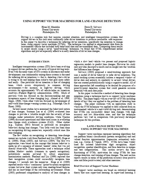
USING SUPPORT VECTOR MACHINES FOR LANE-CHANGE DETECTIONHiren M. Mandalia Dario D. SalvucciDrexelUniversityDrexel UniversityPhiladelphia, PA Philadelphia, PADriving is a complex task that requires constant attention, and intelligent transportation systems thatsupport drivers in this task must continually infer driver intentions to produce reasonable, safe responses.In this paper we describe a technique for inferring driver intentions, specifically the intention to changelanes, using support vector machines (SVMs). The technique was applied to experimental data from aninstrumented vehicle that included both behavioral data and environmental data. Comparing these resultsto recent results using a novel “mind-tracking” technique, we found that SVMs outperformed earlieralgorithms and proved especially effective in early detection of driver lane changes.INTRODUCTIONIntelligent transportation systems (ITS) have been evolving to support drivers perform the vast array of typical driving tasks. Even with the many types of ITS systems in existence and under development, one commonality among these systems is the need for inferring driver intentions — that is, detecting what a driver is trying to do and helping them achieve that goal more safely and easily. One particular driver intention is that of changing lanes, which occurs ubiquitously in common driving environments — for instance, in highway driving, which accounts for approximately 70% of vehicle miles on American roadways (Federal Highway Administration, 1998). Much of previous work has focused on the decision-making and gap acceptance aspects of lane changing (e.g., Ahmed et al, 1996; Gipps, 1986), while other work has focused on development of real-world lane-change warning systems (e.g., Talmadge, Chu & Riney, 2000).Several recent studies have examined the behavioral nature of lane changes. Suzanne Lee et al. (2004) evaluated lane changes to provide a valuable insight into the severity of lane changes under naturalistic driving conditions, while Tijerina (1999) discussed operational and behavioral issues in evaluating lane change crash avoidance systems (CAS). Other studies (e.g., Tijerina, 2005) focused in particular on eye-glance behaviors during lane changes. Very little work has been done on recognizing driving maneuvers, especially critical ones like lane changing.The few studies on recognizing, or detecting, lane-change maneuvers include work from Pentland and Liu (1999), Kuge et al. (2000), Olsen (2003), and Salvucci (2004). The first two approaches were based on the concept that human behavior is made up of a sequence of internal ‘mental’ states that was not directly observable. These approaches used a technique called hidden Markov models (common in speech recognition), probabilistic models powered by robust expectation-maximization methods. Pentland and Liu (1999) reported that their recognition system could successfully recognize lane changes 1.5 seconds into the maneuver. Kuge et al. (2000) reported results with a “continuous” (point-by-point) recognition system; however, their system only uses steering-based features and has no knowledge of the surrounding environment. Olsen (2003) performed comprehensive analysis of lane changes in which a slow lead vehicle was present and proposed logistic regression models to predict lane changes. However his study only provides descriptive results and an insight into the variables that influence lane changes.Salvucci (2004) proposed a mind-tracking approach that uses a model of driver behavior to infer driver intentions. The mind tracking system essentially isolates a temporal window of driver data and extracts its similarity to several virtual drivers that are created probabilistically using a cognitive model. All of these approaches left something to be desired for purposes of a point-by-point detection system that could generate accurate detection with each data point.In this paper we describe a method of detecting lane change intentions using a technique known as support vector machines (SVMs). The paper begins with an overview of SVMs including details of how they are applied to the problem of detecting lane changes. The paper continues with an application study in which the SVM technique was applied to data collected from an instrumented vehicle in a real-world driving task, demonstrating that SVMs can successfully detect lane changes with high accuracy and low false-alarm rates, and that the technique performs very well in comparison with previously developed techniques for this problem.LANE-CHANGE DETECTIONUSING SUPPORT VECTOR MACHINES Support vector machines represent learning algorithms that can perform binary classification (pattern recognition) and real valued function approximation (regression estimation) tasks (see, e.g., Cortes & Vapnik, 1995). SVMs have been widely used for isolated handwritten digit recognition, object recognition, speaker identification, and face detection in images and text categorization. This section reviews the basic functioning of SVMs, motivation for using SVMs for lane change detection, and training of lane changes. The next section reports results in terms of the prediction accuracy (true positive rates and false positive rates) and other measures.Brief Overview of Support Vector MachinesSupport vector machines are based on statistical learning theory that uses supervised learning. In supervised learning, amachine is trained instead of programmed using a number of training examples of input-output pairs. The objective of training is to learn a function which best describes the relation between the inputs and the outputs. In general, any learning problem in statistical learning theory will lead to a solution of the typeEq (1) where the x i, i = 1,…, l are the input examples, K a certain symmetric positive definite function named kernel, and c i a set of parameters to be determined from the examples. For details on the functioning of SVM, readers are encouraged to refer to (Cortes & Vapnik, 1995). In short, the working of SVM can be described as statistical learning machines that map points of different categories in n-dimensional space into a higher dimensional space where the two categories are more separable. The paradigm tries to find an optimal hyperplane in that high dimensional space that best separates the two categories of points. Figure 1 shows an example of two categories of points separated by a hyperplane. Essentially, the hyperplane is learned by the points that are located closest to the hyperplane which are called ‘support vectors’. There can be more than one support vector on each side of the plane.Figure 1: Points separated by a hyperplane.(Source: )Motivation for using SVMsAssessing driver state is a substantial task, complicated by the various nuances and idiosyncrasies that characterize human behavior. Measurable components indicative of driver state may often reside in some high dimensional feature space (see, e.g., Wipf & Rao, 2003). Researchers have found that SVM have been particularly useful for binary classification problems. SVMs offer a robust and efficient classification approach for the problem of lane change detection because they map the driving data to high dimensional feature space where linear hyperplanes are sufficient to separate two categories of data points. A correct choice of kernel and data representation can lead to good solutions.Issues Relevant to Lane-Change DetectionKernel selection. A key issue in using the learning techniques is the choice of the kernel K in Eq (1). The kernel K(x i, x j) defines a dot product between projections of the two inputs x i and x j, in the feature space, the features been {Φ1(x), Φ2(x),…, ΦN(x} with N the dimensionality of the Reproducing Kernel Hilbert Space (see, e.g., Cortes & Vapnik, 1995). Therefore the choice is closely related to the choice of the “effective” representation of the data, e.g. the image representation in a vision application. The problem of choosing the kernel for the SVM, and more generally the issue of finding appropriate data representations for learning, is an important one (e.g., Evgeniou, Pontil, & Poggio, 2000). The theory does not provide a general method for finding “good” data representations, but suggests representations that lead to simple solutions. Although there is no general solution to this problem, several experimental and theoretical works provides insights for specific applications (see, e.g., Evgeniou, Pontil, & Poggio, 2000; Vapnik, 1998). However recent work from researchers (e.g., Lanckriet et al., 2004) has shown that for a given data representation there is a systematic method for kernel estimation using semi-definite programming. Estimating the right kind of kernel remains an important segment of the future work with this kind of work. At this point of time the available data was tested against different types of kernel functions to know the performance of each of them experimentally. Some of the kernel-types tested were Linear, Polynomial, Exponential and Gaussian. However, it was observed that all the kernels performed as good as or worse than Linear kernel. All the final results with SVM classification are therefore analyzed with Linear kernel.Choosing a time window. One issue with using SVM for lane change detection is that lane changes do not have fixed time length. Thus, longer lane changes see a smooth transition in feature values like steering angle, lane position, acceleration, etc. whereas shorter ones have a relatively abrupt transition. Moreover, one feature may be a function of one or many other features. The exact inter-dependency between features or within features themselves is often unclear. In the domain of detecting driving maneuvers like lane changes, the change in the features with respect to time and their inter-dependency is more critical than the individual values of the features. For example, studies have shown that during a lane change drivers exhibit an expected sine-wave steering pattern except for a longer and flatter second peak as they straightened the vehicle (e.g., Salvucci & Liu, 2002). The figure below shows such a pattern of steering against time.Drivers first steer toward the destination and then back to center to level the vehicle on a steady path to the destination lane. Then, in a continual smooth movement, drivers steer in the other direction and back to center to straighten the vehicle.Figure 2: Steering angle displays a sine-wave like pattern(Source: Salvucci & Liu, 2002)Such patterns can only be observed (by humans) or learned (by machines) when a reasonable sized window of samples is observed. Thus for all practical purposes when using the SVM for a lane change or lane keeping, an entire window of samples is input instead of a single sample. A ‘sample’ refers to the set of values of features at that instance of time. The data stream is broken down into fixed-size smaller windows. The size (time length) of the window that adequately captures the patterns within the features is a free parameter and therefore left to experimentation. Various window sizes were analyzed between 1 second to 5 seconds. The results with different window sizes are reported in the results. About 2/3rd of driving data was used for training SVMs and remaining 1/3rd for testing purposes.Another issue in training is assigning the correct label (LC or LK) to each window. The lane change definition used to classify training data was that a lane change starts when the vehicle moves towards the other lane boundary and never returns i.e. the final shift of the driver towards the other lane. Any reversal cancels the lane change. Using the definition of lane change, each sample within a window can be labeled positive (LC) or negative (LK) but not the entire window. The last sample within the window is used to label the entire window, since the last sample offers the latest information about the driving state. Also in order to predict the driving state at any time only the preceding samples can be used.Figure 3: Moving window of constant sizeAs shown in Figure 3 a single window of size N is defined by N samples at times {t 0, t 1,…, t N-1}. The label of sample at t N-1 is assigned to the entire window. A moving window is used as shown in the figure i.e. whenever a new sample is obtained, it is added to the moving window and the last sample is dropped, maintaining a constant size window.Choosing a data representation . The general problem of finding an optimal, or even reasonable, data representation is an open one. One approach to data representation is to input the entire training window to the SVM with the actual values of thefeatures (e.g., Wipf & Rao, 2003) and feed them to Relevance Vector Machines (RVM). In such an approach, an input vector corresponding to a single window of size N samples looks like[steerangle(t 0),…,steerangle(t N-1),speed(t 0),…,speed(t N-1),…]which in general is equivalent to[F 1(t 0),…,F 1(t N-1), F 2(t 0),…,F 2(t N-1),…,F M (t 0),…,F M (t N-1)]where F x (t i ) represents the value of feature F x at time t i . Such a vector is used to train Relevance Vector Machines (RVM). RVM is a probabilistic sparse kernel model identical in functional form to the SVM (e.g., Cortes & Vapnik, 1995).Embedded in this formulation is the fact that temporal variations in maneuver execution are handled implicitly by RVMs. However, inherent functionalities of RVMs or SVMs would fail to observe any dependencies or relationship between values of a feature over a period of time which could be critical. Also this formulation results in abnormally long sized input vector leading to additional computational complexity.An alternative approach is suggested to explicitly include some form of dependency/relationship measure between feature values rather than the original values. As argued previously it is the change pattern in the feature values which is more critical than the values themselves. Variance of a feature over all the samples in the block was used to replace the original values of that feature. Variance of a feature is given byEq (2)where N is the window size (number of samples), µx is the mean of the feature F x within the window and x i is the feature value of the i th sample. Thus variance effectively captures the change in the feature values which is very critical to learn specific patterns. Variance of features is particularly useful in reducing the effects of noise in the data. Another reason that encouraged the use of variance is the reduced size of input vectors that were used for final training as explained in the following section.Figure 4 explains the two data representations that were experimented using variance. A single window of size N is shown on the left hand side of the two representations where each feature F x has N values. In Data Representation I (non-overlapping), a single window is divided into two equal halves and the variance of features from each half is used. Thus for every N values of a feature only two values of variances from the first and second half of the window contributes to the input vector. The rationale for splitting a single window in two halves is the need to capture multiple change patterns within a window. For example, features like lane position or steer angle might change multiple times within a window but a single variance across the window will reflect only the overall change.Data Representation II (overlapping) shown in the figure uses a similar structure with the difference that the two halvesFigure 4: Data Representationoverlap with each other. A window of size N is divided into three equal parts say a, b, c. The first half will consist of the first two parts (a, b) and the second half will consist of last two parts. Overlapping structure was tested to account for the fact that the division of a lane change may not be equal and the changes may also happen in the middle of the window. Experiments were performed with each representation.Choosing a feature set. While training the SVMs it is very important that only the most effective set of features, rather than set of all possible features, is used. Features that display significant differences during a lane change against normal driving are the critical ones. Features that do not show enough predictability and vary randomly irrespective of a lane change should be avoided as they degrade the discrimination power of SVM.With no prior preference to any feature, initial experiments included all features. Later, only selected combinations were employed to choose the minimal feature set that would produce the best classification. Various combinations of features were tested. However, only few selected combinations generated good results. Best classification results were obtained with only four features with lane positions at different distances. Such an outcome was expected since lane position demonstrated the most consistent pattern among all the other features. One can argue that steering angle should also be a strong candidate. However, steering angle displays similar patterns both during lane change and while driving through a curved road which led to high number of false positives.Time to collision (TTC) (see, e.g., Olsen, 2003) could be an important feature however; the available data did not have speed values of the lead vehicles. Another limitation was the lack of eye movement data which could prove critical for lane change detection (see, e.g., Olsen, 2003). The current method of feature selection is based purely on experiments. However, as a future study use of more systematic stochastic techniques like t-tests, recursive feature elimination, and maximum likelihood test are planned.The feature sets in Table 1 were selected such that it includes different combinations of features that would generate significant patterns in their variances. Set 1 contains the most basic relevant features. Set 2 measures the effect of lead car distance. Set 3 includes longitudinal and latitudinal information of the car while Set 4 measures the significance of steering angle. Set 5 contains only lane position values since experiments indicated that they were most significant. Note that the lane position features indicate the longitudinal distance from the driver’s vehicle in m — e.g., “Lane position 30” represents the lane position for the point 30 m directly ahead of the vehicle.Generating continuous recognition. To simulate a continuous recognition scheme we use a moving window of size N (block-size) as shown in Figure 3. The window is slided one sample at a time across the data. The classification label predicted by SVM for each window is used as label for the last sample in the window. Consistency among classification scores is one important advantage of this scheme. That is if the previous and next few samples are classified positive the probability of the current sample to be classified negative is very low.Table 1: Feature setsSet Features1 Acceleration, Lane position 0, Lane position 30,Heading2 Acceleration, Lane position 0, Lane position 30,Heading, Lead Car distance3 Acceleration, Lane position 0, Lane Position 20,Lane position 30, Heading, Longitudinalacceleration, Lateral acceleration4 Acceleration, Lane position 0, Lane position 30,Heading, Steering Angle5 Lane position 0, Lane position 10, Lane position 20,Lane position 30EVALUATION STUDYWe performed an evaluation study applying the SVM technique to lane-change detection and, at the same time, exploring a subset of the space of possible data representations and feature sets. For this study, we used the real-world data set collected by T. Yamamura and N. Kuge at Nissan Research Center in Oppama, Japan (see Salvucci, Mandalia, Kuge, & Yamamura, in preparation). Four driver subjects were asked to drive on a Japanese multi-lane highway environment for one hour each through dense and smooth traffic. The drivers were given no specific goals or instructions and they were allowed to drive on their own.The results for the various combinations of window size, feature sets, and non-overlapping vs. overlapping representations are shown in Tables 2 and 3. Average true positive rate at 5% false alarm rate1 among all feature sets is very high, and results improve with decrease in window size. The overlapping representation with all the lane position features (Set 5) generates the best recognition result with 97.9% accuracy2. The system generates a continuous recognition which means it marks each sample with a positive (LC) or negative (LK) label. Thus out of every 100 actual lane-changing samples about 98 are detected correctly, whereas out of every 100 lane-keeping samples only 5 are incorrectly predicted.The recognition system was also analyzed for accuracy with respect to time to calculate how much time is elapsed from the start of a lane change until the point of detection. The system was able to detect about 87% of all true positives within the first 0.3 seconds from the start of the maneuver.DISCUSSIONThe SVM approach to detecting lane changes worked well with real-world vehicle data. A richer data set with features like lead-car velocity, eye movements should lead to even better1 False alarm rate = No. of False Positives * 100 / Total No. of Negatives (LK samples)2 Accuracy = No. of True Positives * 100 / Total No. of Positives (LC samples)accuracy. Comparing the results to previous algorithms, Pentland and Liu (1999) achieved accuracy of 95%, but only after 1.5 seconds into the maneuver whereas our system classifies all data points from the start of the maneuver with 97.9% accuracy. Kuge et al. (2000) achieved 98% accuracy of recognizing entire lane changes (as opposed to point-by-point accuracy). Salvucci’s (2004) results are more directly comparable: his mind-tracking algorithm achieved approximately 87% accuracy at 5% false alarm rate. Thus, the SVM approach outperforms previous approaches and offers great promise as a lane-change detection algorithm for intelligent transportation systems.Table 2: Accuracy by window size (non-overlapping) Window Set 1 Set 2 Set 3 Set 4 Set 5 5s 83.5 90.0 91.2 90.0 91.14s 88.1 91.3 92.5 91.5 92.22s 89.3 93.0 97.7 94.0 97.41.5s 85.2 93.7 96.3 93.2 97.71.2s 96.8 96.0 96.0 96.0 96.70.8s 86.3 91.8 90.0 86.6 94.6Table 3: Accuracy by window size (overlapping) Window Set 1 Set 2 Set 3 Set 4 Set 5 5s 87.1 86.9 89.0 88.1 87.84s 89.9 90.7 91.5 89.5 91.12s 96.2 96.2 97.8 95.8 97.31.5s 94.5 94.6 97.6 93.3 97.51.2s 93.8 93.7 95.0 93.2 97.90.8s 97.0 95.5 96.0 96.4 96.7ACKNOWLEDGMENTSThis work was supported by National Science Foundation grant#IIS-0133083.REFERENCESAhmed, K. I., Ben-Akiva, M. E., Koutsopoulos, H. N., & Mishalani, R. G. (1996). Models of freeway lane changingand gap acceptance behavior. In J.-B. Lesort (Ed.), Transportation and Traffic Theory. New York: Elsevier. Cortes, C. and Vapnik, V. (1995). Support vector networks. Machine Learning, 20:273-295.Evgeniou, T., Pontil, M., & Poggio, T. (2000). Statistical Learning Theory: A Primer. International Journal ofComputer Vision, 38, 9-13.Federal Highway Administration (1998). Our nation’s highways: Selected facts and figures (Tech. Rep. No. FHWA-PL-00-014). Washington, DC: U.S. Dept. of Transportation. Gipps, P. G. (1986). A model for the structure of lane-changing decisions. Transportation Research – Part B, 5, 403-414. Kuge, N., Yamamura, T. and Shimoyama, O. (2000). A Driver Behavior Recognition Method Based on a Driver Model Framework. Intelligent Vehicle Systems (SP-1538). Lanckriet, G. R. G., Cristianini, N., Barlett, P., Ghaoui, L. E., & Jordan, M. I. (2004). Learning the Kernel Matrix with Semidefinite Programming. Journal of Machine Learning Research 5, pp. 27-72.Lee, S. E., Olsen, E. C. B., & Wierwille, W. W. (2004). Naturalistic lane change field data reduction, analysis, and archiving: A comprehensive examination of naturalistic lane-changes (Tech. Rep. No. DOT-HS-809-702). National Highway Traffic Safety Administration.Olsen, E. C. B., (2003). Modeling slow lead vehicle lane changing. Doctoral Dissertation, Department of Industrial and Systems Engineering, Virginia Polytechnic Institute. Pentland, A., & Liu, A. (1999). Modeling and prediction of human behavior. Neural Computation, 11, 229-242. Salvucci, D. D. (2004). Inferring driver intent: A case study in lane-change detection. In Proceedings of the Human Factors Ergonomics Society 48th Annual Meeting.Salvucci, D. D., & Liu, A. (2002). The time course of a lane change: Driver control and eye-movement behavior. Transportation Research Part F, 5, 123-132.Salvucci, D.D., Mandalia, H.M., Kuge, N., & Yamamura, T. (in preparation). Comparing lane-change detection algorithms on driving-simulator and instrumented-vehicle data. In preparation for submission to Human Factors. Talmadge, S., Chu, R. Y., & Riney, R. S. (2000). Description and preliminary data from TRW’s lane change collision avoidance testbed. In Proceedings of the Intelligent Transportation Society of America’s Tenth Annual Meeting. Tijerina, L. (1999). Operational and behavioral issues in the comprehensive evaluation of lane change crash avoidance systems. J. of Transportation Human Factors, 1, 159-176. Tijerina, L., Garott W. R., Stoltzfus, D., Parmer, E., (2005). Van and Passenger Car Driver Eye Glance Behavior During the Lane Change Decision Phase. In Proceedings of Transportation Research Board Annual Meeting 2005. Vapnik, V.N. (1998). Statistical Learning Theory. Wiley: NY. Wipf, D. & Rao, B. (2003). Driver Intent Inference Annual Report, University of California, San Diego.。
基于Codebook背景建模的视频行人检测
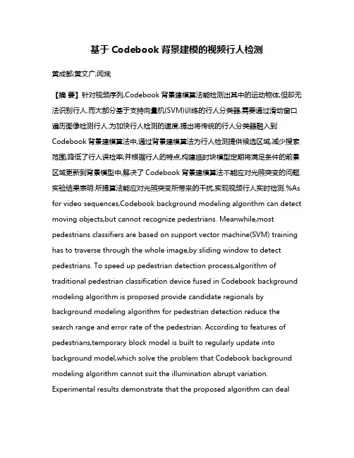
基于Codebook背景建模的视频行人检测黄成都;黄文广;闫斌【摘要】针对视频序列,Codebook背景建模算法能检测出其中的运动物体,但却无法识别行人.而大部分基于支持向量机(SVM)训练的行人分类器,需要通过滑动窗口遍历图像检测行人.为加快行人检测的速度,提出将传统的行人分类器融入到Codebook背景建模算法中,通过背景建模算法为行人检测提供候选区域,减少搜索范围,降低了行人误检率;并根据行人的特点,构建临时块模型定期将满足条件的前景区域更新到背景模型中,解决了Codebook背景建模算法不能应对光照突变的问题.实验结果表明:所提算法能应对光照突变所带来的干扰,实现视频行人实时检测.%As for video sequences,Codebook background modeling algorithm can detect moving objects,but cannot recognize pedestrians. Meanwhile,most pedestrians classifiers are based on support vector machine(SVM) training has to traverse through the whole image,by sliding window to detect pedestrians. To speed up pedestrian detection process,algorithm of traditional pedestrian classification device fused in Codebook background modeling algorithm is proposed provide candidate regionals by background modeling algorithm for pedestrian detection reduce the search range and error rate of the pedestrian. According to features of pedestrians,temporary block model is built to regularly update into background model,which solve the problem that Codebook background modeling algorithm cannot suit the illumination abrupt variation. Experimental results demonstrate that the proposed algorithm can dealwith the interference caused by sudden light variation,it can achieve the real-time pedestrian detection in video.【期刊名称】《传感器与微系统》【年(卷),期】2017(036)003【总页数】3页(P144-146)【关键词】视频;Codebook背景建模;支持向量机;行人检测【作者】黄成都;黄文广;闫斌【作者单位】电子科技大学自动化工程学院,四川成都611731;国家电网四川省电力公司乐山电业局,四川乐山614000;电子科技大学自动化工程学院,四川成都611731【正文语种】中文【中图分类】TP391.4行人检测对于一个智能监控系统至关重要,是异常行为识别[1,2]、行人识别与跟踪[3]、步态识别[4,5]、行人计数[6,7]等智能应用的基础。
Support vector machine_A tool for mapping mineral prospectivity
Support vector machine:A tool for mapping mineral prospectivityRenguang Zuo a,n,Emmanuel John M.Carranza ba State Key Laboratory of Geological Processes and Mineral Resources,China University of Geosciences,Wuhan430074;Beijing100083,Chinab Department of Earth Systems Analysis,Faculty of Geo-Information Science and Earth Observation(ITC),University of Twente,Enschede,The Netherlandsa r t i c l e i n f oArticle history:Received17May2010Received in revised form3September2010Accepted25September2010Keywords:Supervised learning algorithmsKernel functionsWeights-of-evidenceTurbidite-hosted AuMeguma Terraina b s t r a c tIn this contribution,we describe an application of support vector machine(SVM),a supervised learningalgorithm,to mineral prospectivity mapping.The free R package e1071is used to construct a SVM withsigmoid kernel function to map prospectivity for Au deposits in western Meguma Terrain of Nova Scotia(Canada).The SVM classification accuracies of‘deposit’are100%,and the SVM classification accuracies ofthe‘non-deposit’are greater than85%.The SVM classifications of mineral prospectivity have5–9%lowertotal errors,13–14%higher false-positive errors and25–30%lower false-negative errors compared tothose of the WofE prediction.The prospective target areas predicted by both SVM and WofE reflect,nonetheless,controls of Au deposit occurrence in the study area by NE–SW trending anticlines andcontact zones between Goldenville and Halifax Formations.The results of the study indicate theusefulness of SVM as a tool for predictive mapping of mineral prospectivity.&2010Elsevier Ltd.All rights reserved.1.IntroductionMapping of mineral prospectivity is crucial in mineral resourcesexploration and mining.It involves integration of information fromdiverse geoscience datasets including geological data(e.g.,geologicalmap),geochemical data(e.g.,stream sediment geochemical data),geophysical data(e.g.,magnetic data)and remote sensing data(e.g.,multispectral satellite data).These sorts of data can be visualized,processed and analyzed with the support of computer and GIStechniques.Geocomputational techniques for mapping mineral pro-spectivity include weights of evidence(WofE)(Bonham-Carter et al.,1989),fuzzy WofE(Cheng and Agterberg,1999),logistic regression(Agterberg and Bonham-Carter,1999),fuzzy logic(FL)(Ping et al.,1991),evidential belief functions(EBF)(An et al.,1992;Carranza andHale,2003;Carranza et al.,2005),neural networks(NN)(Singer andKouda,1996;Porwal et al.,2003,2004),a‘wildcat’method(Carranza,2008,2010;Carranza and Hale,2002)and a hybrid method(e.g.,Porwalet al.,2006;Zuo et al.,2009).These techniques have been developed toquantify indices of occurrence of mineral deposit occurrence byintegrating multiple evidence layers.Some geocomputational techni-ques can be performed using popular software packages,such asArcWofE(a free ArcView extension)(Kemp et al.,1999),ArcSDM9.3(afree ArcGIS9.3extension)(Sawatzky et al.,2009),MI-SDM2.50(aMapInfo extension)(Avantra Geosystems,2006),GeoDAS(developedbased on MapObjects,which is an Environmental Research InstituteDevelopment Kit)(Cheng,2000).Other geocomputational techniques(e.g.,FL and NN)can be performed by using R and Matlab.Geocomputational techniques for mineral prospectivity map-ping can be categorized generally into two types–knowledge-driven and data-driven–according to the type of inferencemechanism considered(Bonham-Carter1994;Pan and Harris2000;Carranza2008).Knowledge-driven techniques,such as thosethat apply FL and EBF,are based on expert knowledge andexperience about spatial associations between mineral prospec-tivity criteria and mineral deposits of the type sought.On the otherhand,data-driven techniques,such as WofE and NN,are based onthe quantification of spatial associations between mineral pro-spectivity criteria and known occurrences of mineral deposits ofthe type sought.Additional,the mixing of knowledge-driven anddata-driven methods also is used for mapping of mineral prospec-tivity(e.g.,Porwal et al.,2006;Zuo et al.,2009).Every geocomputa-tional technique has advantages and disadvantages,and one or theother may be more appropriate for a given geologic environmentand exploration scenario(Harris et al.,2001).For example,one ofthe advantages of WofE is its simplicity,and straightforwardinterpretation of the weights(Pan and Harris,2000),but thismodel ignores the effects of possible correlations amongst inputpredictor patterns,which generally leads to biased prospectivitymaps by assuming conditional independence(Porwal et al.,2010).Comparisons between WofE and NN,NN and LR,WofE,NN and LRfor mineral prospectivity mapping can be found in Singer andKouda(1999),Harris and Pan(1999)and Harris et al.(2003),respectively.Mapping of mineral prospectivity is a classification process,because its product(i.e.,index of mineral deposit occurrence)forevery location is classified as either prospective or non-prospectiveaccording to certain combinations of weighted mineral prospec-tivity criteria.There are two types of classification techniques.Contents lists available at ScienceDirectjournal homepage:/locate/cageoComputers&Geosciences0098-3004/$-see front matter&2010Elsevier Ltd.All rights reserved.doi:10.1016/j.cageo.2010.09.014n Corresponding author.E-mail addresses:zrguang@,zrguang1981@(R.Zuo).Computers&Geosciences](]]]])]]]–]]]One type is known as supervised classification,which classifies mineral prospectivity of every location based on a training set of locations of known deposits and non-deposits and a set of evidential data layers.The other type is known as unsupervised classification, which classifies mineral prospectivity of every location based solely on feature statistics of individual evidential data layers.A support vector machine(SVM)is a model of algorithms for supervised classification(Vapnik,1995).Certain types of SVMs have been developed and applied successfully to text categorization, handwriting recognition,gene-function prediction,remote sensing classification and other studies(e.g.,Joachims1998;Huang et al.,2002;Cristianini and Scholkopf,2002;Guo et al.,2005; Kavzoglu and Colkesen,2009).An SVM performs classification by constructing an n-dimensional hyperplane in feature space that optimally separates evidential data of a predictor variable into two categories.In the parlance of SVM literature,a predictor variable is called an attribute whereas a transformed attribute that is used to define the hyperplane is called a feature.The task of choosing the most suitable representation of the target variable(e.g.,mineral prospectivity)is known as feature selection.A set of features that describes one case(i.e.,a row of predictor values)is called a feature vector.The feature vectors near the hyperplane are the support feature vectors.The goal of SVM modeling is tofind the optimal hyperplane that separates clusters of feature vectors in such a way that feature vectors representing one category of the target variable (e.g.,prospective)are on one side of the plane and feature vectors representing the other category of the target variable(e.g.,non-prospective)are on the other size of the plane.A good separation is achieved by the hyperplane that has the largest distance to the neighboring data points of both categories,since in general the larger the margin the better the generalization error of the classifier.In this paper,SVM is demonstrated as an alternative tool for integrating multiple evidential variables to map mineral prospectivity.2.Support vector machine algorithmsSupport vector machines are supervised learning algorithms, which are considered as heuristic algorithms,based on statistical learning theory(Vapnik,1995).The classical task of a SVM is binary (two-class)classification.Suppose we have a training set composed of l feature vectors x i A R n,where i(¼1,2,y,n)is the number of feature vectors in training samples.The class in which each sample is identified to belong is labeled y i,which is equal to1for one class or is equal toÀ1for the other class(i.e.y i A{À1,1})(Huang et al., 2002).If the two classes are linearly separable,then there exists a family of linear separators,also called separating hyperplanes, which satisfy the following set of equations(KavzogluandFig.1.Support vectors and optimum hyperplane for the binary case of linearly separable data sets.Table1Experimental data.yer A Layer B Layer C Layer D Target yer A Layer B Layer C Layer D Target1111112100000 2111112200000 3111112300000 4111112401000 5111112510000 6111112600000 7111112711100 8111112800000 9111012900000 10111013000000 11101113111100 12111013200000 13111013300000 14111013400000 15011013510000 16101013600000 17011013700000 18010113811100 19010112900000 20101014010000R.Zuo,E.J.M.Carranza/Computers&Geosciences](]]]])]]]–]]]2Colkesen,2009)(Fig.1):wx iþb Zþ1for y i¼þ1wx iþb rÀ1for y i¼À1ð1Þwhich is equivalent toy iðwx iþbÞZ1,i¼1,2,...,nð2ÞThe separating hyperplane can then be formalized as a decision functionfðxÞ¼sgnðwxþbÞð3Þwhere,sgn is a sign function,which is defined as follows:sgnðxÞ¼1,if x400,if x¼0À1,if x o08><>:ð4ÞThe two parameters of the separating hyperplane decision func-tion,w and b,can be obtained by solving the following optimization function:Minimize tðwÞ¼12J w J2ð5Þsubject toy Iððwx iÞþbÞZ1,i¼1,...,lð6ÞThe solution to this optimization problem is the saddle point of the Lagrange functionLðw,b,aÞ¼1J w J2ÀX li¼1a iðy iððx i wÞþbÞÀ1Þð7Þ@ @b Lðw,b,aÞ¼0@@wLðw,b,aÞ¼0ð8Þwhere a i is a Lagrange multiplier.The Lagrange function is minimized with respect to w and b and is maximized with respect to a grange multipliers a i are determined by the following optimization function:MaximizeX li¼1a iÀ12X li,j¼1a i a j y i y jðx i x jÞð9Þsubject toa i Z0,i¼1,...,l,andX li¼1a i y i¼0ð10ÞThe separating rule,based on the optimal hyperplane,is the following decision function:fðxÞ¼sgnX li¼1y i a iðxx iÞþb!ð11ÞMore details about SVM algorithms can be found in Vapnik(1995) and Tax and Duin(1999).3.Experiments with kernel functionsFor spatial geocomputational analysis of mineral exploration targets,the decision function in Eq.(3)is a kernel function.The choice of a kernel function(K)and its parameters for an SVM are crucial for obtaining good results.The kernel function can be usedTable2Errors of SVM classification using linear kernel functions.l Number ofsupportvectors Testingerror(non-deposit)(%)Testingerror(deposit)(%)Total error(%)0.2580.00.00.0180.00.00.0 1080.00.00.0 10080.00.00.0 100080.00.00.0Table3Errors of SVM classification using polynomial kernel functions when d¼3and r¼0. l Number ofsupportvectorsTestingerror(non-deposit)(%)Testingerror(deposit)(%)Total error(%)0.25120.00.00.0160.00.00.01060.00.00.010060.00.00.0 100060.00.00.0Table4Errors of SVM classification using polynomial kernel functions when l¼0.25,r¼0.d Number ofsupportvectorsTestingerror(non-deposit)(%)Testingerror(deposit)(%)Total error(%)11110.00.0 5.010290.00.00.0100230.045.022.5 1000200.090.045.0Table5Errors of SVM classification using polynomial kernel functions when l¼0.25and d¼3.r Number ofsupportvectorsTestingerror(non-deposit)(%)Testingerror(deposit)(%)Total error(%)0120.00.00.01100.00.00.01080.00.00.010080.00.00.0 100080.00.00.0Table6Errors of SVM classification using radial kernel functions.l Number ofsupportvectorsTestingerror(non-deposit)(%)Testingerror(deposit)(%)Total error(%)0.25140.00.00.01130.00.00.010130.00.00.0100130.00.00.0 1000130.00.00.0Table7Errors of SVM classification using sigmoid kernel functions when r¼0.l Number ofsupportvectorsTestingerror(non-deposit)(%)Testingerror(deposit)(%)Total error(%)0.25400.00.00.01400.035.017.510400.0 6.0 3.0100400.0 6.0 3.0 1000400.0 6.0 3.0R.Zuo,E.J.M.Carranza/Computers&Geosciences](]]]])]]]–]]]3to construct a non-linear decision boundary and to avoid expensive calculation of dot products in high-dimensional feature space.The four popular kernel functions are as follows:Linear:Kðx i,x jÞ¼l x i x j Polynomial of degree d:Kðx i,x jÞ¼ðl x i x jþrÞd,l40Radial basis functionðRBFÞ:Kðx i,x jÞ¼exp fÀl99x iÀx j992g,l40 Sigmoid:Kðx i,x jÞ¼tanhðl x i x jþrÞ,l40ð12ÞThe parameters l,r and d are referred to as kernel parameters. The parameter l serves as an inner product coefficient in the polynomial function.In the case of the RBF kernel(Eq.(12)),l determines the RBF width.In the sigmoid kernel,l serves as an inner product coefficient in the hyperbolic tangent function.The parameter r is used for kernels of polynomial and sigmoid types. The parameter d is the degree of a polynomial function.We performed some experiments to explore the performance of the parameters used in a kernel function.The dataset used in the experiments(Table1),which are derived from the study area(see below),were compiled according to the requirementfor Fig.2.Simplified geological map in western Meguma Terrain of Nova Scotia,Canada(after,Chatterjee1983;Cheng,2008).Table8Errors of SVM classification using sigmoid kernel functions when l¼0.25.r Number ofSupportVectorsTestingerror(non-deposit)(%)Testingerror(deposit)(%)Total error(%)0400.00.00.01400.00.00.010400.00.00.0100400.00.00.01000400.00.00.0R.Zuo,E.J.M.Carranza/Computers&Geosciences](]]]])]]]–]]]4classification analysis.The e1071(Dimitriadou et al.,2010),a freeware R package,was used to construct a SVM.In e1071,the default values of l,r and d are1/(number of variables),0and3,respectively.From the study area,we used40geological feature vectors of four geoscience variables and a target variable for classification of mineral prospec-tivity(Table1).The target feature vector is either the‘non-deposit’class(or0)or the‘deposit’class(or1)representing whether mineral exploration target is absent or present,respectively.For‘deposit’locations,we used the20known Au deposits.For‘non-deposit’locations,we randomly selected them according to the following four criteria(Carranza et al.,2008):(i)non-deposit locations,in contrast to deposit locations,which tend to cluster and are thus non-random, must be random so that multivariate spatial data signatures are highly non-coherent;(ii)random non-deposit locations should be distal to any deposit location,because non-deposit locations proximal to deposit locations are likely to have similar multivariate spatial data signatures as the deposit locations and thus preclude achievement of desired results;(iii)distal and random non-deposit locations must have values for all the univariate geoscience spatial data;(iv)the number of distal and random non-deposit locations must be equaltoFig.3.Evidence layers used in mapping prospectivity for Au deposits(from Cheng,2008):(a)and(b)represent optimum proximity to anticline axes(2.5km)and contacts between Goldenville and Halifax formations(4km),respectively;(c)and(d)represent,respectively,background and anomaly maps obtained via S-Afiltering of thefirst principal component of As,Cu,Pb and Zn data.R.Zuo,E.J.M.Carranza/Computers&Geosciences](]]]])]]]–]]]5the number of deposit locations.We used point pattern analysis (Diggle,1983;2003;Boots and Getis,1988)to evaluate degrees of spatial randomness of sets of non-deposit locations and tofind distance from any deposit location and corresponding probability that one deposit location is situated next to another deposit location.In the study area,we found that the farthest distance between pairs of Au deposits is71km,indicating that within that distance from any deposit location in there is100%probability of another deposit location. However,few non-deposit locations can be selected beyond71km of the individual Au deposits in the study area.Instead,we selected random non-deposit locations beyond11km from any deposit location because within this distance from any deposit location there is90% probability of another deposit location.When using a linear kernel function and varying l from0.25to 1000,the number of support vectors and the testing errors for both ‘deposit’and‘non-deposit’do not vary(Table2).In this experiment the total error of classification is0.0%,indicating that the accuracy of classification is not sensitive to the choice of l.With a polynomial kernel function,we tested different values of l, d and r as follows.If d¼3,r¼0and l is increased from0.25to1000,the number of support vectors decreases from12to6,but the testing errors for‘deposit’and‘non-deposit’remain nil(Table3).If l¼0.25, r¼0and d is increased from1to1000,the number of support vectors firstly increases from11to29,then decreases from23to20,the testing error for‘non-deposit’decreases from10.0%to0.0%,whereas the testing error for‘deposit’increases from0.0%to90%(Table4). In this experiment,the total error of classification is minimum(0.0%) when d¼10(Table4).If l¼0.25,d¼3and r is increased from 0to1000,the number of support vectors decreases from12to8,but the testing errors for‘deposit’and‘non-deposit’remain nil(Table5).When using a radial kernel function and varying l from0.25to 1000,the number of support vectors decreases from14to13,but the testing errors of‘deposit’and‘non-deposit’remain nil(Table6).With a sigmoid kernel function,we experimented with different values of l and r as follows.If r¼0and l is increased from0.25to1000, the number of support vectors is40,the testing errors for‘non-deposit’do not change,but the testing error of‘deposit’increases from 0.0%to35.0%,then decreases to6.0%(Table7).In this experiment,the total error of classification is minimum at0.0%when l¼0.25 (Table7).If l¼0.25and r is increased from0to1000,the numbers of support vectors and the testing errors of‘deposit’and‘non-deposit’do not change and the total error remains nil(Table8).The results of the experiments demonstrate that,for the datasets in the study area,a linear kernel function,a polynomial kernel function with d¼3and r¼0,or l¼0.25,r¼0and d¼10,or l¼0.25and d¼3,a radial kernel function,and a sigmoid kernel function with r¼0and l¼0.25are optimal kernel functions.That is because the testing errors for‘deposit’and‘non-deposit’are0%in the SVM classifications(Tables2–8).Nevertheless,a sigmoid kernel with l¼0.25and r¼0,compared to all the other kernel functions,is the most optimal kernel function because it uses all the input support vectors for either‘deposit’or‘non-deposit’(Table1)and the training and testing errors for‘deposit’and‘non-deposit’are0% in the SVM classification(Tables7and8).4.Prospectivity mapping in the study areaThe study area is located in western Meguma Terrain of Nova Scotia,Canada.It measures about7780km2.The host rock of Au deposits in this area consists of Cambro-Ordovician low-middle grade metamorphosed sedimentary rocks and a suite of Devonian aluminous granitoid intrusions(Sangster,1990;Ryan and Ramsay, 1997).The metamorphosed sedimentary strata of the Meguma Group are the lower sand-dominatedflysch Goldenville Formation and the upper shalyflysch Halifax Formation occurring in the central part of the study area.The igneous rocks occur mostly in the northern part of the study area(Fig.2).In this area,20turbidite-hosted Au deposits and occurrences (Ryan and Ramsay,1997)are found in the Meguma Group, especially near the contact zones between Goldenville and Halifax Formations(Chatterjee,1983).The major Au mineralization-related geological features are the contact zones between Gold-enville and Halifax Formations,NE–SW trending anticline axes and NE–SW trending shear zones(Sangster,1990;Ryan and Ramsay, 1997).This dataset has been used to test many mineral prospec-tivity mapping algorithms(e.g.,Agterberg,1989;Cheng,2008). More details about the geological settings and datasets in this area can be found in Xu and Cheng(2001).We used four evidence layers(Fig.3)derived and used by Cheng (2008)for mapping prospectivity for Au deposits in the yers A and B represent optimum proximity to anticline axes(2.5km) and optimum proximity to contacts between Goldenville and Halifax Formations(4km),yers C and D represent variations in geochemical background and anomaly,respectively, as modeled by multifractalfilter mapping of thefirst principal component of As,Cu,Pb,and Zn data.Details of how the four evidence layers were obtained can be found in Cheng(2008).4.1.Training datasetThe application of SVM requires two subsets of training loca-tions:one training subset of‘deposit’locations representing presence of mineral deposits,and a training subset of‘non-deposit’locations representing absence of mineral deposits.The value of y i is1for‘deposits’andÀ1for‘non-deposits’.For‘deposit’locations, we used the20known Au deposits(the sixth column of Table1).For ‘non-deposit’locations(last column of Table1),we obtained two ‘non-deposit’datasets(Tables9and10)according to the above-described selection criteria(Carranza et al.,2008).We combined the‘deposits’dataset with each of the two‘non-deposit’datasets to obtain two training datasets.Each training dataset commonly contains20known Au deposits but contains different20randomly selected non-deposits(Fig.4).4.2.Application of SVMBy using the software e1071,separate SVMs both with sigmoid kernel with l¼0.25and r¼0were constructed using the twoTable9The value of each evidence layer occurring in‘non-deposit’dataset1.yer A Layer B Layer C Layer D100002000031110400005000061000700008000090100 100100 110000 120000 130000 140000 150000 160100 170000 180000 190100 200000R.Zuo,E.J.M.Carranza/Computers&Geosciences](]]]])]]]–]]] 6training datasets.With training dataset1,the classification accuracies for‘non-deposits’and‘deposits’are95%and100%, respectively;With training dataset2,the classification accuracies for‘non-deposits’and‘deposits’are85%and100%,respectively.The total classification accuracies using the two training datasets are97.5%and92.5%,respectively.The patterns of the predicted prospective target areas for Au deposits(Fig.5)are defined mainly by proximity to NE–SW trending anticlines and proximity to contact zones between Goldenville and Halifax Formations.This indicates that‘geology’is better than‘geochemistry’as evidence of prospectivity for Au deposits in this area.With training dataset1,the predicted prospective target areas occupy32.6%of the study area and contain100%of the known Au deposits(Fig.5a).With training dataset2,the predicted prospec-tive target areas occupy33.3%of the study area and contain95.0% of the known Au deposits(Fig.5b).In contrast,using the same datasets,the prospective target areas predicted via WofE occupy 19.3%of study area and contain70.0%of the known Au deposits (Cheng,2008).The error matrices for two SVM classifications show that the type1(false-positive)and type2(false-negative)errors based on training dataset1(Table11)and training dataset2(Table12)are 32.6%and0%,and33.3%and5%,respectively.The total errors for two SVM classifications are16.3%and19.15%based on training datasets1and2,respectively.In contrast,the type1and type2 errors for the WofE prediction are19.3%and30%(Table13), respectively,and the total error for the WofE prediction is24.65%.The results show that the total errors of the SVM classifications are5–9%lower than the total error of the WofE prediction.The 13–14%higher false-positive errors of the SVM classifications compared to that of the WofE prediction suggest that theSVMFig.4.The locations of‘deposit’and‘non-deposit’.Table10The value of each evidence layer occurring in‘non-deposit’dataset2.yer A Layer B Layer C Layer D110102000030000411105000060110710108000091000101110111000120010131000140000150000161000171000180010190010200000R.Zuo,E.J.M.Carranza/Computers&Geosciences](]]]])]]]–]]]7classifications result in larger prospective areas that may not contain undiscovered deposits.However,the 25–30%higher false-negative error of the WofE prediction compared to those of the SVM classifications suggest that the WofE analysis results in larger non-prospective areas that may contain undiscovered deposits.Certainly,in mineral exploration the intentions are notto miss undiscovered deposits (i.e.,avoid false-negative error)and to minimize exploration cost in areas that may not really contain undiscovered deposits (i.e.,keep false-positive error as low as possible).Thus,results suggest the superiority of the SVM classi-fications over the WofE prediction.5.ConclusionsNowadays,SVMs have become a popular geocomputational tool for spatial analysis.In this paper,we used an SVM algorithm to integrate multiple variables for mineral prospectivity mapping.The results obtained by two SVM applications demonstrate that prospective target areas for Au deposits are defined mainly by proximity to NE–SW trending anticlines and to contact zones between the Goldenville and Halifax Formations.In the study area,the SVM classifications of mineral prospectivity have 5–9%lower total errors,13–14%higher false-positive errors and 25–30%lower false-negative errors compared to those of the WofE prediction.These results indicate that SVM is a potentially useful tool for integrating multiple evidence layers in mineral prospectivity mapping.Table 11Error matrix for SVM classification using training dataset 1.Known All ‘deposits’All ‘non-deposits’TotalPrediction ‘Deposit’10032.6132.6‘Non-deposit’067.467.4Total100100200Type 1(false-positive)error ¼32.6.Type 2(false-negative)error ¼0.Total error ¼16.3.Note :Values in the matrix are percentages of ‘deposit’and ‘non-deposit’locations.Table 12Error matrix for SVM classification using training dataset 2.Known All ‘deposits’All ‘non-deposits’TotalPrediction ‘Deposits’9533.3128.3‘Non-deposits’566.771.4Total100100200Type 1(false-positive)error ¼33.3.Type 2(false-negative)error ¼5.Total error ¼19.15.Note :Values in the matrix are percentages of ‘deposit’and ‘non-deposit’locations.Table 13Error matrix for WofE prediction.Known All ‘deposits’All ‘non-deposits’TotalPrediction ‘Deposit’7019.389.3‘Non-deposit’3080.7110.7Total100100200Type 1(false-positive)error ¼19.3.Type 2(false-negative)error ¼30.Total error ¼24.65.Note :Values in the matrix are percentages of ‘deposit’and ‘non-deposit’locations.Fig.5.Prospective targets area for Au deposits delineated by SVM.(a)and (b)are obtained using training dataset 1and 2,respectively.R.Zuo,E.J.M.Carranza /Computers &Geosciences ](]]]])]]]–]]]8。
南航大论文写作要求(最新版)

南京航空航天大学研究生学位论文撰写要求(2015年4月修订)一、学位论文的构成学位论文由三部分组成:学位论文前置部分、学位论文主体部分、学位论文附录部分。
二、各部分内容的要求1、学位论文前置部分包括封面、承诺书、中英文摘要、目录、图表清单、注释表。
(1) 封面按规定的格式、颜色统一到校印刷厂印制,详见附1。
论文编号:由学校代码,学院编号,年份(后两位),学生类别(S代表硕士,B代表博士)及三位序号组成。
示例:1028701 11-B026(南京航空航天大学航空宇航学院2011年第026号博士学位论文) 分类号:根据论文中主题内容,对照分类法选取中图分类号、学科分类号,著录在左上角。
中图分类号一般选取1~2个,学科分类号标注1个。
中图分类号参照《中国图书资料分类法》、《中国图书馆分类法》,学科分类号参照国务院学位委员会办公室颁布的《学术学位授予信息采集学科代码标准》。
题目:要能概括整个论文最重要的内容,具体、切题、不能太笼统,但要引人注目;题名力求简短,严格控制在25字以内。
学科专业:以国务院学位委员会批准的专业目录中的学科专业为准,填写二级学科名称;申请自主设置二级学科的学位,须填写一级学科名称,并同时填写自主设置二级学科名称,在自主设置二级学科名称上加括号,如力学(纳米力学)。
指导老师:指导老师的署名一律以批准招生的为准,如有变动要正式提出申请并报研究生院备案,且只能写一名指导教师,如有其他正式批准备案的导师,写在联合指导教师一项中(限一名)。
(2) 英文封面(详见附2)(3) 承诺书单设一页,排在英文封面后,请认真阅读承诺书内容,全面审视自己的论文,是否严格遵守《中华人民共和国著作权法》,对他人享有著作权的内容是否都进行了明确的标注,慎重签名。
详见附3。
(4) 中文摘要在论文的第一页,是学位论文内容的不加注释和评论的简短陈述,简要说明研究工作的目的、方法、创新性的成果和结论等。
硕士论文摘要中文字数400~600个字,博士论文摘要中文字数800~1000个字。
基于数字信号处理器的异步电机参数辨识实现
控制与应用技术基于数字信号处理器的异步电机参数辨识实现*刘述喜1, 王明渝2, 陈新岗1, 杨绍荣3, 贺晓蓉1(1.重庆工学院电子信息与自动化学院,重庆 400050;2.重庆大学电气工程学院,重庆 400044;3.重庆三峡水力电力(集团)股份有限公司,重庆 400400)摘 要:介绍了异步电机各种参数的辨识方法。
在不改变硬件系统的前提下,通过电流控制技术,向电机注入单相交流或直流电流,检测其响应,从而实现异步电机的参数辨识。
对一台未知参数的异步电机做仿真和试验研究,并将辨识出来的参数用于矢量控制系统,得到了良好的效果,证明了参数辨识的正确性。
关键词:异步电机;参数辨识;数字信号处理器中图分类号:TM 301.2:TM 343 文献标识码:A 文章编号:1673 6540(2006)10 0021 05I mple m ent of Para m eter Identification ofA synchronousM achineB ased on DSPLIU Shu xi 1, WANG M ing yu 2, C HEN X i n gang 1, Y ANG Shao rong 3, HE X iao rong1(1.Co llege of E lectr on ic I nfor m ation&Auto m ati o n ,Chongq i n g I nstitute ofTec hno l o gy ,Chongqi n g 400050,China ;2.Co llege of E lectrica lEngineeri n g ,Chongqing University ,Chongqi n g 400044,Chi n a ;3.Chongq i n g Three GorgeW ater Conservanly and E lectri c Po wer Co .,Ltd .,Chongqi n g 400400,Chi n a)Abstract :T he sche m e how to esti m a te param eters of asynchronous m ach i ne is introduced .T hen under t he pre m ise o f no chang i ng t he hard w are structure o f vecto r contro l o fm otor ,explaini ng the rea lization of i dentifica ti on of mo tor para m eters t hrough current contro l techno l ogy ,.i e .i nputti ng sing le phase alternati ng current or DC current to the mo tor ,t hen detecti ng t he response .A nd for an unknown para m ete rs mo tor ,the si m ulati on and exper i m ent st udies are perfor m ed ,the i dentified param eters are used to a vector contro l system,be tter effect i s ach i eved wh ich verify i ng the feasi b ilit y o f t he pa rame ters esti m ati on m ethod .K ey word s :asyn chronou s mach i n e ;para m eter identif ication ;digital signal processor*重庆市科委自然科学基金资助项目(C STC 2005BB6076)0 引 言异步电机的矢量控制具有动态性能好、调速范围宽等优点,但不足之处是它的控制性能严重依赖于电机参数的准确性[1]。
飞行术语中英对照整理
Aair superiority 制空权ambush 伏击assistance 援助、协助attitude 飞行姿态(高度)AW ACS(Airborne Warning and Control System) link 空中预警引导aye-aye, sir 遵命,长官(同affirmative)AB 加力ACM 空战机动ACT 空战战术AI 空中拦截Angles 用千英尺表示高度的快捷方式,例如,“Angles 20”表示高度20,000英尺。
Angle-off 敌机航向和你的航向之间的角度差,也称为航向交叉角或HCAArmour star hands 肥厚,笨拙的手,驾驶飞机时容易出错Aspect angle 你的飞机相对于敌机尾部的角度Attack geometry 进攻战机的追击路径Bbail out (爬出座舱)跳伞bearing 航向航向的划分方法是:以飞行员自己的飞机为圆心的一个与地平面平行的虚拟圆,分为360度,正北方为零度,正东方为90度,正南方为180度,正西方为270度,依此类推。
black out 由于指向头部方向的加速度过大而导致的大脑缺血,引起的暂时性失明和意识丧失。
bogie 原指妖怪或可怕的人,空战中指敌机。
bandit 原指强盗,空战中指敌机(同bad guy)bombing run 炸弹攻击brake 阻力板(降落时塔台呼叫call the ball 就是指放下阻力板)bug out 撤出战区bull's eye 原指圆形箭靶的中心,空战中的意思是“正中!”,类似的短语还有:direct hit, great balls of fun, splash one, one down等。
bingo 原指一种赌博游戏或烈酒,空战中指出乎意料地打中了敌机。
只够返回基地的燃料,其它已耗尽的状态。
Bar 雷达波的一次扫描Basic Fighter Maneuvers(BFM)在一对一空战环境中的基本空战机动Belly check 执行180度的翻滚,检查机身下方空间Boresight mode 雷达束固定指向机首前方,第一个进入雷达束区域的目标将被自动锁定Butterfly setup 一个战斗训练进入计划,两架战机开始以一字并列编队飞行,然后互相转离45度。
Fuzzy Support Vector Machines for Pattern Classification
In Section 2, we summarize support vector machines for
pattern classification. And in Section 3 we discuss the problem of the multiclass support vector machines. In Section 4,we discuss the method of defining the membership functions using the SVM decision functions. Finally, in Section 5, we evaluate our method for three benchmark data sets and demonstrate the superiority of the FSVM over the SVM.
two decision functions are positive or all the values are negative. To avoid this, in [3], a pairwise classification method, in which n(n - l ) / 2 decision functions are determined, is proposed. By this method, however unclassifiable regions remain. In this paper, to overcome this problem, we propose fuzzy support vector machines (FSVMs). Using the decision functions obtained by training the SVM, we define truncated polyhedral pyramidal membership functions [4] and resolve unclassifiable regions.
基于支持向量机的数控机床空间误差辨识与补偿(精)
基于支持向量机的数控机床空间误差辨识与补偿)))吴雄彪姚鑫骅何振亚等基于支持向量机的数控机床空间误差辨识与补偿吴雄彪1 姚鑫骅2 何振亚2 傅建中21.金华职业技术学院,金华,3210172.浙江大学,杭州,310027摘要:为了精确地建立数控机床空间误差预测模型,提出基于支持向量机的空间误差辨识与补偿方法。
通过训练学习,优化了最小二乘支持向量机参数,采用激光矢量分步对角线法在一台数控铣床上进行了空间误差辨识和补偿实验研究。
结果表明:支持向量机预测模型能有效辨识数控机床的空间误差。
与神经网络预测模型进行了比较,表明支持向量机空间误差预测模型补偿精度高、建模速度快,通过其补偿可有效提高数控机床的加工精度。
关键词:数控机床;空间误差;支持向量机;误差补偿中图分类号:TG659 文章编号:1004)132X(2010)12)1397)04 IdentificationandCompensationforVolumetricErrorsof CNCMachineToolsBasedonSVM1222WuXiongbiao YaoXinhua HeZhenya FuJianzhong1.JinhuaCollegeofProfessionandTechnology,Jinhua,Zhejiang,3210172.ZhejiangUniversity,Hangzhou,310027Abstract:Anovelmethodofidentificationandcompensationvolumetricerrorsformachinetoo lsbasedonSVMwaspresentedherein.Trainingandlearningtheerrorsamplesandoptimizingth eSVMparameters,thevolumetricerrormodelswereobtainedforcompensation.Bylaserseque ntialstepdiagonalmeasurement,thevolumetricerrorswereidentifiedandcompensated.Thee xperimentalresultsillustratethattheSVMmodelisadaptivetoforecastvolumetricerrorsofma paringtheneutralnetworkmodel,theSVMmodelofvolumetricerrorismorep ingtheSVMvolumetricerrormodel,itissucceededtoenhancetheprecision forCNCmachinetools.Keywords:CNCmachinetool;volumetricerror;supportvectormachine(SVM);errorcompen sation0 引言在数控机床上实现高精度加工的关键是提高机床的空间定位精度。
- 1、下载文档前请自行甄别文档内容的完整性,平台不提供额外的编辑、内容补充、找答案等附加服务。
- 2、"仅部分预览"的文档,不可在线预览部分如存在完整性等问题,可反馈申请退款(可完整预览的文档不适用该条件!)。
- 3、如文档侵犯您的权益,请联系客服反馈,我们会尽快为您处理(人工客服工作时间:9:00-18:30)。
2
3
ABSTterrorist groups that responsible of terrorist attacks is a challenging task and a promising research area. There are many methods that have been developed to address this challenge ranging from supervised to unsupervised methods. The main objective of this research is to conduct a detailed comparative study among Support Vector Machine as one of the successful prediction classifiers that proved highly performance and other supervised machine learning classification and hybrid classification algorithms. Whereas most promising methods are based on support vector machine (SVM); so there is a need for a comprehensive analysis on prediction accuracy of supervised machine learning algorithms on different experimental conditions, and hence in this research we compare predictive accuracy and comprehensibility of explicit, implicit, and hybrid machine learning models and algorithms. This research based on predicting terrorist groups responsible of attacks in Middle East & North Africa from year 2004 up to 2008 by comparing various standard, ensemble, hybrid, and hybrid ensemble machine learning methods and focusing on SVM. The compared classifiers are categorized into main four types namely; Standard Classifiers, Hybrid Classifiers, Ensemble Classifiers, and Hybrid Ensemble Classifiers. In our study we conduct three different experiments on the used real data, afterwards we compare the obtained results according to four different performance measures. Experiments were carried out using real world data represented by Global terrorism Database (GTD) from National Consortium for the study of terrorism and Responses of Terrorism (START).
IPASJ International Journal of Computer Science (IIJCS)
A Publisher for Research Motivation ........
Volume 3, Issue 5, May 2015
Web Site: /IIJCS/IIJCS.htm Email: editoriijcs@ ISSN 2321-5992
1
Department of Operations Research & Decision Support, Faculty of Computers & Information, Cairo University, 5 Dr. Ahmed Zoweil St.- Orman - Postal Code 12613 - Giza – Egypt Department of Operations Research & Decision Support, Faculty of Computers & Information, Cairo University, 5 Dr. Ahmed Zoweil St.- Orman - Postal Code 12613 - Giza – Egypt Department of Operations Research & Decision Support, Faculty of Computers & Information, Cairo University, 5 Dr. Ahmed Zoweil St.- Orman - Postal Code 12613 - Giza – Egypt
Keywords: Hybrid Models, Machine Learning, Predictive Accuracy, Supervised Learning.
1. INTRODUCTION
Machine learning (ML) is the process of estimating unknown dependencies or structures in a system using a limited number of observations [1]. ML algorithms are used in data mining applications to retrieve hidden information. Machine learning methods are rote learning, learning by being told, learning by analogy, and inductive learning, which includes methods of learning by examples and learning by experimentation and discovery [1] [2]. Numerous machine learning methods and different knowledge representation models can be used for predicting different pattern in data set [3]. For example, classification, and regression methods can be used for learning decision trees, rules, Bayes networks, artificial neural networks and support vector machines. Supervised Machine learning classification is one of the tasks most frequently carried out by so called Intelligent Systems. Thus, a large number of techniques have been developed based on Artificial Intelligence (Logic-based techniques, Perceptron-based techniques) and Statistics (Bayesian Networks, Instance-based techniques). The concept of combing classifiers is proposed as a new direction for the improvement of the performance of individual machine learning algorithms. Hybrid and ensemble methods in machine learning have attracted a great attention of the scientific community over the last years [1]. Multiple, ensemble learning models have been theoretically and empirically shown to provide significantly better performance than single weak learners, especially while dealing with high dimensional, complex regression and classification problems [2]. Adaptive hybrid systems has become essential in computational intelligence and soft computing, a main reason for being popular is the high complementary of its components. The integration of the basic technologies into hybrid machine learning solutions [4] facilitate more intelligent search and reasoning methods that match various domain knowledge with empirical data to solve advanced and complex problems [5]. Both ensemble models and hybrid methods make use of the information fusion concept but in slightly different way. In case of ensemble classifiers, multiple but homogeneous, weak models are combined [6], typically at the level of their individual output, using various merging methods, which can be grouped into fixed (e.g., majority voting), and