Jacobi-like Algorithms for Eigenvalue Decomposition of a Real Normal Matrix Using Real Arit
解线性方程组的Jacobi迭代法和投影法之比较
解线性方程组的Jacobi迭代法和投影法之比较
刘长河;刘世祥;寿玉亭
【期刊名称】《北京建筑工程学院学报》
【年(卷),期】2003(019)004
【摘要】从线性方程组的多参数投影法推出Jacobi迭代法.从最优化的观点分析
了Jacobi迭代法收敛速度较慢的原因,即其下降矩阵与步长向量两者并非最优组合.【总页数】3页(P64-66)
【作者】刘长河;刘世祥;寿玉亭
【作者单位】基础部,北京,100044;基础部,北京,100044;基础部,北京,100044
【正文语种】中文
【中图分类】O241.6
【相关文献】
1.在Excel中应用迭代法求解线性方程组——雅可比(Jacobi)和塞德尔(Seidel)迭代法 [J], 杨德祥
2.Jacobi与Gauss-Seidel迭代法求解线性方程组收敛性比较与研究 [J], 王育琳;
贺迅宇;张尚先
3.Jacobi迭代法与Gauss-Seidel迭代法的收敛性比较分析 [J], 白红梅
4.对称正定线性方程组的块Jacobi迭代法的一种改进算法 [J], 徐浩
5.M-矩阵线性方程组的一类Jacobi-Like迭代法 [J], 关晋瑞;宋儒瑛
因版权原因,仅展示原文概要,查看原文内容请购买。
丘赛计算与应用数学考试大纲
丘赛计算与应⽤数学考试⼤纲原⽂地址:Computational MathematicsInterpolation and approximationPolynomial interpolation and least square approximation; trigonometric interpolation and approximation, fast Fourier transform; approximations by rational functions; splines.Nonlinear equation solversConvergence of iterative methods (bisection, secant method, Newton method, other iterative methods) for both scalar equations and systems; finding rootsof polynomials.Linear systems and eigenvalue problemsDirect solvers (Gauss elimination, LU decomposition, pivoting, operation count, banded matrices, round-off error accumulation); iterative solvers (Jacobi, Gauss-Seidel, successive over-relaxation, conjugate gradient method, multi-grid method, Krylov methods); numerical solutions for eigenvalues and eigenvectorsNumerical solutions of ordinary differential equationsOne step methods (Taylor series method and Runge-Kutta method); stability, accuracy and convergence; absolute stability, long time behavior; multi-stepmethodsNumerical solutions of partial differential equationsFinite difference method; stability, accuracy and convergence, Lax equivalence theorem; finite element method, boundary value problemsReferences:[1] C. de Boor and S.D. Conte, Elementary Numerical Analysis, an algorithmicapproach, McGraw-Hill, 2000.[2] G.H. Golub and C.F. van Loan, Matrix Computations, third edition, JohnsHopkins University Press, 1996.[3] E. Hairer, P. Syvert and G. Wanner, Solving Ordinary Differential Equations, Springer, 1993.[4] B. Gustafsson, H.-O. Kreiss and J. Oliger, Time Dependent Problems and Difference Methods, John Wiley Sons, 1995.[5] G. Strang and G. Fix, An Analysis of the Finite Element Method, second edition, Wellesley-Cambridge Press, 2008.Applied MathematicsODE with constant coefficients; Nonlinear ODE: critical points, phase space& stability analysis; Hamiltonian, gradient, conservative ODE's.Calculus of Variations: Euler-Lagrange Equations; Boundary Conditions, parametric formulation; optimal control and Hamiltonian, Pontryagin maximum principle.First order partial differential equations (PDE) and method of characteristics; Heat, wave, and Laplace's equation; Separation of variables and eigen-function expansions; Stationary phase method; Homogenization method for elliptic and linear hyperbolic PDEs; Homogenization and front propagation of Hamil ton-Jacobi equations; Geometric optics for dispersive wave equations. References:W.D. Boyce and R.C. DiPrima, Elementary Differential Equations, Wiley, 2009 F.Y.M. Wan, Introduction to Calculus of Variations and Its Applications, Cha pman & Hall, 1995G. Whitham, "Linear and Nonlinear Waves", John-Wiley and Sons, 1974.J. Keener, "Principles of Applied Mathematics", Addison-Wesley, 1988.A. Benssousan, P-L Lions, G. Papanicolaou, "Asymptotic Analysis for Periodic Structures", North-Holland Publishing Co, 1978.V. Jikov, S. Kozlov, O. Oleinik, "Homogenization of differential operators and integral functions", Springer, 1994.J. Xin, "An Introduction to Fronts in Random Media", Surveys and Tutorials in Applied Math Sciences, No. 5, Springer, 2009。
矩阵雅克比迭代算法
雅克比迭代实验目的:1.学习和掌握线性代数方程组的jacobi 迭代法。
2.运用jacobi 迭代法进行计算。
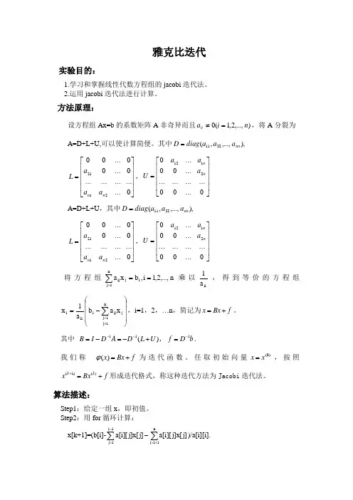
方法原理:设方程组Ax=b 的系数矩阵A 非奇异而且),...,2,1(0n i a ii =≠,将A 分裂为 A=D+L+U,可以使计算简便。
其中),,...,,(2211nn a a a diag D = ⎥⎥⎥⎥⎦⎤⎢⎢⎢⎢⎣⎡=0...............0...00 (002121)n n a a a L ,⎥⎥⎥⎥⎦⎤⎢⎢⎢⎢⎣⎡=0...00...............00...02112n n a a a U A=D+L+U ,其中),,...,,(2211nn a a a diag D =⎥⎥⎥⎥⎦⎤⎢⎢⎢⎢⎣⎡=0...............0...00 (002)121n n a a a L ,⎥⎥⎥⎥⎦⎤⎢⎢⎢⎢⎣⎡=0...00...............00...02112n n a a a U 将方程组n ,...,2,1i ,b x a i n 1j j ij ==∑=乘以ii a 1,得到等价的方程组⎪⎪⎪⎭⎫ ⎝⎛-=∑≠=n i j 1j j ij i ii i x a b a 1x ,i=1,2,…n ,简记为x Bx f =+。
其中 11()B I D A D L U --=-=-+, 1f D b -=.我们称()x Bx f ϕ=+为迭代函数。
任取初始向量(0)x x =,按照(1)()k k x Bx f +=+形成迭代格式,称这种迭代方法为Jacobi 迭代法。
算法描述:Step1:给定一组x ,即初值。
Step2:用for 循环计算:x[k+1]=(b[i]-∑∑+=-=-n1i j 1i 1j ]j [x ]j ][i [a ]j [x ]j ][i [a )/a[i][i].Step3:当fabs(x[k+1]-x[k])<eps时停止。
关于jacobian猜测和坐标多项式
中国科学技术大学硕士学位论文关于Jacobian猜测和坐标多项式姓名:***申请学位级别:硕士专业:基础数学指导教师:***20050501第1章Jacobian猜测§1.1多项式映射和Jacobian猜测在这篇文章理,除非特别声明外,我们采用阻下记号:N7----:1,2,3,…自然数,Q=有理数,R一实数以及C=复数.更进一步的,k表示一个任意的域,R足任意的交换环.F=(R,…,R):k”一k”多项式映射,即,如下形式的映射(茹l,···,。
1。
)¨(Fl(zl,…,。
:。
),…,R(zl,…,o。
)),这里每个鼠属于多项式环k[x】:=七陋l,…,a:。
】线性映射是特须的多项式映射,也就足R(zl'.一,z。
)=ail3:1十…+ai。
z。
,aij∈k对所有的i,J.下面的结论足线性代数里面的结果.命题1.1.1.假设F:k”_七“是线性映射,那么r砂F是双射,当且仅当F是单的.进一步的,其逆也是一个线性映射例F是可逆的,当且仅当det(aij)∈k+.r圳如果F可逆,那么F是一些初等线性映射的乘积.似,如果F可逆,那么有公式可以描述F的逆例如,Cramer法则夕.研究多项式映射的上要只的就足考察上面的结果在仆么程度上可以推广到多项式映射的情形.罔此,让我们先行肴命题(1.1.1)的可能的推广,即,我们考虑:问题1.1.2.假设F:k”_k“是单的多项式映射,那么F是双射吗穸12005年4月中国科学技术大学硕士学位论文第2页摹1搴3acobian艟潮§l1多项式映射扣JacobiaⅡ精洲下面的例子说明一般的,问题的答案足否定的:例1.1.3.假设F:Q—Q定义为F0)==护,则F是单射,但不是双射显然,这里的问题在于域Q不足代数f|拍々(域k足代数闭的.如果每个非常数的多项式f(x)∈klxl在k都有根.)因此,我“】有下面的:问题1.1.4.假设k是代数闭的r枷l{o,k=(_,问一个单的多项式映射Fk”一k”足双射吗F令人惊奇的结果足:答案足正确的,实际上,有下面更强的定理1.1.5.假设☆是代数闭的,F:k“一驴是单的多项式映射,那么F也是双射,并且其逆也是一个多项式映射.因此在≈屉代数闭域的情形,我们得到丁命题(11.1)巾(1)刘多项式映射的完全推广.特别的,我们得到:推论1.1.6.每个单的多项式映射j1:护一k”假设k是代数闭的,F:舻一妒是单的多项式映射,那么F也是双射,并且其逆也是一个多项式映射.现在我们考虑命题(1.11)的第二部分定义1.1.7.我们称一个多项式映射F:k8一妒是可逆的,如果它有逆,并且逆也是多项式映射(因此定理¨.5断言:在代数闭域的情形,F是双射,’且仅斗F足可逆的,1注记1.1.8.我们可以证明?如果一个多项式映射F有一个左逆G,其中G也是一个多项式映射.那么G也是F的一个右逆饭.过来也对’.因此F可逆.2005年4月中国科学技术大学硕士学位论文第3页摹1章.1acobian待潮§1.1多项式映射和.1acobian精测利用这个注记,我们可以得到如下一个很简单,但足又很有用的判别可逆的法则.引理1.1.9.假设F:k“一k8是多项式映射,邵么F可逆,当且仅当k[xi:…,z。
北航数值分析1_Jacobi法计算矩阵特征值
准备工作➢算法设计矩阵特征值的求法有幂法、Jacobi法、QR法等,其中幂法可求得矩阵按模最大的特征值(反幂法可求得按模最小特征值),Jacobi法则可以求得对称阵的所有特征值。
分析一:由题目中所给条件λ1≤λ2≤…≤λn,可得出λ1、λn按模并不一定严格小于或大于其他特征值,且即使按模严格小于或大于其他特征值,也极有可能出现|λs|<λ1|<|λn |或|λs|<λn|<|λ1 |的情况,导致按幂法和反幂法无法求解λ1或λn二者中的一者;分析二:题目要求求解与数μk =λ1+k(λn-λ1)/40最接近的特征值λik(k=1,2,3…39),这个问题其实可以转换为求A-μk 按模最小的特征值的问题,但因为在第一个问题中无法确定能肯定的求得λ1和λn,所以第二个问题暂先搁浅;分析三:cond(A) 2 = ||A|| * ||A-1|| =|λ|max * |λ|min,这可以用幂法和反幂法求得,det(A) =λ1 *λ2 * … *λn,这需要求得矩阵A的所有特征值。
由以上分析可知,用幂法和反幂法无法完成所有问题的求解,而用Jacobi法求得矩阵所有特征值后可以求解题目中所给的各个问题。
所以该题可以用Jacobi法求解。
➢模块设计由➢数据结构设计由于矩阵是对称阵,上下带宽均为2,所以可以考虑用二维数组压缩存储矩阵上半带或下半带。
但由于Jacobi法在迭代过程中会破坏矩阵的形态,所以原来为零的元素可能会变为非零,这就导致原来的二维数组无法存储迭代后的矩阵。
基于此的考虑,决定采用一维数组存储整个下三角阵,以此保证迭代的正确进行。
完整代码如下(编译环境windows10 + visual studio2010):完整代码// math.cpp : 定义控制台应用程序的入口点。
//#include "stdafx.h"#include<stdio.h>#include<math.h>#include<time.h>#define N 501#define V (N+1)*N/2+1#define e 2.6630353#define a(i) (1.64 - 0.024 * (i)) * sin(0.2 * (i)) - 0.64 * pow(e , 0.1 / (i)) #define b 0.16#define c -0.064#define eps pow((double)10.0,-12)#define PFbits "%10.5f "#define PFrols 5#define PFe %.11e#define FK 39int p;int q;double cosz;double sinz;double MAX;int kk;//#define PTS pts#ifdef PTSvoid PTS(double *m){printf("-----------------------------------------------------------------------\n");printf(" 迭代第%d次\n",kk);for(int i = 1 ; i <= PFrols ; i++){for( int j = (i-1)*i/2+1 ; j <= (i+1)*i/2 ; j++){printf(PFbits,m[j]);}putchar(10);}for(int i = 1 ; i <= PFrols+1 ; i++){printf(" ... ");}putchar(10);printf(" . .\n");printf(" . .\n");printf(" . .\n");for(int i = 1 ; i <= PFrols+2 ; i++){printf(" ... ");}putchar(10);}#elsevoid PTS(double *m){}#endifvoid recounti(int i , int *pp, int *qq){for(int j = 0 ; j <= N-1 ; j++){if( (i - (j+1)*j/2) <= j+1){*pp = j+1;*qq = i - (j+1)*j/2;break;}}}void refreshMetrix(double *m){int ipr,ipc,iqr,iqc;m[(p+1)*p/2] = m[(p+1)*p/2] * pow(cosz,2) + m[(q+1)*q/2] * pow(sinz,2) + 2 * m[(p-1)*p/2+q] * cosz * sinz;m[(q+1)*q/2] = m[(p+1)*p/2] * pow(sinz,2) + m[(q+1)*q/2] * pow(cosz,2) - 2 * m[(p-1)*p/2+q] * cosz * sinz;for(int i = 1; i <= N ;i++){if(i != p && i != q){if(i > p){ipr = i;ipc = p;}else{ipr = p;ipc = i;}if(i > q){iqr = i;iqc = q;}else{iqr = q;iqc = i;}m[(ipr-1)*ipr/2+ipc] = m[(ipr-1)*ipr/2+ipc] * cosz + m[(iqr-1)*iqr/2+iqc] * sinz;m[(iqr-1)*iqr/2+iqc] = -m[(ipr-1)*ipr/2+ipc] * sinz + m[(iqr-1)*iqr/2+iqc] * cosz;}}m[(p-1)*p/2+q] = 0;PTS(m);}//void calCosSin(double *m){double app = m[(p+1)*p/2];double aqq = m[(q+1)*q/2];double apq = m[(p-1)*p/2+q];cosz = cos(atan(2 * apq / (app - aqq))/2);sinz = sin(atan(2 * apq / (app - aqq))/2); }//void find_pq(double *m){double max = 0.0;int pp = 0;int qq = 0;for(int i = 1 ; i <= V ; i++){if(fabs(m[i]) > max){recounti(i,&pp,&qq);if(pp != qq){max = fabs(m[i]);p = pp;q = qq;}}}MAX = max;}void init(double *m){for(int i = 1 ; i <= N ;i++)m[(i+1)*i/2] = a(i);for(int i = 2 ; i <= N ; i++)m[(i-1)*i/2+i-1] = b;for(int i = 3 ; i <= N ; i++)m[(i-1)*i/2+i-2] = c;PTS(m);}void calFinal(double *m){printf("---------------------------------------------------------------------------------------------------\n");printf("结果输出:\n\n");double conda;double deta = 1.0;double minlumda = pow((double)10.0,12);double maxlumda = pow((double)10.0,-12);double absminlumda = pow((double)10.0,12);for(int i = 1 ; i <=N ;i++){if(m[(i+1)*i/2] > maxlumda)maxlumda = m[(i+1)*i/2];if(m[(i+1)*i/2] < minlumda)minlumda = m[(i+1)*i/2];if(fabs(m[(i+1)*i/2]) < absminlumda)absminlumda = fabs(m[(i+1)*i/2]);deta *= m[(i+1)*i/2];}if(fabs(minlumda) < fabs(maxlumda))conda = fabs(maxlumda) / absminlumda;elseconda = fabs(minlumda) / absminlumda;printf(" Lumda(1)=%.11e Lumda(%d)=%.11e Lumda(s)=%.11e\n",minlumda,N,maxlumda,absminlumda);printf(" Cond(A)=%.11e\n",conda);printf(" Det(A)=%.11e\n\n",deta);for(int i = 1 ; i <= FK ; i++){double muk = minlumda + i * (maxlumda - minlumda) / 40;double lumdak = 0.0;double tempabsmin = pow((double)10.0,12);for(int j = 1 ; j <= N ;j++){if(fabs(muk - m[(j+1)*j/2]) < tempabsmin){lumdak = m[(j+1)*j/2];tempabsmin = fabs(muk - m[(j+1)*j/2]);}}printf(" Lumda(i%d)=%.11e ",i,lumdak);if(i%3==0)putchar(10);}putchar(10);printf("------------------------------------------------------------------------------------------------------\n");putchar(10);putchar(10);}int _tmain(int argc, _TCHAR* argv[]){double m[(N+1)*N/2+1] = {0.0};kk=0;MAX=1.0;time_t t0,t1;t0 = time( &t0);init(m);#ifndef PTSprintf("正在计算...\n\n");#endifwhile(true){kk++;find_pq(m);if(MAX<eps)break;#ifdef PTSprintf(" p=%d q=%d |max|=%e\n",p,q,MAX);printf("-----------------------------------------------------------------------\n\n"); #endifcalCosSin(m);refreshMetrix(m);}#ifdef PTSprintf(" p=%d q=%d |max|=%e\n",p,q,MAX);printf("-----------------------------------------------------------------------\n\n");#endifprintf("矩阵最终形态...\n");for(int i = 1 ; i <= PFrols ; i++){for( int j = (i-1)*i/2+1 ; j <= (i+1)*i/2 ; j++){printf(PFbits,m[j]);}putchar(10);}for(int i = 1 ; i <= PFrols+1 ; i++){printf(" ... ");}putchar(10);printf(" . .\n");printf(" . .\n");printf(" . .\n");for(int i = 1 ; i <= PFrols+2 ; i++){printf(" ... ");}putchar(10);t1 = time(&t1);#ifdef PTSprintf("计算并输出用时%.2f秒\n\n",difftime(t1,t0));#elseprintf("迭代次数%d,计算用时%.2f秒\n\n",kk,difftime(t1,t0)); #endifcalFinal(m);return 0;}运行结果如下:中间运行状态如下:结果分析➢有效性分析1.由输出结果可见矩阵经过21840次迭代后,非对角元全部为零或接近于零;2.代码中有定义预编译宏//#define PTS控制程序运行过程是否输出中间迭代结果,如果输出中间迭代结果,可以发现对角元素在迭代的后期变化非常小,达到收敛的效果;3.算法在多次运行中基本可以在45秒左右完成计算(酷睿i5双核处理器,10G存,64位windows10操作系统)。
jacobi迭代法matlab
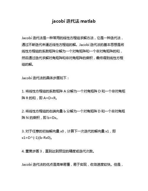
jacobi迭代法matlabJacobi迭代法是一种常用的线性方程组求解方法,它是一种迭代法,通过不断迭代来逼近线性方程组的解。
Jacobi迭代法的基本思想是将线性方程组的系数矩阵分解为一个对角矩阵和一个非对角矩阵的和,然后通过迭代求解对角矩阵和非对角矩阵的乘积,最终得到线性方程组的解。
Jacobi迭代法的具体步骤如下:1. 将线性方程组的系数矩阵A分解为一个对角矩阵D和一个非对角矩阵R的和,即A=D+R。
2. 将线性方程组的右端向量b分解为一个对角矩阵D和一个非对角矩阵N的乘积,即b=Dx。
3. 对于任意的初始解向量x0,计算下一次迭代的解向量x1,即x1=D^(-1)(b-Rx0)。
4. 重复步骤3,直到达到预定的精度或迭代次数。
Jacobi迭代法的优点是简单易懂,易于实现,收敛速度较快。
但是,它的缺点也很明显,即收敛速度较慢,需要进行大量的迭代才能达到较高的精度。
在Matlab中,可以使用以下代码实现Jacobi迭代法:function [x,k]=jacobi(A,b,x0,tol,maxit)% Jacobi迭代法求解线性方程组Ax=b% 输入:系数矩阵A,右端向量b,初始解向量x0,精度tol,最大迭代次数maxit% 输出:解向量x,迭代次数kn=length(b); % 系数矩阵A的阶数D=diag(diag(A)); % 对角矩阵DR=A-D; % 非对角矩阵Rx=x0; % 初始解向量for k=1:maxitx1=D\(b-R*x); % 计算下一次迭代的解向量if norm(x1-x)<tol % 判断是否达到精度要求break;endx=x1; % 更新解向量end输出结果可以使用以下代码实现:A=[4 -1 0; -1 4 -1; 0 -1 4]; % 系数矩阵b=[15; 10; 10]; % 右端向量x0=[0; 0; 0]; % 初始解向量tol=1e-6; % 精度要求maxit=1000; % 最大迭代次数[x,k]=jacobi(A,b,x0,tol,maxit); % Jacobi迭代法求解线性方程组fprintf('解向量x=[%f; %f; %f]\n',x(1),x(2),x(3)); % 输出解向量fprintf('迭代次数k=%d\n',k); % 输出迭代次数以上就是Jacobi迭代法的主要内容,通过Matlab实现Jacobi迭代法可以更好地理解其基本思想和具体步骤。
matlabjacobi迭代法
matlabjacobi迭代法Jacobi迭代法是一种求解线性方程组的迭代法,其基本思想是将原方程组的系数矩阵分解为对角部分和非对角部分,对于对角矩阵使用前、后代替法求解,对于非对角部分使用迭代更新法求解。
Jacobi迭代法的基本形式如下:$\begin{cases}a_{11}x_1+a_{12}x_2+...+a_{1n}x_n=b_1 \\a_{21}x_1+a_{22}x_2+...+a_{2n}x_n=b_2 \\... \\a_{n1}x_1+a_{n2}x_2+...+a_{nn}x_n=b_n \\\end{cases}$其中,$a_{ij}$表示系数矩阵的第$i$行第$j$列的元素,$b_i$表示方程组的第$i$个方程的解。
设向量$x^{(k)}=(x_1^{(k)},x_2^{(k)},...,x_n^{(k)})$表示Jacobi迭代法的第$k$次迭代结果,则迭代公式为:$x_i^{(k+1)}=\frac{1}{a_{ii}}(b_i-\sum_{j=1,j\ne i}^n a_{ij}x_j^{(k)}),i=1,2,...,n$迭代公式的意义是,将第$i$个变量的系数$a_{ii}$看成系数矩阵的一个主对角元,将剩下的系数$a_{ij}(i\ne j)$看成非对角元,同时将当前未知量向量$x^{(k)}$看成已知量,利用这些参数求解第$i$个方程中未知量$x_i$。
Jacobi迭代法的收敛条件为原矩阵的对角线元素不为零,且矩阵的任意一行中非对角线元素绝对值之和小于对角线元素绝对值。
在Matlab中,可通过编写函数的方式实现Jacobi迭代法。
函数jacobi实现了迭代公式,并以向量形式返回迭代结果,如下所示:```function xnew = jacobi(A, b, xold)% Jacobi迭代法求解线性方程组Ax=b% A为系数矩阵,b为常数向量,xold为迭代初值% 输出迭代后的解向量xnew% 初始化迭代初值n = length(b);xnew = zeros(n,1);% 迭代更新for i = 1:nxnew(i) = (b(i) - A(i,:)*xold + A(i,i)*xold(i)) / A(i,i);endend```在主程序中可按以下步骤使用函数jacobi求解线性方程组:1.构造系数矩阵A和常数向量b;2.设定迭代初值xold;3.利用jacobi函数求解迭代结果,并对迭代过程进行循环。
用共轭梯度法解方程,用Jacobi方法求矩阵的全部特征值和特征向量
end
A(1,1)=4;
A(n,n)=4;
A(n,n-1)=1;
X=zeros(n,1);
fori=1:n
X(i,1)=1;
end
%用共轭梯度法求解方程
fprintf('方程的精确解\n');
X
fprintf('用共轭法求解方程\n');
x=cg(A,b)
%用方法求解方程的特征值和特征向量
-0.1859 -0.0000 0.0000 0.0000 5.6180 -0.0000 -0.0000
-0.2236 0.0000 -0.0000 0.0000 0.0000 5.4142 0.0000
-0.2558 0.0000 -0.0000 0.0000 0.0000 0.0000 5.1756
0.1859 -0.0000 -0.0000 -0.0000 -0.0000 0.0000 -0.0000
0.1436 -0.0000 -0.0000 -0.0000 0.0000 -0.0000 0.0000
-0.0977 0.0000 0.0000 -0.0000 0.0000 -0.0000 0.0000
0.6634
1.1794
0.6188
1.3453
用方法Jacobi求解矩阵的全部特征值及特征向量
D =
Columns 1 through 7
4.0000 0 0 0 0 0 0
0.1382 5.9021 0.0000 0.0000 -0.0000 0.0000 0.0000
-0.2629 0.0000 5.6180 0.0000 0.0000 -0.0000 -0.0000
(k)Jacobi矩阵特征值反问题算法的稳定性分析
AbstractIfwedon,tknowtheJacobimatrix正m,butweknowalleigen—valuesofmatrixT1.1—1,alleigenvaluesofmatrixTk+l,n,andalleigen’valuesofmatrixT1m,couldweconstructthematrix乃,n.Le七S1==(芦1,p2,…,pk—1),S2=(弘七,p七+1,…,∥n一1),A=(A1,A2,…,An)a,retheeigenvaluesofmatrices乃,≈一1,Tk+l,nand丑,nrespectively.Theproblemisthatfromabove2n-1datatofindother2n-1data:a1,a2,…,dn,and卢1,岛,…,风一1Obviously,whenk=lork=nthisproblemhasbeensolvedandtherearemanyalgorithmstoconstruct乃,”【3】[6儿9】,anditsstabilityanalysiscanbefoundedinf21.Wrhile南=2,3…佗一1,anewalgorithmhasbeenputforwardtoconstruct乃,"【1】.Inthispaperwewillgivesomek=2.3…n一1.stabilityqualitiesofthenewalgorithmincaseInthispaperwewillanalyzetheperturbationqualityforanewalgorithmofthe(k1Jacobimatrixinverseeigenvalueproblem.Andfinallytaketheconclusionthatthealgorithmofthe(k)JacobiinverseproblemisLipschitzcontinuous.Keywords:Jacobimatrix,(k)inverseproblem,stabilaty,eigen-value.上海大学本论文经答辩委员会全体委员审查,确认符合上海大学硕士学位论文质量要求。
matlab中jacobi迭代法
一、简介Matlab中jacobi迭代法是一种用于求解线性方程组的迭代方法,适用于系数矩阵为对称、正定矩阵的情况。
该迭代方法通过将系数矩阵分解为对角矩阵、上三角矩阵和下三角矩阵的形式,然后通过迭代计算得到方程组的解。
在Matlab中,可以利用矩阵运算和迭代循环来实现jacobi迭代法。
二、 jacobi迭代法原理1. 基本思想jacobi迭代法的基本思想是将系数矩阵分解为对角矩阵D、上三角矩阵U和下三角矩阵L的形式,即A=D+L+U,其中D为系数矩阵A 的对角线元素组成的对角矩阵,L为系数矩阵A的下三角部分,U为系数矩阵A的上三角部分。
令x为方程组的解向量,b为方程组的右端向量,则方程组可表示为Ax=b。
根据方程组的性质,可将方程组表示为(D+L+U)x=b,然后利用迭代的方式逐步逼近方程组的解。
2. 迭代公式假设迭代到第k次,方程组可表示为(D+L+U)x=b,将其转化为迭代形式x(k+1)=(D+L)^(-1)(b-Ux(k)),利用迭代公式可以逐步计算出方程组的解。
3. 收敛条件对于jacobi迭代法,收敛条件为系数矩阵A为对角占优矩阵或正定矩阵。
如果满足这一条件,迭代计算会逐步收敛于方程组的解。
三、 Matlab中jacobi迭代法实现在Matlab中,可以利用矩阵运算和迭代循环来实现jacobi迭代法。
具体步骤如下:1. 对系数矩阵进行分解将系数矩阵A分解为对角矩阵D、上三角矩阵U和下三角矩阵L的形式。
2. 初始化迭代变量初始化迭代的初始值x0、迭代次数k、逐次逼近解向量x(k+1)。
3. 迭代计算利用迭代公式x(k+1)=(D+L)^(-1)(b-Ux(k))来逐步计算出方程组的解。
4. 判断收敛条件在迭代计算过程中,需要实时判断迭代计算是否满足收敛条件,如果满足则停止迭代计算,得到方程组的解。
四、实例分析假设有如下方程组:2x1 + x2 + 4x3 = 103x1 + 4x2 - x3 = 10x1 + 2x2 + 3x3 = 0可以利用jacobi迭代法来求解该方程组,在Matlab中可以通过编程实现迭代计算过程。
- 1、下载文档前请自行甄别文档内容的完整性,平台不提供额外的编辑、内容补充、找答案等附加服务。
- 2、"仅部分预览"的文档,不可在线预览部分如存在完整性等问题,可反馈申请退款(可完整预览的文档不适用该条件!)。
- 3、如文档侵犯您的权益,请联系客服反馈,我们会尽快为您处理(人工客服工作时间:9:00-18:30)。
2 An Analysis of the RTZ Algorithm
We now show that when applying the RTZ algorithm,
we can only obtain at best a linear convergence rate if the
matrix has complex eigenvalues.
through unitary similarity transformations
QAQ¯ T = D
where Q is unitary and D is diagonal. In this paper we
consider how to design a scalable Jacobi-like algorithm for efficient parallel computation of the eigenvalue decomposition of a real normal matrix over the real field. Real normal matrices are generalisations of real symmetric matrices. A real symmetric matrix is normal, but a real normal matrix is not necessarily symmetric. We shall focus our attention on the unsymmetric case although the method to be described applies to both cases.
In this paper we describe a method for designing efficient Jacobi-like algorithms for eigenvalue decomposition of a real normal matrix. The designed algorithms use only real arithmetic and orthogonal similarity transformations. The theoretical analysis and experimental results show that ultimate quadratic convergence can be achieved for general real normal matrices with distinct eigenvalues.
erate a Householder matrix which is then applied to update
the matrix A so that two off-diagonal elements a31 and a41
are annihilated. After that the second leading diagonal ele-
1 Introduction
A real matrix A is said to be normal if it satisfies the
equation
AAT = AT A
where AT is the transpose of matrix A. This kind of matrix
has the property that it can be reduced to a diagonal form
this method a 4 4 symmetric matrix can be reduced to a 2 2 block diagonal form using one orthogonal similar-
ity transformation. This method can also be extended to compute eigenvalues of a general normal matrix. However, the problems are that the original matrix has to be divided into a sum of a symmetric matrix and a skew-symmetric matrix, which is not an orthogonal operation, and that the algorithm cannot be used to solve the eigenvalue problem of near-normal matrices. Another parallel Jacobi-like algorithm, named the RTZ (which stands for Real Two-Zero) algorithm, was also proposed recently [5]. This method uses real arithmetic and orthogonal similarity transformations. It is claimed that quadratic convergence can be obtained when computing eigenvalues of a real near-normal matrix with real distinct eigenvalues. However, a serious problem with this method is that the process may not converge if the matrix has complex eigenvalues.
பைடு நூலகம்
tTghehetehwefirhrowstlieltehoaftdhAien2gfi2 rdtsoitafrgooorwnmailnae3Ale1m2,e3tnhmteaafit1rr1isxtin,ctoAhlau1t1misins,
chosen to-
A in 21 and
0@ 1A A1 =
a11 a31 a41
a13 a33 a43
a14 a34 a44
:
It is known that any real 3 3 matrix has at least one real
eigenvalue. An eigenvector associated with a real eigen-
value of the above matrix can be obtained and used to gen-
Jacobi-like Algorithms for Eigenvalue Decomposition of a Real Normal Matrix Using Real Arithmetic
B. B. Zhou and R. P. Brent Computer Sciences Laboratory The Australian National University Canberra, ACT 0200, Australia fbing,rpbg@.au
;
is used to show how the convergence rate may be affected
when applying the RTZ algorithm.
The basic idea for computing the eigenvalue decomposi-
tion of a 4 4 matrix using the RTZ algorithm is as follows:
Since the RTZ algorithm uses a similar idea to our method, an analysis of the RTZ algorithm is presented in Section 2. Our method is described in Section 3. In that section a theoretical analysis of convergence is also presented. Some experimental results are given in Section 4. Section 5 is the conclusion.
The Jacobi method, though originally designed for symmetric eigenvalue problems, can be extended to solve eigenvalue problems for unsymmetric normal matrices [3, 7]. However, one problem is that we have to use complex arithmetic even for real-valued normal matrices. Complex operations are expensive and should be avoided if possible. A quaternion-Jacobi method was recently introduced [4]. In
The standard sequential method for eigenvalue decomposition of this kind of matrix is the QR algorithm. When massively parallel computation is considered, however, the parallel version of the QR algorithm for solving unsymmetric eigenvalue problems may not be very efficient because the algorithm is sequential in nature and not scalable.