西电数据挖掘大作业k-means和k-medoids
聚类算法 KNN 、K-mean ,K-center FCM
聚类算法分类
划分方法(partitioning method)k-means 层次方法(hierarchical methods) 基于密度的方法(density-based methods) 基于网格的方法(grid-based methods) 基于模型的方法(model-based methods)
Eg:样本点A –>E1=10 样本点B –>E2=11 样本点C –>E3=12 原质点O–>E4=13, 那我们选举A作为类簇的新质点。与K-means算法一样, K-medoids也是采用欧几里得距离来衡量某个样本点 到底是属于哪个类簇。终止条件是,当所有的类簇的 质点都不在发生变化时,即认为聚类结束。
K-MEANS
算法流程:
首先从聚类对象中随机选出K个对象作为类簇 的质心(当然了,初始参数的K代表聚类结果 的类簇数),对剩余的每个对象,根据它们分 别到这个K个质心的距离,将它们指定到最相 似的簇(因为K-means是利用距离来量化相似 度的,所以我们这里可以理解为是“将它们指 定到离最近最近距离的质心所属类簇”)。然 后重新计算质心位置。以上过程不断反复,直 到准则函数收敛为止。
K-MEANS
算法流程:
通常采用平方误差准则,定义如下:
其中,E代表的意思是所有类簇中各对象到其所属类簇 质点平方误差和. K:聚类结果类簇个数 Ci:第i个类簇 P:类簇中聚类对象mi:第i个类簇的质心
K-MEANS
K-MEANS
优点与不足:
优点: 能处理大型数据集,结果簇相当紧凑,并且簇和 簇之间明显分离。 不足: 1)该算法必须事先给定类簇数和质点,簇数和 质点的初始值设定往往会对聚类的算法影响较 大。 2 ) 通常会在获得一个局部最优值时停止。
k-medoids 聚类公式字母公式
k-medoids 聚类算法是一种常用的基于距离的聚类方法,它主要用于将数据集中的数据点划分为若干个类别,使得同一类别内的数据点之间的相似度较高,不同类别之间的相似度较低。
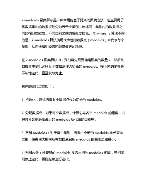
与k-means 算法不同的是,k-medoids 算法使用代表性的数据点(medoids)来代表每个类别,从而使得对噪声和异常值更加稳健。
在k-medoids 聚类算法中,我们首先需要确定聚类的数量k,然后从数据集中随机选择k个数据点作为初始的medoids。
接下来的步骤是不断地迭代,直至收敛为止。
具体的迭代过程如下:1. 初始化:随机选择k个数据点作为初始的medoids。
2. 分配数据点:对于每个数据点,计算它与各个medoids 的距离,并将其分配到距离最近的medoids 所代表的类别中。
3. 更新medoids:对于每个类别,选择一个新的medoids 来代表该类别,使得该类别内所有数据点到新medoids 的距离之和最小。
4. 判断收敛:检查新的medoids 是否与旧的medoids 相同,若相同则停止迭代,否则继续进行迭代。
在k-medoids 聚类算法中,距离的计算可以使用各种不同的距离度量方式,例如欧氏距离、曼哈顿距离等。
对于大规模的数据集,k-medoids 算法可能会比k-means 算法更具有优势,因为它在每次迭代时只需要计算medoids 之间的距离,而不需要计算所有数据点之间的距离,从而可以减少计算量。
k-medoids 聚类算法是一种有效且稳健的聚类方法,它在处理一些特定情况下可以取得比k-means 更好的聚类效果。
通过对数据进行有效的分组和分类,k-medoids 聚类算法在数据挖掘和模式识别领域具有广泛的应用前景。
K-medoids clustering algorithm is a widely used distance-based clustering method for partitioning the data points in a dataset into several categories, in which the similarity of data points within the same category is relatively high, while the similarity between different categories is relatively low. Unlike the k-means algorithm, the k-medoids algorithm uses representative data points (medoids) to represent each category, making it more robust to noise and outliers.In the k-medoids clustering algorithm, the first step is to determine the number of clusters, denoted as k, and then randomly select k data points from the dataset as the initial medoids. The following steps involve iterative processes until the algorithm converges.The specific iterative process is as follows:1. Initialization: randomly select k data points as the initial medoids.2. Data point assignment: for each data point, calculate its distance to each medoid and assign it to the category represented by the nearest medoid.3. Update medoids: for each category, select a new medoid to represent the category, so that the sum of the distances from all data points in the category to the new medoid is minimized.4. Convergence check: check whether the new medoids are the same as the old medoids. If they are the same, stop the iteration; otherwise, continue the iteration.In the k-medoids clustering algorithm, various distance metrics can be used for distance calculation, such as Euclidean distance, Manhattan distance, etc. For large-scale datasets, the k-medoids algorithm may have advantages over the k-means algorithm because it only needs to calculate the distance betweenmedoids at each iteration, rather than calculating the distance between all data points, which can reduce theputational workload.In conclusion, the k-medoids clustering algorithm is an effective and robust clustering method that can achieve better clustering results than the k-means algorithm in certain situations. By effectively grouping and classifying data, the k-medoids clustering algorithm has wide application prospects in the fields of data mining and pattern recognition.Moreover, the k-medoids algorithm can be further extended and applied in various domains, such as customer segmentation in marketing, anomaly detection in cybersecurity, and image segmentation inputer vision. In marketing, k-medoids clustering can be used to identify customer segments based on their purchasing behavior, allowingpanies to tailor their marketing strategies to different customer groups. In cybersecurity, k-medoids can help detect anomalies by identifying patterns that deviate from the norm in network traffic or user behavior. Inputer vision, k-medoids can be used for image segmentation to partition an image into different regions based on similarity, which is useful for object recognition and scene understanding.Furthermore, the k-medoids algorithm can also bebined with other machine learning techniques, such as dimensionality reduction, feature selection, and ensemble learning, to improve its performance and scalability. For example, using dimensionality reduction techniques like principalponent analysis (PCA) can help reduce theputational burden of calculating distances in high-dimensional data, while ensemble learning methods like boosting or bagging can enhance the robustness and accuracy of k-medoids clustering.In addition, research and development efforts can focus on optimizing the k-medoids algorithm for specific applications and datasets, such as developing parallel and distributed versions of the algorithm to handle big data, exploring adaptive and dynamic approaches to adjust the number of clusters based on the data characteristics, and integrating domain-specific knowledge or constraints into the clustering process to improve the interpretability and usefulness of the results.Overall, the k-medoids clustering algorithm is a powerful tool for data analysis and pattern recognition, with a wide range of applications and potential for further advancements andinnovations. Its ability to handle noise and outliers, its flexibility in distance metrics, and its scalability to large-scale datasets make it a valuable technique for addressing real-world challenges in various domains. As the field of data science and machine learning continues to evolve, the k-medoids algorithm will likely remain an important method for uncovering meaningful insights fromplex data.。
k-medoids算法
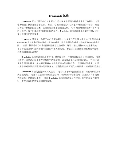
k-medoids算法K-medoids算法(基于中心对象算法)是一种属于聚类分析的非常流行的算法,它不像K-means算法那样基于质心。
相反,它使用最近的中心对象作为聚类的一部分。
聚类分析是一种数据挖掘技术,它搜索数据集中隐藏的关联。
它将测量对象组合到许多不同的分组中,每个组都具有相同或相似的属性。
K-medoids算法通过使用相似度度量,将对象分组到不同的类别中。
K-medoids算法是一种基于中心点聚类算法,它使用迭代计算来重复地优化聚类结果。
K-medoids算法从数据集中选择一组中心对象,然后将剩余的对象与最接近的中心对象分配。
然后,算法将中心对象更新以更接近这些对象,这可以通过调整中心对象来完成。
中心对象的改变引起的影响可能会影响聚类的结果。
K-medoids算法继续重复这个过程,直到找到聚类的最优解。
K-medoids算法在许多应用中使用,包括簇分析、序列模式探索和可视化聚类。
在簇分析中,该算法可以用来发现数据中的簇结构,以改善商业活动和市场分析。
它也可以用于发现序列模式,例如揭示隐藏在大型数据集中的共同行为。
在可视化聚类中,它可以用于将对象聚类到空间中的不同区域,以便使用空间可视化来观察簇的相似性和差异性。
K-medoids算法的优势在于其灵活性。
它可以用于不同类型的数据,而且可以应用于大型数据集。
它还可以适应非凸形数据结构,可以应用于低维空间,并且在具有多类噪声的情况下也能良好工作。
尽管K-medoids算法的算法复杂性较大,但它的稳定性非常好,对发现有用的数据结构非常有效。
k-medoids聚类算法
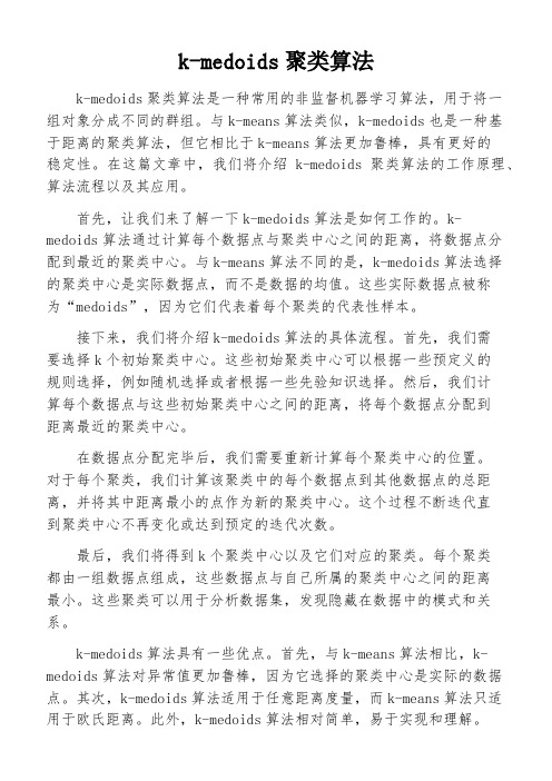
k-medoids聚类算法k-medoids聚类算法是一种常用的非监督机器学习算法,用于将一组对象分成不同的群组。
与k-means算法类似,k-medoids也是一种基于距离的聚类算法,但它相比于k-means算法更加鲁棒,具有更好的稳定性。
在这篇文章中,我们将介绍k-medoids聚类算法的工作原理、算法流程以及其应用。
首先,让我们来了解一下k-medoids算法是如何工作的。
k-medoids算法通过计算每个数据点与聚类中心之间的距离,将数据点分配到最近的聚类中心。
与k-means算法不同的是,k-medoids算法选择的聚类中心是实际数据点,而不是数据的均值。
这些实际数据点被称为“medoids”,因为它们代表着每个聚类的代表性样本。
接下来,我们将介绍k-medoids算法的具体流程。
首先,我们需要选择k个初始聚类中心。
这些初始聚类中心可以根据一些预定义的规则选择,例如随机选择或者根据一些先验知识选择。
然后,我们计算每个数据点与这些初始聚类中心之间的距离,将每个数据点分配到距离最近的聚类中心。
在数据点分配完毕后,我们需要重新计算每个聚类中心的位置。
对于每个聚类,我们计算该聚类中的每个数据点到其他数据点的总距离,并将其中距离最小的点作为新的聚类中心。
这个过程不断迭代直到聚类中心不再变化或达到预定的迭代次数。
最后,我们将得到k个聚类中心以及它们对应的聚类。
每个聚类都由一组数据点组成,这些数据点与自己所属的聚类中心之间的距离最小。
这些聚类可以用于分析数据集,发现隐藏在数据中的模式和关系。
k-medoids算法具有一些优点。
首先,与k-means算法相比,k-medoids算法对异常值更加鲁棒,因为它选择的聚类中心是实际的数据点。
其次,k-medoids算法适用于任意距离度量,而k-means算法只适用于欧氏距离。
此外,k-medoids算法相对简单,易于实现和理解。
k-medoids算法在许多领域都有广泛的应用。
聚类算法比较
聚类算法:1. 划分法:K-MEANS算法、K-M EDOIDS算法、CLARANS算法;1)K-means 算法:基本思想是初始随机给定K个簇中心,按照最邻近原则把待分类样本点分到各个簇。
然后按平均法重新计算各个簇的质心,从而确定新的簇心。
一直迭代,直到簇心的移动距离小于某个给定的值。
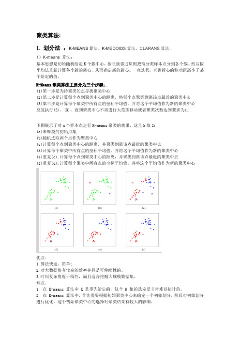
K-Means聚类算法主要分为三个步骤:(1)第一步是为待聚类的点寻找聚类中心(2)第二步是计算每个点到聚类中心的距离,将每个点聚类到离该点最近的聚类中去(3)第三步是计算每个聚类中所有点的坐标平均值,并将这个平均值作为新的聚类中心反复执行(2)、(3),直到聚类中心不再进行大范围移动或者聚类次数达到要求为止下图展示了对n个样本点进行K-means聚类的效果,这里k取2:(a)未聚类的初始点集(b)随机选取两个点作为聚类中心(c)计算每个点到聚类中心的距离,并聚类到离该点最近的聚类中去(d)计算每个聚类中所有点的坐标平均值,并将这个平均值作为新的聚类中心(e)重复(c),计算每个点到聚类中心的距离,并聚类到离该点最近的聚类中去(f)重复(d),计算每个聚类中所有点的坐标平均值,并将这个平均值作为新的聚类中心优点:1.算法快速、简单;2.对大数据集有较高的效率并且是可伸缩性的;3.时间复杂度近于线性,而且适合挖掘大规模数据集。
缺点:1. 在 K-means 算法中 K 是事先给定的,这个 K 值的选定是非常难以估计的。
2. 在 K-means 算法中,首先需要根据初始聚类中心来确定一个初始划分,然后对初始划分进行优化。
这个初始聚类中心的选择对聚类结果有较大的影响。
3. 从 K-means 算法框架可以看出,该算法需要不断地进行样本分类调整,不断地计算调整后的新的聚类中心,因此当数据量非常大时,算法的时间开销是非常大的。
4. 产生类的大小相差不会很大,对于脏数据很敏感。
2)K-M EDOIDS(k-medoids)算法与k-means很像,不一样的地方在于中心点的选取,在K-means中,我们将中心点取为当前cluster中所有数据点的平均值,在 K-medoids算法中,我们将从当前cluster 中选取这样一个点——它到其他所有(当前cluster中的)点的距离之和最小——作为中心点。
聚类分析—K-means and K-medoids聚类34页PPT

5、虽然权力是一头固执的熊,可是金 子可以 拉着它 的鼻子 走。— —莎士 比
ห้องสมุดไป่ตู้
6、最大的骄傲于最大的自卑都表示心灵的最软弱无力。——斯宾诺莎 7、自知之明是最难得的知识。——西班牙 8、勇气通往天堂,怯懦通往地狱。——塞内加 9、有时候读书是一种巧妙地避开思考的方法。——赫尔普斯 10、阅读一切好书如同和过去最杰出的人谈话。——笛卡儿
聚类分析—K-means and K-medoids聚 类
1、合法而稳定的权力在使用得当时很 少遇到 抵抗。 ——塞 ·约翰 逊 2、权力会使人渐渐失去温厚善良的美 德。— —伯克
3、最大限度地行使权力总是令人反感 ;权力 不易确 定之处 始终存 在着危 险。— —塞·约翰逊 4、权力会奴化一切。——塔西佗
k-medoids聚类算法
k-medoids聚类算法**标题:深入解析K-Medoids聚类算法****引言:**K-Medoids聚类算法是一种有效的数据聚类方法,广泛应用于数据挖掘、模式识别和机器学习领域。
相比于K-Means算法,K-Medoids在处理离群点时更为鲁棒,因为它选择代表性的样本作为簇的中心,而不是简单地计算样本的均值。
本文将深入探讨K-Medoids聚类算法的原理、步骤以及应用领域,以帮助读者更好地理解和应用这一强大的聚类算法。
**1. K-Medoids聚类算法简介:**K-Medoids聚类算法是一种基于中心点的聚类方法,旨在将数据集分为预定数量的簇,使得每个簇的内部数据点之间的相似度较高,而不同簇之间的相似度较低。
与K-Means算法不同,K-Medoids使用实际数据点作为簇的中心,而非简单地计算数据点的均值。
**2. K-Medoids算法的工作原理:**K-Medoids算法的核心思想是选择每个簇的代表性样本,即簇的中心点,以最小化簇内部数据点与中心点之间的距离。
算法的工作步骤如下:- **初始化:** 随机选择k个数据点作为初始的簇中心。
- **簇分配:** 将每个数据点分配到最近的簇中心,形成k个簇。
- **中心更新:** 对于每个簇,选择一个新的中心,使得该簇内所有数据点到新中心的总距离最小。
- **收敛判定:** 重复簇分配和中心更新步骤,直到簇中心不再改变或改变微小,达到收敛。
**3. K-Medoids与K-Means的比较:**- **鲁棒性:** K-Medoids相比K-Means对离群点更为鲁棒,因为中心点是实际数据点,不受异常值的影响。
- **复杂度:** 由于K-Medoids需要计算中心点到所有其他数据点的距离,算法的复杂度相对较高,但在小规模数据集上表现良好。
- **收敛性:** K-Medoids的收敛性较差,且初始中心点的选择对结果影响较大。
**4. K-Medoids算法的改进和优化:**- **PAM算法:** Partitioning Around Medoids(PAM)是K-Medoids的经典算法,通过交换中心点与非中心点来优化簇的内部距离。
k-medoids算法
k-medoids算法k-medoids算法是一种用于聚类分析的算法。
它与k-means算法相似,但有一些不同之处。
在k-means算法中,每个聚类的中心点是所属聚类中的所有样本的均值。
而在k-medoids算法中,每个聚类的中心点是聚类中的一个实际样本点,也称为medoid。
1. 随机选择k个样本作为初始medoids。
2. 对于每个样本,计算其与每个medoid的距离,并将其分配到距离最近的medoid所属的聚类中。
3. 对于每个聚类,计算其中所有样本与其medoid的总距离。
选取总距离最小的样本作为新的medoid。
4. 重复步骤2和步骤3,直到medoid不再改变或达到最大迭代次数。
5.得到最终的聚类结果。
1. 对于离群点更加鲁棒:由于medoid是聚类中的实际样本点,而不是均值点,因此k-medoids算法对于存在离群点的数据集更加鲁棒。
2. 可以应用于非欧几里德距离度量:k-means算法基于欧几里德距离,而k-medoids算法可以灵活地使用非欧几里德距离度量,例如曼哈顿距离或闵可夫斯基距离。
3. 可解释性更强:由于medoid是具体的样本点,而不是均值点,这意味着聚类结果更容易理解和解释。
k-medoids算法的应用广泛。
例如,在医学领域,它可以用于将患者分为不同的疾病类别,从而有助于疾病的诊断和治疗。
在市场营销中,它可以用于消费者分组,以便制定个性化的推广策略。
在图像处理领域,它可以用于图像分割,将相似的像素聚类在一起。
然而,k-medoids算法也存在一些局限性。
首先,由于需要计算样本之间的距离,如果数据集非常大,计算成本会很高。
其次,k-medoids算法对于数据集中选择medoids的敏感度较高,不同的初始medoids可能会导致不同的聚类结果。
此外,k-medoids算法无法直接处理高维数据,需要使用降维方法来减少维度。
为了克服这些局限性,研究人员提出了一些改进的k-medoids算法,如PAM算法和CLARA算法。
常规聚类算法
常规聚类算法常规聚类算法是一种重要的数据分析方法,可以帮助我们对大规模数据进行有效的分类和归纳。
通过对数据进行聚类,我们可以发现数据中的隐藏模式、规律和关系,从而为后续的数据挖掘、预测和决策提供有力支持。
常规聚类算法主要分为基于划分的聚类算法、基于层次的聚类算法和基于密度的聚类算法。
每种算法都有其独特的特点和适用场景,下面就分别进行介绍。
基于划分的聚类算法主要包括K-means算法和K-medoids算法。
K-means算法是一种常用且广泛应用的聚类算法,它将数据分成K个簇,每个簇的中心点代表了该簇的平均值。
该算法通过迭代的方式,将数据点不断归类到离其最近的簇中,直到达到稳定状态。
K-medoids算法是一种改进的K-means算法,它将簇的中心点定义为簇中所有数据点中与其他点的平均距离最小的点,从而可以更准确地划分簇。
基于层次的聚类算法主要包括凝聚层次聚类算法和分裂层次聚类算法。
凝聚层次聚类算法从每个数据点作为一个簇开始,然后通过计算两个最相似簇之间的距离来合并簇,直到形成一个大的簇。
分裂层次聚类算法则相反,从一个大的簇开始,然后通过计算簇中数据点之间的距离来分裂簇,直到形成多个小的簇。
这种算法的优点是可以在不同的层次上进行聚类,从而可以灵活地控制聚类的粒度。
基于密度的聚类算法主要包括DBSCAN算法和OPTICS算法。
DBSCAN算法是一种基于密度的聚类算法,它通过确定数据点的密度来划分簇,具有自动确定簇数和可处理噪声的优点。
OPTICS算法是DBSCAN算法的扩展,它通过将数据点的密度和可达距离进行排序,形成一个密度可达图,并根据该图来划分簇。
这种算法可以更好地处理数据中的离群点和噪声。
在使用常规聚类算法时,我们需要注意数据的选择和预处理。
合适的数据选择和预处理可以提高聚类算法的效果和准确性。
同时,我们还需要关注聚类结果的解释和评估。
解释聚类结果可以帮助我们理解数据中的模式和关系,评估聚类结果可以帮助我们判断算法的优劣和稳定性。
k-medoids聚类算法
k-medoids聚类算法
k-medoids聚类算法又叫做PAM算法,是一种基于中心点的分组聚类算法,和k-means算法相似,其目的也是将样本划分为k个簇,每个簇都包含距离簇中心最近的样本点。
与k-means不同的是,k-medoids使用的是样本点而非均值点来作为簇的中心点,因此不受离群点的影响,在一定程度上提高了聚类的准确性。
k-medoids算法的步骤如下:
1. 随机选择k个样本作为初始中心点。
2. 将每个样本点分配到与其最近的中心点所在的簇中。
3. 计算每个簇中所有样本之间的距离和作为该簇的代价函数。
4. 针对每个簇中的每个样本,计算将该样本作为中心点后,该簇的代价函数。
5. 如果将当前簇的某个样本作为中心点可以降低该簇的代价函数,则将该样本作为新的中心点。
6. 重复执行步骤2至5,直到簇的中心点不再改变。
最终,k-medoids算法会得到k个簇,每个簇包含距离中心点最近的一些样本点。
通过对数据的分析,可以发现不同的簇之间具有明显的差异性,对于簇内相似性高、簇间相似性低的数据集,k-medoids 算法在实际应用中有着广泛的应用。
- 1、下载文档前请自行甄别文档内容的完整性,平台不提供额外的编辑、内容补充、找答案等附加服务。
- 2、"仅部分预览"的文档,不可在线预览部分如存在完整性等问题,可反馈申请退款(可完整预览的文档不适用该条件!)。
- 3、如文档侵犯您的权益,请联系客服反馈,我们会尽快为您处理(人工客服工作时间:9:00-18:30)。
题 目: 数据挖掘学 院: 电子工程学院专 业: 智能科学和技术学生姓名: **学 号: 02115***k -means 实验报告一、 waveform 数据1、 算法描述1. 从数据集{X n }n−1N 中任意选取k 个赋给初始的聚类中心c 1, c 2, …,c k;2.对数据集中的每个样本点x i,计算其和各个聚类中心c j的欧氏距离并获取其类别标号:label(i)=arg min ||x i−c j||2,i=1,…,N,j=1,…,k3.按下式重新计算k个聚类中心;c j=∑x js:label(s)=jj,j=1,2,…k重复步骤2和步骤3,直到达到最大迭代次数为止2、实验结果二、图像处理1、算法描述同上;2、实验结果代码:k_means:%%%%%%%%%K_means%%%%%%%%%%%%%%%%%函数说明%%%%%%%%%输入:% sample——样本集;% k ——聚类数目;%输出:% y ——类标(从0开始)% cnew ——聚类中心% n ——迭代次数function [y cnew n]=k_means(sample,k)[N V]=size(sample); %N为样本的个数 K为样本的维数y=zeros(N,1); %记录样本类标dist=zeros(1,k);rand_num=randperm(N);cnew=(sample(rand_num(1,1:k),:));%随机初始化聚类中心cold=zeros(k,V);n=0;while(cold~=cnew)cold=cnew;n=n+1; %记录迭代次数%对样本进行重新分类for i=1:Nfor j=1:kif(V==1)dist(1,j)=abs(sample(i,:)-cold(j,:));elsedist(1,j)=norm(sample(i,:)-cold(j,:));endendfor s=1:kif(dist(1,s)==min(dist))y(i,1)=s-1;endendend%更新聚类中心cnew=zeros(k,V);flag=zeros(k,1);for i=1:Nfor j=1:kif (y(I,1)==j-1)flag(j,1)=flag(j,1)+1;cnew(j,☺=cnew(j,☺+sample(I,☺;endendendfor j=1:kcnew(j,☺=cnew(j,☺/flag(j,1);endendk_means_waveform:clear;clc;%%%%%%%%%数据读入%%%%%%%data=load('G:\西电\2014大三下\大作业\Data Mining\k_means\waveform.data');[N K]=size(data); %数据集的数目data0=zeros(1,K);data1=zeros(1,K);data2=zeros(1,K);for i=1:Nif(data(i,K)==0)data0=cat(1,data(i,:),data0);elseif(data(i,K)==1)data1=cat(1,data(i,:),data1);elsedata2=cat(1,data(i,:),data2);endendsample=cat(1,data0(1:100,:),data1(1:100,:),data2(1:100,:));label=sample(:,K); %样本的正确类标sample=sample(:,1:K-1); %样本集k=3; %聚类中心的数目%%%%%%%%%K_means%%%%%%%%[y cnew n]=k_means(sample,k);%%%%%%%%%%正确率统计%%%%%%%sum=zeros(1,6);[N V]=size(sample);for i=1:Nif(y(i,1)==label(i,1))sum(1,1)=sum(1,1)+1;endendfor i=1:Nif((y(i,1)+label(i,1))==2)sum(1,2)=sum(1,2)+1;endendfor i=1:Nif(((y(i,1)==0)&&(label(i,1)==0))||((y(i,1)==1)&&label(i,1)==2)||((y( i,1)==2)&&label(i,1)==1))sum(1,3)=sum(1,3)+1;endendfor i=1:Nif(((y(i,1)==0)&&(label(i,1)==1))||((y(i,1)==1)&&label(i,1)==0)||((y( i,1)==2)&&label(i,1)==2))sum(1,4)=sum(1,4)+1;endendfor i=1:Nif(((y(i,1)==0)&&(label(i,1)==1))||((y(i,1)==1)&&label(i,1)==2)||((y( i,1)==2)&&label(i,1)==0))sum(1,5)=sum(1,5)+1;endendfor i=1:Nif(((y(i,1)==0)&&(label(i,1)==2))||((y(i,1)==1)&&label(i,1)==0)||((y( i,1)==2)&&label(i,1)==1))sum(1,6)=sum(1,6)+1;endendsum=sum/N;creatrate=max(sum);disp('循环次数:');disp(n);disp('聚类中心为:');disp(cnew);disp('正确率为:');disp(creatrate);k_means_picture:clear;clc;%%%%%%%%%数据读入%%%%%%%I1=imread('G:\西电\2014大三下\大作业\Data Mining\ k_means\lena.jpg');I2=rgb2gray(I1);%转化为灰度图像I=im2double(I2);[num v]=size(I);sample=reshape(I,v*num,1);%样本集k=2; %聚类中心的数目%%%%%%%%%K_means%%%%%%%%[y cnew n]=k_means(sample,k);%%%%%%%%v%%%%%%%%I3=sample;if(cnew(1,1)>=cnew(2,1))F0=255;F1=0;elseF0=0;F1=255;endfor i=1:num*vif(y(i,1)==0)I3(i,1)=F0;elseI3(i,1)=F1;endendI3=reshape(I3,num,v);figure(1)subplot(1,3,1);imshow(I1);title('原图像');subplot(1,3,2);imshow(I2);title('灰度图像');subplot(1,3,3);imshow(I3);title('二值化图像');k_medoids实验报告一、 waveform数据1、算法描述(1)随机选择k个对象作为初始的代表对象;(2) repeat(3) 指派每个剩余的对象给离它最近的代表对象所代表的簇;(4) 随意地选择一个非代表对象Orandom;(5) 计算用Orandom代替Oj的总代价S;(6) 如果S<0,则用Orandom替换Oj,形成新的k个代表对象的集合;(7) until 不发生变化2、实验结果二、图像处理1、算法描述同上;2、实验结果代码:k_medoids:%%%%%%%%k_medoids%%%%%%%%%%%%%%%%%º函数说明%%%%%%%%%%输入:% sample——数据集% k——聚类数目;%输出:% y——类标;% med ——聚类中心点function [y med]=k_medoids(sample,k)[N V]=size(sample); %N为样本数目 V为样本为数%聚类中心的随机初始化rbowl=randperm(N);med=sample(rbowl(1,1:k),:);temp=zeros(N,2);dist=zeros(1,k);index=rbowl(1,k);Eold=0;Enew=1000;while(abs(Enew-Eold)>0.001)%将所有样本分配到最近的代表点for i=1:Nfor j=1:kdist(1,j)=norm(sample(i,:)-med(j,:));endtemp(i,1)=min(dist);for s=1:kif(dist(1,s)==temp(i,1))temp(i,2)=s;endendendy=temp(:,2);Eold=sum(temp(:,1));%随机的选择一个非代表点,生成新的代表点集合index=index+1;med_temp=med;E=zeros(1,k);for j=1:kmed_temp(j,:)=sample(index,:);%将所有样本分配到最近的代表点for i=1:Nfor t=1:kdist(1,t)=norm(sample(i,:)-med_temp(t,:));endtemp(i,1)=min(dist);for s=1:kif(dist(1,s)==temp(i,1))temp(i,2)=s;endendendE(1,j)=sum(temp(:,1));endEnew=min(E);for t=1:kif(E(1,t)==Enew)obest=t;endendif(Enew<Eold)med(obest,:)=sample(index,:);elseEnew=Eold;endendk_medoids_waveform:clear;clc;%%%%%%%%%Êý¾Ý¶ÁÈë%%%%%%%data=load(' G:\西电\2014大三下\大作业\Data Mining\k_medoids\waveform-+noise.data');[N K]=size(data); %数据集的数目data0=zeros(1,K);data1=zeros(1,K);data2=zeros(1,K);for i=1:Nif(data(i,K)==0)data0=cat(1,data(i,:),data0);elseif(data(i,K)==1)data1=cat(1,data(i,:),data1);elsedata2=cat(1,data(i,:),data2);endendsample=cat(1,data0(1:100,:),data1(1:100,:),data2(1:100,:)); label=sample(:,K); %Ñù±¾µÄÕýÈ·Àà±êsample=sample(:,1:K-1); %Ñù±¾¼¯k=3; %聚类中心的数目%%%%%%%%%%k_medoids%%%%%%%[y med]=k_medoids(sample,k);%%%%%%%%%%正确率统计Æ%%%%%%%sum=zeros(1,6);[N V]=size(sample);for i=1:Ny(i,1)=y(i,1)-1;endfor i=1:Nif(y(i,1)==label(i,1))sum(1,1)=sum(1,1)+1;endendfor i=1:Nif((y(i,1)+label(i,1))==2)sum(1,2)=sum(1,2)+1;endendfor i=1:Nif(((y(i,1)==0)&&(label(i,1)==0))||((y(i,1)==1)&&label(i,1)==2)||((y( i,1)==2)&&label(i,1)==1))sum(1,3)=sum(1,3)+1;endendfor i=1:Nif(((y(i,1)==0)&&(label(i,1)==1))||((y(i,1)==1)&&label(i,1)==0)||((y( i,1)==2)&&label(i,1)==2))sum(1,4)=sum(1,4)+1;endendfor i=1:Nif(((y(i,1)==0)&&(label(i,1)==1))||((y(i,1)==1)&&label(i,1)==2)||((y( i,1)==2)&&label(i,1)==0))sum(1,5)=sum(1,5)+1;endendfor i=1:Nif(((y(i,1)==0)&&(label(i,1)==2))||((y(i,1)==1)&&label(i,1)==0)||((y( i,1)==2)&&label(i,1)==1))sum(1,6)=sum(1,6)+1;endendsum=sum/N;creatrate=max(sum);disp('¾ÛÀàÖÐÐÄΪ£º');disp(med);disp('ÕýÈ·ÂÊΪ£º');disp(creatrate);k_medoids_picture:clear;clc;%%%%%%%%%Êý¾Ý¶ÁÈë%%%%%%%I0=imread(' G:\西电\2014大三下\大作业\Data Mining\ k_medoids\lena.jpg'); D=0.001;I1=imnoise(I0,'gaussian',0,D);%加噪声I2=rgb2gray(I1);%转化为灰度图像I=im2double(I2);[num v]=size(I);sample=reshape(I,v*num,1);%Ñù±¾¼¯k=2; %¾ÛÀàÖÐÐĵÄÊýÄ¿%%%%%%%%%K_means%%%%%%%%[y med]=k_medoids(sample,k); %%%%%%%%图像显示¾%%%%%%%%I3=sample;if(med(1,1)>=med(2,1))F0=255;F1=0;elseF0=0;F1=255;endfor i=1:num*vif(y(i,1)==1)I3(i,1)=F0;elseI3(i,1)=F1;endendI3=reshape(I3,num,v);figure(1)subplot(1,4,1);imshow(I0);title('原图像');subplot(1,4,2);imshow(I1);title('加噪声后的图像');subplot(1,4,3);imshow(I2);title('灰度图像');subplot(1,4,4);imshow(I3);title('二值化图像');。