投资学第10版习题答案09
投资学第9章习题及答案

本章习题1.简述利率敏感性的六个特征。
2.简述久期的法则。
3.凸性和价格波动之间有着怎样的关系?4.简述可赎回债券与不可赎回债券的凸性之间的区别。
5.简述负债管理策略中免疫策略的局限性。
6.简述积极的债券投资组合管理中互换策略的主要类型。
7.一种收益率为10%的9年期债券,久期为7.194年。
如果市场收益率改变50个基点,则债券价格变化的百分比是多少?8.某种半年付息的债券,其利率为8%,收益率为8%,期限为15年,麦考利久期为10年。
(1)利用上述信息,计算修正久期。
(2)解释为什么修正久期是计算债券利率敏感性的较好方法。
(3)确定修正久期变动的方向,如果:a.息票率为4%,而不是8%b.到期期限为7年而不是15年。
(4)说明在给定利率变化的情况下,修正久期与凸性是怎样用来估计债券价格变动的?第九章本章习题答案1. 在市场利率中,债券价格的敏感性变化对投资者而言显然十分重要。
为了了解利率风险的决定因素,可以参见图9-1。
该图表示四种债券价格相对于到期收益变化的变化百分比,它们有不同的息票率、初始到期收益率以及到期时间。
这四种债券的情况表明,当收益增加时,债券价格下降;价格曲线是凸的,这意味着收益下降对价格的影响远远大于等规模的收益增加。
通过观察,可以得出以下两个特征:(1)债券价格与收益呈反比,即:当收益升高时,债券价格下降;当收益上升时,债券价格上升。
(2)债券的到期收益升高会导致其价格变化幅度小于等规模的收益下降。
比较债券A和B的利率敏感性,除到期时间外,其他情况均基本相同。
图9-1表明债券B比债券A期限更长,对利率更敏感。
这体现出其另一特征:(3)长期债券价格对利率变化的敏感性比短期债券更高。
这不足为奇,例如,如果利率上涨,则当前贴现率较高,债券的价值下降。
由于利率适用于更多种类的远期现金流,则较高的贴现率的影响会更大。
值得注意的是,当债券B的期限是债券A的期限的6倍的时候,它的利率敏感性低于6倍。
投资学(博迪)第10版课后习题答...
投资学(博迪)第10版课后习题答...CHAPTER 10: ARBITRAGE PRICING THEORY ANDMULTIFACTOR MODELS OF RISK AND RETURN PROBLEM SETS1. The revised estimate of the expected rate of return on the stock would be the oldestimate plus the sum of the products of the unexpected change in each factor times the respective sensitivity coefficient: Revised estimate = 12% + [(1 × 2%) + (0.5 × 3%)] = 15.5%Note that the IP estimate is computed as: 1 × (5% - 3%), and the IR estimate iscomputed as: 0.5 × (8% - 5%).2. The APT factors must correlate with major sources of uncertainty, i.e., sources ofuncertainty that are of concern to many investors. Researchers should investigatefactors that correlate with uncertainty in consumption and investment opportunities.GDP, the inflation rate, and interest rates are among the factors that can be expected to determine risk premiums. In particular, industrial production (IP) is a goodindicator of changes in the business cycle. Thus, IP is a candidate for a factor that is highly correlated with uncertainties that have to do with investment andconsumption opportunities in the economy.3. Any pattern of returns can be explained if we are free to choose an indefinitelylarge number of explanatory factors. If a theory of asset pricing is to have value, itmust explain returns using a reasonably limited number of explanatory variables(i.e., systematic factors such as unemployment levels, GDP, and oil prices).4. Equation 10.11 applies here:E(r p) = r f + βP1 [E(r1 ) ?r f ] + βP2 [E(r2 ) – r f]We need to find the risk premium (RP) for each of the two factors:RP1 = [E(r1 ) ?r f] and RP2 = [E(r2 ) ?r f]In order to do so, we solve the following system of two equations with two unknowns: .31 = .06 + (1.5 ×RP1 ) + (2.0 ×RP2 ).27 = .06 + (2.2 ×RP1 ) + [(–0.2) ×RP2 ]The solution to this set of equations isRP1 = 10% and RP2 = 5%Thus, the expected return-beta relationship isE(r P) = 6% + (βP1× 10%) + (βP2× 5%)5. The expected return for portfolio F equals the risk-free rate since its beta equals 0.For portfolio A, the ratio of risk premium to beta is (12 ?6)/1.2 = 5For portfolio E, the ratio is lower at (8 – 6)/0.6 = 3.33This implies that an arbitrage opportunity exists. For instance, you can create aportfolio G with beta equal to 0.6 (the same as E’s) by combining portfolio A and portfolio F in equal weights. The expected return and beta for portfolio G are then: E(r G) = (0.5 × 12%) + (0.5 × 6%) = 9%βG = (0.5 × 1.2) + (0.5 × 0%) = 0.6Comparing portfolio G to portfolio E, G has the same betaand higher return.Therefore, an arbitrage opportunity exists by buying portfolio G and selling anequal amount of portfolio E. The profit for this arbitrage will ber G –r E =[9% + (0.6 ×F)] ?[8% + (0.6 ×F)] = 1%That is, 1% of the funds (long or short) in each portfolio.6. Substituting the portfolio returns and betas in the expected return-beta relationship,we obtain two equations with two unknowns, the risk-free rate (r f) and the factor risk premium (RP):12% = r f + (1.2 ×RP)9% = r f + (0.8 ×RP)Solving these equations, we obtainr f = 3% and RP = 7.5%7. a. Shorting an equally weighted portfolio of the ten negative-alpha stocks andinvesting the proceeds in an equally-weighted portfolio of the 10 positive-alpha stocks eliminates the market exposure and creates a zero-investmentportfolio. Denoting the systematic market factor as R M, the expected dollarreturn is (noting that the expectation of nonsystematic risk, e, is zero):$1,000,000 × [0.02 + (1.0 ×R M)] ? $1,000,000 × [(–0.02) + (1.0 ×R M)]= $1,000,000 × 0.04 = $40,000The sensitivity of the payoff of this portfolio to the market factor is zerobecause the exposures of the positive alpha and negative alpha stocks cancelout. (Notice that the terms involving R M sum to zero.) Thus, the systematiccomponent of total risk is also zero. The variance of the analyst’s profit is notzero, however, since this portfolio is not well diversified.For n = 20 stocks (i.e., long 10 stocks and short 10 stocks) the investor willhave a $100,000 position (either long or short) in each stock. Net marketexposure is zero, but firm-specific risk has not been fully diversified. Thevariance of dollar returns from the positions in the 20 stocks is20 × [(100,000 × 0.30)2] = 18,000,000,000The standard deviation of dollar returns is $134,164.b. If n = 50 stocks (25 stocks long and 25 stocks short), the investor will have a$40,000 position in each stock, and the variance of dollar returns is50 × [(40,000 × 0.30)2] = 7,200,000,000The standard deviation of dollar returns is $84,853.Similarly, if n = 100 stocks (50 stocks long and 50 stocks short), the investorwill have a $20,000 position in each stock, and the variance of dollar returns is100 × [(20,000 × 0.30)2] = 3,600,000,000The standard deviation of dollar returns is $60,000.Notice that, when the number of stocks increases by a factorof 5 (i.e., from 20 to 100), standard deviation decreases by a factor of 5= 2.23607 (from$134,164 to $60,000).8. a. )(σσβσ2222e M +=88125)208.0(σ2222=+×=A50010)200.1(σ2222=+×=B97620)202.1(σ2222=+×=Cb. If there are an infinite number of assets with identical characteristics, then awell-diversified portfolio of each type will have only systematic risk since thenonsystematic risk will approach zero with large n. Each variance is simply β2 × market variance:222Well-diversified σ256Well-diversified σ400Well-diversified σ576A B C;;;The mean will equal that of the individual (identical) stocks.c. There is no arbitrage opportunity because the well-diversified portfolios allplot on the security market line (SML). Because they are fairly priced, there isno arbitrage.9. a. A long position in a portfolio (P) composed of portfoliosA andB will offer anexpected return-beta trade-off lying on a straight linebetween points A and B.Therefore, we can choose weights such that βP = βC but with expected returnhigher than that of portfolio C. Hence, combining P with a short position in Cwill create an arbitrage portfolio with zero investment, zero beta, and positiverate of return.b. The argument in part (a) leads to the proposition that the coefficient of β2must be zero in order to preclude arbitrage opportunities.10. a. E(r) = 6% + (1.2 × 6%) + (0.5 × 8%) + (0.3 × 3%) = 18.1%b.Surprises in the macroeconomic factors will result in surprises in the return ofthe stock:Unexpected return from macro factors =[1.2 × (4% –5%)] + [0.5 × (6% –3%)] + [0.3 × (0% – 2%)] = –0.3%E(r) =18.1% ? 0.3% = 17.8%11. The APT required (i.e., equilibrium) rate of return on the stock based on r f and thefactor betas isRequired E(r) = 6% + (1 × 6%) + (0.5 × 2%) + (0.75 × 4%) = 16% According to the equation for the return on the stock, the actually expected return on the stock is 15% (because the expected surprises on all factors are zero bydefinition). Because the actually expected return based on risk is less than theequilibrium return, we conclude that the stock is overpriced.12. The first two factors seem promising with respect to thelikely impact on the firm’scost of capital. Both are macro factors that would elicit hedging demands acrossbroad sectors of investors. The third factor, while important to Pork Products, is a poor choice for a multifactor SML because the price of hogs is of minor importance to most investors and is therefore highly unlikely to be a priced risk factor. Better choices would focus on variables that investors in aggregate might find moreimportant to their welfare. Examples include: inflation uncertainty, short-terminterest-rate risk, energy price risk, or exchange rate risk. The important point here is that, in specifying a multifactor SML, we not confuse risk factors that are important toa particular investor with factors that are important to investors in general; only the latter are likely to command a risk premium in the capital markets.13. The formula is ()0.04 1.250.08 1.50.02.1717%E r =+×+×==14. If 4%f r = and based on the sensitivities to real GDP (0.75) and inflation (1.25),McCracken would calculate the expected return for the Orb Large Cap Fund to be:()0.040.750.08 1.250.02.040.0858.5% above the risk free rate E r =+×+×=+=Therefore, Kwon’s fundamental analysis estimate is congruent with McCr acken’sAPT estimate. If we assume that both Kwon and McCracken’s estimates on the return of Orb’s Large Cap Fund are accurate, then no arbitrage profit is possible.15. In order to eliminate inflation, the following three equations must be solvedsimultaneously, where the GDP sensitivity will equal 1 in the first equation,inflation sensitivity will equal 0 in the second equation and the sum of the weights must equal 1 in the third equation.1.1.250.75 1.012.1.5 1.25 2.003.1wx wy wz wz wy wz wx wy wz ++=++=++=Here, x represents Orb’s High Growth Fund, y represents Large Cap Fund and z represents Utility Fund. Using algebraic manipulation will yield wx = wy = 1.6 and wz = -2.2.16. Since retirees living off a steady income would be hurt by inflation, this portfoliowould not be appropriate for them. Retirees would want a portfolio with a return positively correlated with inflation to preserve value, and less correlated with the variable growth of GDP. Thus, Stiles is wrong. McCracken is correct in that supply side macroeconomic policies are generally designed to increase output at aminimum of inflationary pressure. Increased output would mean higher GDP, which in turn would increase returns of a fund positively correlated with GDP.17. The maximum residual variance is tied to the number of securities (n ) in theportfolio because, as we increase the number of securities, we are more likely to encounter securities with larger residual variances. The starting point is todetermine the practical limit on the portfolio residualstandard deviation, σ(e P ), that still qualifies as a well-diversified portfolio. A reasonable approach is to compareσ2(e P) to the market variance, or equivalently, to compare σ(e P) to the market standard deviation. Suppose we do n ot allow σ(e P) to exceed pσM, where p is a small decimal fraction, for example, 0.05; then, the smaller the value we choose for p, the more stringent our criterion for defining how diversified a well-diversified portfolio must be.Now construct a portfolio of n securities with weights w1, w2,…,w n, so that Σw i =1. The portfolio residual variance is σ2(e P) = Σw12σ2(e i)To meet our practical definition of sufficiently diversified, we require this residual variance to be less than (pσM)2. A sure and simple way to proceed is to assume the worst, that is, assume that the residual variance of each security is the highest possible value allowed under the assumptions of the problem: σ2(e i) = nσ2MIn that case σ2(e P) = Σw i2 nσM2Now apply the constraint: Σw i2nσM2 ≤ (pσM)2This requires that: nΣw i2 ≤ p2Or, equivalently, that: Σw i2 ≤ p2/nA relatively easy way to generate a set of well-diversified portfolios is to use portfolio weights that follow a geometric progression, since the computations then become relatively straightforward. Choose w1 and a common factor q for the geometric progression such that q < 1. Therefore, the weight on each stock is a fraction q of the weight on the previous stock in the series. Then the sum of n terms is:Σw i= w1(1– q n)/(1– q) = 1or: w1 = (1– q)/(1– q n)The sum of the n squared weights is similarly obtained from w12 and a common geometric progression factor of q2. ThereforeΣw i2 = w12(1– q2n)/(1– q 2)Substituting for w1 from above, we obtainΣw i2 = [(1– q)2/(1– q n)2] × [(1– q2n)/(1– q 2)]For sufficient diversification, we choose q so that Σw i2 ≤ p2/nFor example, continue to assume that p = 0.05 and n = 1,000. If we chooseq = 0.9973, then we will satisfy the required condition. At this value for q w1 = 0.0029 and w n = 0.0029 × 0.99731,000 In this case, w1 is about 15 times w n. Despite this significant departure from equal weighting, this portfolio is nevertheless well diversified. Any value of q between0.9973 and 1.0 results in a well-diversified portfolio. As q gets closer to 1, theportfolio approaches equal weighting.18. a. Assume a single-factor economy, with a factor risk premium E M and a (large)set of well-diversified portfolios with beta βP. Suppose we create a portfolio Zby allocating the portion w to portfolio P and (1 – w) to the market portfolioM. The rate of return on portfolio Z is:R Z = (w × R P) + [(1 –w) × R M]Portfolio Z is riskless if we choose w so that βZ = 0. This requires that:βZ = (w × βP) + [(1 –w) × 1] = 0 ?w = 1/(1 –βP) and (1 – w) = –βP/(1 –βP)Substitute this value for w in the expression for R Z:R Z = {[1/(1 –βP)] × R P} –{[βP/(1 –βP)] × R M}Since βZ = 0, then, in order to avoid arbitrage, R Z must be zero.This implies that: R P = βP × R MTaking expectations we have:E P = βP × E MThis is the SML for well-diversified portfolios.b. The same argument can be used to show that, in a three-factor model withfactor risk premiums E M, E1 and E2, in order to avoid arbitrage, we must have:E P = (βPM × E M) + (βP1 × E1) + (βP2 × E2)This is the SML for a three-factor economy.19. a. The Fama-French (FF) three-factor model holds that one of the factors drivingreturns is firm size. An index with returns highly correlated with firm size (i.e.,firm capitalization) that captures this factor is SMB (small minus big), thereturn for a portfolio of small stocks in excess of the return for a portfolio oflarge stocks. The returns for a small firm will be positively correlated withSMB. Moreover, the smaller the firm, the greater its residual from the othertwo factors, the market portfolio and the HML portfolio, which is the returnfor a portfolio of high book-to-market stocks in excess of the return for aportfolio of low book-to-market stocks. Hence, the ratio of the variance of thisresidual to the variance of the return on SMB will be larger and, together withthe higher correlation, results in a high beta on the SMB factor.b.This question appears to point to a flaw in the FF model. The model predictsthat firm size affects average returns so that, if two firms merge into a largerfirm, then the FF model predicts lower average returns for the merged firm.However, there seems to be no reason for the merged firm to underperformthe returns of the component companies, assuming that the component firmswere unrelated and that they will now be operated independently. We mighttherefore expect that the performance of the merged firm would be the sameas the performance of a portfolio of the originally independent firms, but theFF model predicts that the increased firm size will result in lower averagereturns. Therefore, the question revolves around the behavior of returns for aportfolio of small firms, compared to the return for larger firms that resultfrom merging those small firms into larger ones. Had past mergers of smallfirms into larger firms resulted, on average, in no change in the resultantlarger firms’ stock return characteristics (compared to the portfolio of stocksof the merged firms), the size factor in the FF model would have failed.Perhaps the reason the size factor seems to help explain stock returns is that,when small firms become large, the characteristics of their fortunes (andhence their stock returns) change in a significant way. Put differently, stocksof large firms that result from a merger of smaller firms appear empirically tobehave differently from portfolios of the smaller component firms.Specifically, the FF model predicts that the large firm will have a smaller riskpremium. Notice that this development is not necessarily a bad thing for thestockholders of the smaller firms that merge. The lower risk premium may bedue, in part, to the increase in value of the larger firm relative to the mergedfirms.CFA PROBLEMS1. a. This statement is incorrect. The CAPM requires a mean-variance efficientmarket portfolio, but APT does not.b.This statement is incorrect. The CAPM assumes normallydistributed securityreturns, but APT does not.c. This statement is correct.2. b. Since portfolio X has β = 1.0, then X is the market portfolio and E(R M) =16%.Using E(R M ) = 16% and r f = 8%, the expected return for portfolio Y is notconsistent.3. d.4. c.5. d.6. c. Investors will take on as large a position as possible only if the mispricingopportunity is an arbitrage. Otherwise, considerations of risk anddiversification will limit the position they attempt to take in the mispricedsecurity.7. d.8. d.。
投资学第10版课后习题答案
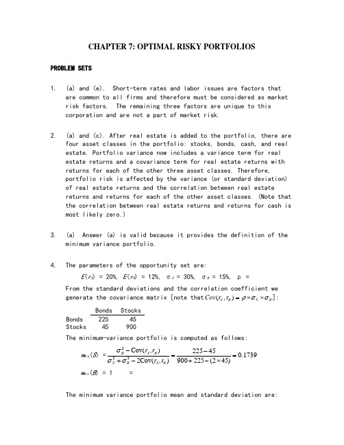
CHAPTER 7: OPTIMAL RISKY PORTFOLIOSPROBLEM SETS1. (a) and (e). Short-term rates and labor issues are factors thatare common to all firms and therefore must be considered as market risk factors. The remaining three factors are unique to this corporation and are not a part of market risk.2. (a) and (c). After real estate is added to the portfolio, there arefour asset classes in the portfolio: stocks, bonds, cash, and real estate. Portfolio variance now includes a variance term for real estate returns and a covariance term for real estate returns with returns for each of the other three asset classes. Therefore,portfolio risk is affected by the variance (or standard deviation) of real estate returns and the correlation between real estatereturns and returns for each of the other asset classes. (Note that the correlation between real estate returns and returns for cash is most likely zero.)3. (a) Answer (a) is valid because it provides the definition of theminimum variance portfolio.4. The parameters of the opportunity set are:E (r S ) = 20%, E (r B ) = 12%, σS = 30%, σB = 15%, ρ =From the standard deviations and the correlation coefficient we generate the covariance matrix [note that (,)S B S B Cov r r ρσσ=⨯⨯]: Bonds Stocks Bonds 225 45 Stocks 45 900The minimum-variance portfolio is computed as follows:w Min (S ) =1739.0)452(22590045225)(Cov 2)(Cov 222=⨯-+-=-+-B S B S B S B ,r r ,r r σσσ w Min (B ) = 1 =The minimum variance portfolio mean and standard deviation are:E (r Min ) = × .20) + × .12) = .1339 = %σMin = 2/12222)],(Cov 2[B S B S B B S Sr r w w w w ++σσ = [ 900) + 225) + (2 45)]1/2= %5.Proportion in Stock Fund Proportionin Bond Fund ExpectedReturnStandard Deviation% % % %minimumtangencyGraph shown below.0.005.0010.0015.0020.0025.000.00 5.00 10.00 15.00 20.00 25.00 30.00Tangency PortfolioMinimum Variance PortfolioEfficient frontier of risky assetsCMLINVESTMENT OPPORTUNITY SETr f = 8.006. The above graph indicates that the optimal portfolio is thetangency portfolio with expected return approximately % andstandard deviation approximately %.7. The proportion of the optimal risky portfolio invested in the stockfund is given by:222[()][()](,)[()][()][()()](,)S f B B f S B S S f B B f SS f B f S B E r r E r r Cov r r w E r r E r r E r r E r r Cov r r σσσ-⨯--⨯=-⨯+-⨯--+-⨯[(.20.08)225][(.12.08)45]0.4516[(.20.08)225][(.12.08)900][(.20.08.12.08)45]-⨯--⨯==-⨯+-⨯--+-⨯10.45160.5484B w =-=The mean and standard deviation of the optimal risky portfolio are:E (r P ) = × .20) + × .12) = .1561 = % σp = [ 900) +225) + (2× 45)]1/2= %8. The reward-to-volatility ratio of the optimal CAL is:().1561.080.4601.1654p fpE r r σ--==9. a. If you require that your portfolio yield an expected return of14%, then you can find the corresponding standard deviation from the optimal CAL. The equation for this CAL is:()().080.4601p fC f C C PE r r E r r σσσ-=+=+If E (r C ) is equal to 14%, then the standard deviation of the portfolio is %.b. To find the proportion invested in the T-bill fund, rememberthat the mean of the complete portfolio ., 14%) is an average of the T-bill rate and the optimal combination of stocks and bonds (P ). Let y be the proportion invested in the portfolio P . The mean of any portfolio along the optimal CAL is:()(1)()[()].08(.1561.08)C f P f P f E r y r y E r r y E r r y =-⨯+⨯=+⨯-=+⨯-Setting E (r C ) = 14% we find: y = and (1 − y ) = (the proportion invested in the T-bill fund).To find the proportions invested in each of the funds, multiply times the respective proportions of stocks and bonds in the optimal risky portfolio:Proportion of stocks in complete portfolio = =Proportion of bonds in complete portfolio = =10. Using only the stock and bond funds to achieve a portfolio expectedreturn of 14%, we must find the appropriate proportion in the stock fund (w S) and the appropriate proportion in the bond fund (w B = 1 −w S) as follows:= × w S + × (1 −w S) = + × w S w S =So the proportions are 25% invested in the stock fund and 75% inthe bond fund. The standard deviation of this portfolio will be:σP = [ 900) + 225) + (2 45)]1/2 = %This is considerably greater than the standard deviation of %achieved using T-bills and the optimal portfolio.11. a.Even though it seems that gold is dominated by stocks, gold mightstill be an attractive asset to hold as a part of a portfolio. Ifthe correlation between gold and stocks is sufficiently low, goldwill be held as a component in a portfolio, specifically, theoptimal tangency portfolio.b.If the correlation between gold and stocks equals +1, then no onewould hold gold. The optimal CAL would be composed of bills andstocks only. Since the set of risk/return combinations of stocksand gold would plot as a straight line with a negative slope (seethe following graph), these combinations would be dominated bythe stock portfolio. Of course, this situation could not persist.If no one desired gold, its price would fall and its expectedrate of return would increase until it became sufficientlyattractive to include in a portfolio.12. Since Stock A and Stock B are perfectly negatively correlated, arisk-free portfolio can be created and the rate of return for thisportfolio, in equilibrium, will be the risk-free rate. To find theproportions of this portfolio [with the proportion w A invested inStock A and w B = (1 –w A) invested in Stock B], set the standarddeviation equal to zero. With perfect negative correlation, theportfolio standard deviation is:σP = Absolute value [w AσA w BσB]0 = 5 × w A− [10 (1 –w A)] w A =The expected rate of return for this risk-free portfolio is:E(r) = × 10) + × 15) = %Therefore, the risk-free rate is: %13. False. If the borrowing and lending rates are not identical, then,depending on the tastes of the individuals (that is, the shape oftheir indifference curves), borrowers and lenders could havedifferent optimal risky portfolios.14. False. The portfolio standard deviation equals the weighted averageof the component-asset standard deviations only in the special case that all assets are perfectly positively correlated. Otherwise, as the formula for portfolio standard deviation shows, the portfoliostandard deviation is less than the weighted average of thecomponent-asset standard deviations. The portfolio variance is aweighted sum of the elements in the covariance matrix, with theproducts of the portfolio proportions as weights.15. The probability distribution is:Probability Rate ofReturn100%−50Mean = [ × 100%] + [ × (-50%)] = 55%Variance = [ × (100 − 55)2] + [ × (-50 − 55)2] = 4725Standard deviation = 47251/2 = %16. σP = 30 = y× σ = 40 × y y =E(r P) = 12 + (30 − 12) = %17. The correct choice is (c). Intuitively, we note that since allstocks have the same expected rate of return and standard deviation, we choose the stock that will result in lowest risk. This is thestock that has the lowest correlation with Stock A.More formally, we note that when all stocks have the same expected rate of return, the optimal portfolio for any risk-averse investor is the global minimum variance portfolio (G). When the portfolio is restricted to Stock A and one additional stock, the objective is to find G for any pair that includes Stock A, and then select thecombination with the lowest variance. With two stocks, I and J, theformula for the weights in G is:)(1)(),(Cov 2),(Cov )(222I w J w r r r r I w Min Min J I J I J I J Min -=-+-=σσσSince all standard deviations are equal to 20%:(,)400and ()()0.5I J I J Min Min Cov r r w I w J ρσσρ====This intuitive result is an implication of a property of any efficient frontier, namely, that the covariances of the global minimum variance portfolio with all other assets on the frontier are identical and equal to its own variance. (Otherwise, additional diversification would further reduce the variance.) In this case, the standard deviation of G(I, J) reduces to:1/2()[200(1)]Min IJ G σρ=⨯+This leads to the intuitive result that the desired addition would be the stock with the lowest correlation with Stock A, which is Stock D. The optimal portfolio is equally invested in Stock A and Stock D, and the standard deviation is %.18. No, the answer to Problem 17 would not change, at least as long asinvestors are not risk lovers. Risk neutral investors would not care which portfolio they held since all portfolios have an expected return of 8%.19. Yes, the answers to Problems 17 and 18 would change. The efficientfrontier of risky assets is horizontal at 8%, so the optimal CAL runs from the risk-free rate through G. This implies risk-averse investors will just hold Treasury bills.20. Rearrange the table (converting rows to columns) and compute serialcorrelation results in the following table:Nominal RatesFor example: to compute serial correlation in decade nominalreturns for large-company stocks, we set up the following twocolumns in an Excel spreadsheet. Then, use the Excel function“CORREL” to calculate the correlation for the data.Decade Previous1930s%%1940s%%1950s%%1960s%%1970s%%1980s%%1990s%%Note that each correlation is based on only seven observations, so we cannot arrive at any statistically significant conclusions.Looking at the results, however, it appears that, with theexception of large-company stocks, there is persistent serialcorrelation. (This conclusion changes when we turn to real rates in the next problem.)21. The table for real rates (using the approximation of subtracting adecade’s average inflation from the decade’s average nominalreturn) is:Real RatesSmall Company StocksLarge Company StocksLong-TermGovernmentBondsIntermed-TermGovernmentBondsTreasuryBills 1920s1930s1940s1950s1960s1970s1980s1990sSerialCorrelationWhile the serial correlation in decade nominal returns seems to be positive, it appears that real rates are serially uncorrelated. The decade time series (although again too short for any definitiveconclusions) suggest that real rates of return are independent from decade to decade.22. The 3-year risk premium for the S&P portfolio is, the 3-year risk premium for thehedge fund portfolio is S&P 3-year standard deviation is 0. The hedge fund 3-year standard deviation is 0. S&P Sharpe ratio is = , and the hedge fund Sharpe ratio is = .23. With a ρ = 0, the optimal asset allocation is,.With these weights,EThe resulting Sharpe ratio is = . Greta has a risk aversion of A=3, Therefore, she will investyof her wealth in this risky portfolio. The resulting investment composition will be S&P: = % and Hedge: = %. The remaining 26% will be invested in the risk-free asset.24. With ρ = , the annual covariance is .25. S&P 3-year standard deviation is . The hedge fund 3-year standard deviation is . Therefore, the 3-year covariance is 0.26. With a ρ=.3, the optimal asset allocation is, .With these weights,E. The resulting Sharpe ratio is = . Notice that the higher covariance results in a poorer Sharpe ratio.Greta will investyof her wealth in this risky portfolio. The resulting investment composition will be S&P: =% and hedge: = %. The remaining % will be invested in the risk-free asset.CFA PROBLEMS1. a. Restricting the portfolio to 20 stocks, rather than 40 to 50stocks, will increase the risk of the portfolio, but it ispossible that the increase in risk will be minimal. Suppose that, for instance, the 50 stocks in a universe have the same standard deviation () and the correlations between each pair areidentical, with correlation coefficient ρ. Then, the covariance between each pair of stocks would be ρσ2, and the variance of an equally weighted portfolio would be:222ρσ1σ1σnn n P -+=The effect of the reduction in n on the second term on theright-hand side would be relatively small (since 49/50 is close to 19/20 and ρσ2 is smaller than σ2), but thedenominator of the first term would be 20 instead of 50. For example, if σ = 45% and ρ = , then the standard deviation with 50 stocks would be %, and would rise to % when only 20 stocks are held. Such an increase might be acceptable if the expected return is increased sufficiently.b. Hennessy could contain the increase in risk by making sure thathe maintains reasonable diversification among the 20 stocks that remain in his portfolio. This entails maintaining a low correlation among the remaining stocks. For example, in part (a), with ρ = , the increase in portfolio risk was minimal. As a practical matter, this means that Hennessy would have to spread his portfolio among many industries; concentrating on just a few industries would result in higher correlations among the included stocks.2. Risk reduction benefits from diversification are not a linearfunction of the number of issues in the portfolio. Rather, the incremental benefits from additional diversification are mostimportant when you are least diversified. Restricting Hennessy to 10 instead of 20 issues would increase the risk of his portfolio by a greater amount than would a reduction in the size of theportfolio from 30 to 20 stocks. In our example, restricting the number of stocks to 10 will increase the standard deviation to %. The % increase in standard deviation resulting from giving up 10 of20 stocks is greater than the % increase that results from givingup 30 of 50 stocks.3. The point is well taken because the committee should be concernedwith the volatility of the entire portfolio. Since Hennessy’sportfolio is only one of six well-diversified portfolios and issmaller than the average, the concentration in fewer issues mighthave a minimal effect on the diversification of the total fund.Hence, unleashing Hennessy to do stock picking may be advantageous.4. d. Portfolio Y cannot be efficient because it is dominated byanother portfolio. For example, Portfolio X has both higherexpected return and lower standard deviation.5. c.6. d.7. b.8. a.9. c.10. Since we do not have any information about expected returns, wefocus exclusively on reducing variability. Stocks A and C have equal standard deviations, but the correlation of Stock B with Stock C is less than that of Stock A with Stock B . Therefore, a portfoliocomposed of Stocks B and C will have lower total risk than aportfolio composed of Stocks A and B.11. Fund D represents the single best addition to complementStephenson's current portfolio, given his selection criteria. Fund D’s expected return percent) has the potential to increase theportfolio’s return somewhat. Fund D’s relatively low correlation with his current portfolio (+ indicates that Fund D will providegreater diversification benefits than any of the other alternativesexcept Fund B. The result of adding Fund D should be a portfolio with approximately the same expected return and somewhat lower volatility compared to the original portfolio.The other three funds have shortcomings in terms of expected return enhancement or volatility reduction through diversification. Fund A offers the potential for increasing the portfolio’s return but is too highly correlated to provide substantial volatility reduction benefits through diversification. Fund B provides substantial volatility reduction through diversification benefits but is expected to generate a return well below the current portfolio’s return. Fund C has the greatest potential to increase the portfolio’s return but is too highly correlated with the current portfolio to provide substantial volatility reduction benefits through diversification.12. a. Subscript OP refers to the original portfolio, ABC to thenew stock, and NP to the new portfolio.i. E(r NP) = w OP E(r OP) + w ABC E(r ABC) = + = %ii. Cov = ρOP ABC = =iii. NP = [w OP2OP2 + w ABC2ABC2 + 2 w OP w ABC(Cov OP , ABC)]1/2= [ 2 + + (2 ]1/2= % %b. Subscript OP refers to the original portfolio, GS to governmentsecurities, and NP to the new portfolio.i. E(r NP) = w OP E(r OP) + w GS E(r GS) = + = %ii. Cov = ρOP GS = 0 0 = 0iii. NP = [w OP2OP2 + w GS2GS2 + 2 w OP w GS (Cov OP , GS)]1/2= [ + 0) + (2 0)]1/2= % %c. Adding the risk-free government securities would result in alower beta for the new portfolio. The new portfolio beta will bea weighted average of the individual security betas in theportfolio; the presence of the risk-free securities would lowerthat weighted average.d. The comment is not correct. Although the respective standarddeviations and expected returns for the two securities underconsideration are equal, the covariances between each security andthe original portfolio are unknown, making it impossible to drawthe conclusion stated. For instance, if the covariances aredifferent, selecting one security over the other may result in alower standard deviation for the portfolio as a whole. In such acase, that security would be the preferred investment, assumingall other factors are equal.e. i. Grace clearly expressed the sentiment that the risk of losswas more important to her than the opportunity for return. Usingvariance (or standard deviation) as a measure of risk in her casehas a serious limitation because standard deviation does notdistinguish between positive and negative price movements.ii. Two alternative risk measures that could be used instead ofvariance are:Range of returns, which considers the highest and lowestexpected returns in the future period, with a larger rangebeing a sign of greater variability and therefore of greaterrisk.Semivariance can be used to measure expected deviations ofreturns below the mean, or some other benchmark, such as zero.Either of these measures would potentially be superior tovariance for Grace. Range of returns would help to highlightthe full spectrum of risk she is assuming, especially thedownside portion of the range about which she is so concerned.Semivariance would also be effective, because it implicitlyassumes that the investor wants to minimize the likelihood ofreturns falling below some target rate; in Grace’s case, thetarget rate would be set at zero (to protect against negativereturns).13. a. Systematic risk refers to fluctuations in asset prices causedby macroeconomic factors that are common to all risky assets;hence systematic risk is often referred to as market risk.Examples of systematic risk factors include the business cycle,inflation, monetary policy, fiscal policy, and technologicalchanges.Firm-specific risk refers to fluctuations in asset pricescaused by factors that are independent of the market, such asindustry characteristics or firm characteristics. Examples offirm-specific risk factors include litigation, patents,management, operating cash flow changes, and financial leverage.b. Trudy should explain to the client that picking only the topfive best ideas would most likely result in the client holdinga much more risky portfolio. The total risk of a portfolio, orportfolio variance, is the combination of systematic risk andfirm-specific risk.The systematic component depends on the sensitivity of theindividual assets to market movements as measured by beta.Assuming the portfolio is well diversified, the number ofassets will not affect the systematic risk component ofportfolio variance. The portfolio beta depends on theindividual security betas and the portfolio weights of those securities.On the other hand, the components of firm-specific risk (sometimes called nonsystematic risk) are not perfectly positively correlated with each other and, as more assets are added to the portfolio, those additional assets tend to reduce portfolio risk. Hence, increasing the number of securities in a portfolio reduces firm-specific risk. For example, a patent expiration for one company would not affect the othersecurities in the portfolio. An increase in oil prices islikely to cause a drop in the price of an airline stock butwill likely result in an increase in the price of an energy stock. As the number of randomly selected securities increases, the total risk (variance) of the portfolio approaches its systematic variance.。
博迪《投资学》(第10版)笔记和课后习题详解答案
博迪《投资学》(第10版)笔记和课后习题详解答案博迪《投资学》(第10版)笔记和课后习题详解完整版>精研学习?>无偿试用20%资料全国547所院校视频及题库全收集考研全套>视频资料>课后答案>往年真题>职称考试第一部分绪论第1章投资环境1.1复习笔记1.2课后习题详解第2章资产类别与金融工具2.1复习笔记2.2课后习题详解第3章证券是如何交易的3.1复习笔记3.2课后习题详解第4章共同基金与其他投资公司4.1复习笔记4.2课后习题详解第二部分资产组合理论与实践第5章风险与收益入门及历史回顾5.1复习笔记5.2课后习题详解第6章风险资产配置6.1复习笔记6.2课后习题详解第7章最优风险资产组合7.1复习笔记7.2课后习题详解第8章指数模型8.2课后习题详解第三部分资本市场均衡第9章资本资产定价模型9.1复习笔记9.2课后习题详解第10章套利定价理论与风险收益多因素模型10.1复习笔记10.2课后习题详解第11章有效市场假说11.1复习笔记11.2课后习题详解第12章行为金融与技术分析12.1复习笔记12.2课后习题详解第13章证券收益的实证证据13.1复习笔记13.2课后习题详解第四部分固定收益证券第14章债券的价格与收益14.1复习笔记14.2课后习题详解第15章利率的期限结构15.1复习笔记15.2课后习题详解第16章债券资产组合管理16.1复习笔记16.2课后习题详解第五部分证券分析第17章宏观经济分析与行业分析17.2课后习题详解第18章权益估值模型18.1复习笔记18.2课后习题详解第19章财务报表分析19.1复习笔记19.2课后习题详解第六部分期权、期货与其他衍生证券第20章期权市场介绍20.1复习笔记20.2课后习题详解第21章期权定价21.1复习笔记21.2课后习题详解第22章期货市场22.1复习笔记22.2课后习题详解第23章期货、互换与风险管理23.1复习笔记23.2课后习题详解第七部分应用投资组合管理第24章投资组合业绩评价24.1复习笔记24.2课后习题详解第25章投资的国际分散化25.1复习笔记25.2课后习题详解第26章对冲基金26.1复习笔记26.2课后习题详解第27章积极型投资组合管理理论27.1复习笔记27.2课后习题详解第28章投资政策与特许金融分析师协会结构28.1复习笔记28.2课后习题详解。
投资学10版习题答案

CHAPTER 14: BOND PRICES AND YIELDSPROBLEM SETS1. a. Catastrophe bond—A bond that allows the issuer to transfer“catastrophe risk” from the firm to the capital markets. Investors inthese bonds receive a compensation for taking on the risk in the form ofhigher coupon rates. In the event of a catastrophe, the bondholders willreceive only part or perhaps none of the principal payment due to themat maturity. Disaster can be defined by total insured losses or by criteriasuch as wind speed in a hurricane or Richter level in an earthquake.b. Eurobond—A bond that is denominated in one currency, usually thatof the issuer, but sold in other national markets.c. Zero-coupon bond—A bond that makes no coupon payments. Investorsreceive par value at the maturity date but receive no interest paymentsuntil then. These bonds are issued at prices below par value, and theinvestor’s return comes from the difference between issue price and thepayment of par value at maturity (capital gain).d. Samurai bond—Yen-dominated bonds sold in Japan by non-Japaneseissuers.e. Junk bond—A bond with a low credit rating due to its high default risk;also known as high-yield bonds.f. Convertible bond—A bond that gives the bondholders an option toexchange the bond for a specified number of shares of common stock ofthe firm.g. Serial bonds—Bonds issued with staggered maturity dates. As bondsmature sequentially, the principal repayment burden for the firm isspread over time.h. Equipment obligation bond—A collateralized bond for which thecollateral is equipment owned by the firm. If the firm defaults on thebond, the bondholders would receive the equipment.i. Original issue discount bond—A bond issued at a discount to the facevalue.j. Indexed bond— A bond that makes payments that are tied to ageneral price index or the price of a particular commodity.k. Callable bond—A bond that gives the issuer the option to repurchase the bond at a specified call price before the maturity date.l. Puttable bond —A bond that gives the bondholder the option to sell back the bond at a specified put price before the maturity date.2. The bond callable at 105 should sell at a lower price because the call provision is more valuable to the firm. Therefore, its yield to maturity should be higher.3.Zero coupon bonds provide no coupons to be reinvested. Therefore, the investor's proceeds from the bond are independent of the rate at which coupons could be reinvested (if they were paid). There is no reinvestment rate uncertainty with zeros.4.A bond’s coupon interest payments and principal repayment are not affected by changes in market rates. Consequently, if market ratesincrease, bond investors in the secondary markets are not willing to pay as much for a claim on a gi ven bond’s fixed interest and principalpayments as they would if market rates were lower. This relationship is apparent from the inverse relationship between interest rates and present value. An increase in the discount rate (i.e., the market rate. decreases the present value of the future cash flows. 5. Annual coupon rate: 4.80% $48 Coupon paymentsCurrent yield:$48 4.95%$970⎛⎫= ⎪⎝⎭6. a.Effective annual rate for 3-month T-bill:%0.10100.0102412.11645,97000,10044==-=-⎪⎭⎫ ⎝⎛b. Effective annual interest rate for coupon bond paying 5% semiannually:(1.05.2—1 = 0.1025 or 10.25%Therefore the coupon bond has the higher effective annual interest rate. 7.The effective annual yield on the semiannual coupon bonds is 8.16%. If the annual coupon bonds are to sell at par they must offer the same yield, which requires an annual coupon rate of 8.16%.8. The bond price will be lower. As time passes, the bond price, which isnow above par value, will approach par.9. Yield to maturity: Using a financial calculator, enter the following:n = 3; PV = -953.10; FV = 1000; PMT = 80; COMP iThis results in: YTM = 9.88%Realized compound yield: First, find the future value (FV. of reinvestedcoupons and principal:FV = ($80 * 1.10 *1.12. + ($80 * 1.12. + $1,080 = $1,268.16Then find the rate (y realized . that makes the FV of the purchase price equal to $1,268.16:$953.10 ⨯ (1 + y realized .3 = $1,268.16 ⇒y realized = 9.99% or approximately 10% Using a financial calculator, enter the following: N = 3; PV = -953.10; FV =1,268.16; PMT = 0; COMP I. Answer is 9.99%.10.a. Zero coupon 8%10% couponcouponCurrent prices $463.19 $1,000.00 $1,134.20b. Price 1 year from now $500.25 $1,000.00 $1,124.94Price increase $ 37.06 $ 0.00 − $ 9.26Coupon income $ 0.00 $ 80.00 $100.00Pretax income $ 37.06 $ 80.00 $ 90.74Pretax rate of return 8.00% 8.00% 8.00%Taxes* $ 11.12 $ 24.00 $ 28.15After-tax income $ 25.94 $ 56.00 $ 62.59After-tax rate of return 5.60% 5.60% 5.52%c. Price 1 year from now $543.93 $1,065.15 $1,195.46Price increase $ 80.74 $ 65.15 $ 61.26Coupon income $ 0.00 $ 80.00 $100.00Pretax income $ 80.74 $145.15 $161.26Pretax rate of return 17.43% 14.52% 14.22%Taxes†$ 19.86 $ 37.03 $ 42.25After-tax income $ 60.88 $108.12 $119.01After-tax rate of return 13.14% 10.81% 10.49%* In computing taxes, we assume that the 10% coupon bond was issued at par and that the decrease in price when the bond is sold at year-end is treated as a capital loss and therefore is not treated as an offset to ordinary income.† In computing taxes for the zero coupon bond, $37.06 is taxed as ordinary income (see part (b); the remainder of the price increase is taxed as a capital gain.11. a. On a financial calculator, enter the following:n = 40; FV = 1000; PV = –950; PMT = 40You will find that the yield to maturity on a semiannual basis is 4.26%.This implies a bond equivalent yield to maturity equal to: 4.26% * 2 =8.52%Effective annual yield to maturity = (1.0426)2– 1 = 0.0870 = 8.70%b. Since the bond is selling at par, the yield to maturity on a semiannualbasis is the same as the semiannual coupon rate, i.e., 4%. The bondequivalent yield to maturity is 8%.Effective annual yield to maturity = (1.04)2– 1 = 0.0816 = 8.16%c. Keeping other inputs unchanged but setting PV = –1050, we find abond equivalent yield to maturity of 7.52%, or 3.76% on a semiannualbasis.Effective annual yield to maturity = (1.0376)2– 1 = 0.0766 = 7.66%12. Since the bond payments are now made annually instead of semiannually,the bond equivalent yield to maturity is the same as the effective annual yield to maturity. [On a financial calculator, n = 20; FV = 1000; PV = –price; PMT = 80]The resulting yields for the three bonds are:Bond Price Bond Equivalent Yield= Effective Annual Yield$950 8.53%1,000 8.001,050 7.51The yields computed in this case are lower than the yields calculatedwith semiannual payments. All else equal, bonds with annual payments are less attractive to investors because more time elapses beforepayments are received. If the bond price is the same with annualpayments, then the bond's yield to maturity is lower.13.Price Maturity(years.BondEquivalentYTM$400.00 20.00 4.688% 500.00 20.00 3.526 500.00 10.00 7.177385.54 10.00 10.000 463.19 10.00 8.000 400.00 11.91 8.00014. a. The bond pays $50 every 6 months. The current price is:[$50 × Annuity factor (4%, 6)] + [$1,000 × PV factor (4%, 6)] = $1,052.42 Alternatively, PMT = $50; FV = $1,000; I = 4; N = 6. Solve for PV = $1,052.42.If the market interest rate remains 4% per half year, price six months from now is:[$50 × Annuity factor (4%, 5)] + [$1,000 × PV factor (4%, 5)] = $1,044.52Alternatively, PMT = $50; FV = $1,000; I = 4; N = 5. Solve for PV = $1,044.52.b. Rate of return $50($1,044.52$1,052.42)$50$7.904.0%$1,052.42$1,052.42+--===15.The reported bond price is: $1,001.250However, 15 days have passed since the last semiannual coupon was paid, so:Accrued interest = $35 * (15/182) = $2.885The invoice price is the reported price plus accrued interest: $1,004.1416. If the yield to maturity is greater than the current yield, then the bond offers the prospect of price appreciation as it approaches its maturity date. Therefore, the bond must be selling below par value.17. The coupon rate is less than 9%. If coupon divided by price equals 9%, and price is less than par, then price divided by par is less than 9%.18.Time Inflation in YearJust EndedPar Value Coupon Payment Principal Repayment 0 $1,000.001 2% 1,020.00 $40.80 $ 0.002 3% $1,050.60 $42.02 $ 0.00 31%$1,061.11$42.44$1,061.11The nominal rate of return and real rate of return on the bond in each year are computed as follows:Nominal rate of return = interest + price appreciationinitial priceReal rate of return = 1 + nominal return1 + inflation - 1Second YearThird YearNominal return 071196.0020,1$60.30$02.42$=+050400.060.050,1$51.10$44.42$=+Real return%0.4040.0103.1071196.1==- %0.4040.0101.1050400.1==- The real rate of return in each year is precisely the 4% real yield on the bond.19.The price schedule is as follows: Year Remaining Maturity (T).Constant Yield Value $1,000/(1.08)TImputed Interest (increase inconstant yield value)0 (now) 20 years$214.551 19 231.71 $17.162 18 250.25 18.54 19 1 925.93 201,000.0074.0720.The bond is issued at a price of $800. Therefore, its yield to maturity is: 6.8245%Therefore, using the constant yield method, we find that the price in one year (when maturity falls to 9 years) will be (at an unchanged yield. $814.60, representing an increase of $14.60. Total taxable income is: $40.00 + $14.60 = $54.6021. a. The bond sells for $1,124.72 based on the 3.5% yield to maturity .[n = 60; i = 3.5; FV = 1000; PMT = 40]Therefore, yield to call is 3.368% semiannually, 6.736% annually. [n = 10 semiannual periods; PV = –1124.72; FV = 1100; PMT = 40]b. If the call price were $1,050, we would set FV = 1,050 and redo part (a) to find that yield to call is 2.976% semiannually, 5.952% annually. With a lower call price, the yield to call is lower.c. Yield to call is 3.031% semiannually, 6.062% annually. [n = 4; PV = −1124.72; FV = 1100; PMT = 40]22. The stated yield to maturity, based on promised payments, equals 16.075%.[n = 10; PV = –900; FV = 1000; PMT = 140]Based on expected reduced coupon payments of $70 annually, theexpected yield to maturity is 8.526%.23. The bond is selling at par value. Its yield to maturity equals the couponrate, 10%. If the first-year coupon is reinvested at an interest rate of rpercent, then total proceeds at the end of the second year will be: [$100 *(1 + r)] + $1,100Therefore, realized compound yield to maturity is a function of r, as shown in the following table:8% $1,208 1208/1000 – 1 = 0.0991 = 9.91%10% $1,210 1210/1000 – 1 = 0.1000 = 10.00%12% $1,212 1212/1000 – 1 = 0.1009 = 10.09%24. April 15 is midway through the semiannual coupon period. Therefore,the invoice price will be higher than the stated ask price by an amountequal to one-half of the semiannual coupon. The ask price is 101.25percent of par, so the invoice price is:$1,012.50 + (½*$50) = $1,037.5025. Factors that might make the ABC debt more attractive to investors,therefore justifying a lower coupon rate and yield to maturity, are:i. The ABC debt is a larger issue and therefore may sell with greaterliquidity.ii. An option to extend the term from 10 years to 20 years is favorable ifinterest rates 10 years from now are lower than today’s interest rates. Incontrast, if interest rates increase, the investor can present the bond forpayment and reinvest the money for a higher return.iii. In the event of trouble, the ABC debt is a more senior claim. It hasmore underlying security in the form of a first claim against realproperty.iv. The call feature on the XYZ bonds makes the ABC bonds relativelymore attractive since ABC bonds cannot be called from the investor.v. The XYZ bond has a sinking fund requiring XYZ to retire part of theissue each year. Since most sinking funds give the firm the option toretire this amount at the lower of par or market value, the sinking fundcan be detrimental for bondholders.26. A. If an investor believes the firm’s credit prospects are poor in the nearterm and wishes to capitalize on this, the investor should buy a creditdefault swap. Although a short sale of a bond could accomplish the same objective, liquidity is often greater in the swap market than it is in theunderlying cash market. The investor could pick a swap with a maturitysimilar to the expected time horizon of the credit risk. By buying theswap, the investor would receive compensation if the bond experiencesan increase in credit risk.27. a. When credit risk increases, credit default swaps increase in valuebecause the protection they provide is more valuable. Credit defaultswaps do not provide protection against interest rate risk however.28. a. An increase in the firm’s times interest-earned ratio decreases thedefault risk of the firm→increases the bond’s price → decreases the YTM.b. An increase in the issuing firm’s debt-equity ratio increases thedefault risk of the firm → decreases the bond’s price → increases YTM.c. An increase in the issuing firm’s quick ratio increases short-runliquidity, → implying a decrease in default risk of the firm → increasesthe bond’s price → decreases YTM.29. a. The floating rate note pays a coupon that adjusts to market levels.Therefore, it will not experience dramatic price changes as marketyields fluctuate. The fixed rate note will therefore have a greater pricerange.b. Floating rate notes may not sell at par for any of several reasons:(i) The yield spread between one-year Treasury bills and othermoney market instruments of comparable maturity could be wider(or narrower. than when the bond was issued.(ii) The credit standing of the firm may have eroded (or improved.relative to Treasury securities, which have no credit risk.Therefore, the 2% premium would become insufficient to sustainthe issue at par.(iii) The coupon increases are implemented with a lag, i.e., onceevery year. During a period of changing interest rates, even thisbrief lag will be reflected in the price of the security.c. The risk of call is low. Because the bond will almost surely not sell for much above par value (given its adjustable coupon rate), it is unlikely that the bond will ever be called.d. The fixed-rate note currently sells at only 88% of the call price, so that yield to maturity is greater than the coupon rate. Call risk iscurrently low, since yields would need to fall substantially for the firm to use its option to call the bond.e. The 9% coupon notes currently have a remaining maturity of 15 years and sell at a yield to maturity of 9.9%. This is the coupon rate thatwould be needed for a newly issued 15-year maturity bond to sell at par.f. Because the floating rate note pays a variable stream of interestpayments to maturity, the effective maturity for comparative purposes with other debt securities is closer to the next coupon reset date than the final maturity date. Therefore, yield-to-maturity is anindeterminable calculation for a floating rate note, with “yield -to-recoupon date” a more meaningful measure of return.30. a. The yield to maturity on the par bond equals its coupon rate, 8.75%.All else equal, the 4% coupon bond would be more attractive because its coupon rate is far below current market yields, and its price is far below the call price. Therefore, if yields fall, capital gains on the bond will not be limited by the call price. In contrast, the 8¾% coupon bond canincrease in value to at most $1,050, offering a maximum possible gain of only 0.5%. The disadvantage of the 8¾% coupon bond, in terms ofvulnerability to being called, shows up in its higher promised yield to maturity.b. If an investor expects yields to fall substantially, the 4% bond offers a greater expected return.c. Implicit call protection is offered in the sense that any likely fallin yields would not be nearly enough to make the firm considercalling the bond. In this sense, the call feature is almost irrelevant.31. a. Initial price P 0 = $705.46 [n = 20; PMT = 50; FV = 1000; i = 8]Next year's price P 1 = $793.29 [n = 19; PMT = 50; FV = 1000; i = 7] HPR %54.191954.046.705$)46.705$29.793($50$==-+=b. Using OID tax rules, the cost basis and imputed interest under theconstant yield method are obtained by discounting bond payments at the original 8% yield and simply reducing maturity by one year at a time: Constant yield prices (compare these to actual prices to compute capital gains.: P 0 = $705.46P 1 = $711.89 ⇒ implicit interest over first year = $6.43P 2 = $718.84 ⇒ implicit interest over second year = $6.95Tax on explicit interest plus implicit interest in first year =0.40*($50 + $6.43) = $22.57Capital gain in first year = Actual price at 7% YTM —constant yield price =$793.29—$711.89 = $81.40Tax on capital gain = 0.30*$81.40 = $24.42Total taxes = $22.57 + $24.42 = $46.99c. After tax HPR =%88.121288.046.705$99.46$)46.705$29.793($50$==--+d. Value of bond after two years = $798.82 [using n = 18; i = 7%; PMT = $50; FV = $1,000]Reinvested income from the coupon interest payments = $50*1.03 + $50 = $101.50Total funds after two years = $798.82 + $101.50 = $900.32Therefore, the investment of $705.46 grows to $900.32 in two years:$705.46 (1 + r )2 = $900.32 ⇒ r = 0.1297 = 12.97%e. Coupon interest received in first year: $50.00Less: tax on coupon interest 40%: – 20.00Less: tax on imputed interest (0.40*$6.43): – 2.57Net cash flow in first year: $27.43The year-1 cash flow can be invested at an after-tax rate of:3% × (1 – 0.40) = 1.8%By year 2, this investment will grow to: $27.43 × 1.018 = $27.92In two years, sell the bond for: $798.82 [n = 18; i = 7%%; PMT =$50; FV = $1,000]Less: tax on imputed interest in second year:– 2.78 [0.40 × $6.95] Add: after-tax coupon interest received in second year: + 30.00 [$50 × (1 – 0.40)]Less: Capital gains tax on(sales price – constant yield value): – 23.99 [0.30 × (798.82 – 718.84)] Add: CF from first year's coupon (reinvested):+ 27.92 [from above]Total $829.97$705.46 (1 + r)2 = $829.97 r = 0.0847 = 8.47%CFA PROBLEMS1. a. A sinking fund provision requires the early redemption of a bond issue.The provision may be for a specific number of bonds or a percentage ofthe bond issue over a specified time period. The sinking fund can retireall or a portion of an issue over the life of the issue.b. (i) Compared to a bond without a sinking fund, the sinking fundreduces the average life of the overall issue because some of thebonds are retired prior to the stated maturity.(ii) The company will make the same total principal payments overthe life of the issue, although the timing of these payments will beaffected. The total interest payments associated with the issue willbe reduced given the early redemption of principal.c. From the investor’s point of view, the key reason for demanding asinking fund is to reduce credit risk. Default risk is reduced by theorderly retirement of the issue.2. a. (i) Current yield = Coupon/Price = $70/$960 = 0.0729 = 7.29%(ii) YTM = 3.993% semiannually, or 7.986% annual bond equivalent yield.On a financial calculator, enter: n = 10; PV = –960; FV = 1000; PMT = 35Compute the interest rate.(iii) Realized compound yield is 4.166% (semiannually), or 8.332% annualbond equivalent yield. To obtain this value, first find the future value(FV) of reinvested coupons and principal. There will be six payments of$35 each, reinvested semiannually at 3% per period. On a financialcalculator, enter:PV = 0; PMT = 35; n = 6; i = 3%. Compute: FV = 226.39Three years from now, the bond will be selling at the par value of $1,000because the yield to maturity is forecast to equal the coupon rate.Therefore, total proceeds in three years will be: $226.39 + $1,000 =$1,226.39Then find the rate (y realized. that makes the FV of the purchaseprice equal to $1,226.39:$960 × (1 + y realized.6 = $1,226.39 y realized = 4.166% (semiannual.Alternatively, PV = −$960; FV = $1,226.39; N = 6; PMT = $0. Solve for I =4.16%.b. Shortcomings of each measure:(i) Current yield does not account for capital gains or losses on bondsbought at prices other than par value. It also does not account forreinvestment income on coupon payments.(ii) Yield to maturity assumes the bond is held until maturity and that all coupon income can be reinvested at a rate equal to the yield to maturity.(iii) Realized compound yield is affected by the forecast ofreinvestment rates, holding period, and yield of the bond at the endof the investor's holding period.3. a. The maturity of each bond is 10 years, and we assume that couponsare paid semiannually. Since both bonds are selling at par value, thecurrent yield for each bond is equal to its coupon rate.If the yield declines by 1% to 5% (2.5% semiannual yield., the Sentinalbond will increase in value to $107.79 [n=20; i = 2.5%; FV = 100; PMT = 3].The price of the Colina bond will increase, but only to the call price of102. The present value of scheduled payments is greater than 102, butthe call price puts a ceiling on the actual bond price.b. If rates are expected to fall, the Sentinal bond is more attractive:since it is not subject to call, its potential capital gains are greater.If rates are expected to rise, Colina is a relatively better investment. Itshigher coupon (which presumably is compensation to investors for thecall feature of the bond. will provide a higher rate of return than theSentinal bond.c. An increase in the volatility of rates will increase the value of thefirm’s option to call back the Colina bond. If rates go down, the firm can call the bond, which puts a cap on possible capital gains. So, greatervolatility makes the option to call back the bond more valuable to theissuer. This makes the bond less attractive to the investor.4. Market conversion value = Value if converted into stock = 20.83 × $28 =$583.24Conversion premium = Bond price – Market conversion value= $775.00 – $583.24 = $191.765. a. The call feature requires the firm to offer a higher coupon (or higherpromised yield to maturity) on the bond in order to compensate theinvestor for the firm's option to call back the bond at a specified priceif interest rate falls sufficiently. Investors are willing to grant thisvaluable option to the issuer, but only for a price that reflects thepossibility that the bond will be called. That price is the higherpromised yield at which they are willing to buy the bond.b. The call feature reduces the expected life of the bond. If interestrates fall substantially so that the likelihood of a call increases,investors will treat the bond as if it will "mature" and be paid off at thecall date, not at the stated maturity date. On the other hand, if ratesrise, the bond must be paid off at the maturity date, not later. Thisasymmetry means that the expected life of the bond is less than thestated maturity.c. The advantage of a callable bond is the higher coupon (and higherpromised yield to maturity) when the bond is issued. If the bond is never called, then an investor earns a higher realized compound yield on acallable bond issued at par than a noncallable bond issued at par on the same date. The disadvantage of the callable bond is the risk of call. Ifrates fall and the bond is called, then the investor receives the call price and then has to reinvest the proceeds at interest rates that are lowerthan the yield to maturity at which the bond originally was issued. Inthis event, the firm's savings in interest payments is the investor's loss.6. a. (iii)b. (iii) The yield to maturity on the callable bond must compensatethe investor for the risk of call.Choice (i) is wrong because, although the owner of a callablebond receives a premium plus the principal in the event of a call,the interest rate at which he can reinvest will be low. The lowinterest rate that makes it profitable for the issuer to call thebond also makes it a bad deal f or the bond’s holder.Choice (ii) is wrong because a bond is more apt to be called wheninterest rates are low. Only if rates are low will there be aninterest saving for the issuer.c. (iii)d. (ii)。
投资学第10版课后习题答案
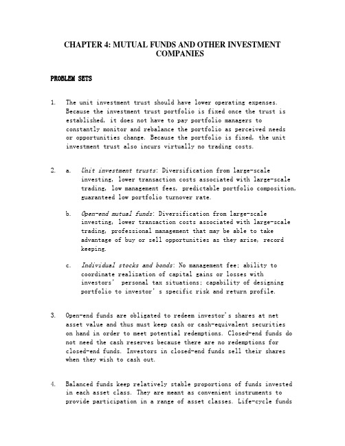
CHAPTER 4: MUTUAL FUNDS AND OTHER INVESTMENTCOMPANIESPROBLEM SETS1. The unit investment trust should have lower operating expenses.Because the investment trust portfolio is fixed once the trust isestablished, it does not have to pay portfolio managers toconstantly monitor and rebalance the portfolio as perceived needsor opportunities change. Because the portfolio is fixed, the unitinvestment trust also incurs virtually no trading costs.2. a. Unit investment trusts: Diversification from large-scaleinvesting, lower transaction costs associated with large-scaletrading, low management fees, predictable portfolio composition,guaranteed low portfolio turnover rate.b. Open-end mutual funds: Diversification from large-scaleinvesting, lower transaction costs associated with large-scaletrading, professional management that may be able to takeadvantage of buy or sell opportunities as they arise, recordkeeping.c. Individual stocks and bonds: No management fee; ability tocoordinate realization of capital gains or losses withinvestors’ personal tax situation s; capability of designingportfolio to investor’s specific risk and return profile.3. Open-end funds are obligated to redeem investor's shares at netasset value and thus must keep cash or cash-equivalent securitieson hand in order to meet potential redemptions. Closed-end funds do not need the cash reserves because there are no redemptions forclosed-end funds. Investors in closed-end funds sell their shareswhen they wish to cash out.4. Balanced funds keep relatively stable proportions of funds investedin each asset class. They are meant as convenient instruments toprovide participation in a range of asset classes. Life-cycle fundsare balanced funds whose asset mix generally depends on the age of the investor. Aggressive life-cycle funds, with larger investments in equities, are marketed to younger investors, while conservative life-cycle funds, with larger investments in fixed-income securities, are designed for older investors. Asset allocation funds, in contrast, may vary the proportions invested in each asset class by large amounts as predictions of relative performance across classes vary. Asset allocation funds therefore engage in more aggressive market timing.5. Unlike an open-end fund, in which underlying shares are redeemedwhen the fund is redeemed, a closed-end fund trades as a security in the market. Thus, their prices may differ from the NAV.6. Advantages of an ETF over a mutual fund:ETFs are continuously traded and can be sold or purchased on margin.There are no capital gains tax triggers when an ETF is sold(shares are just sold from one investor to another).Investors buy from brokers, thus eliminating the cost ofdirect marketing to individual small investors. This implieslower management fees.Disadvantages of an ETF over a mutual fund:Prices can depart from NAV (unlike an open-end fund).There is a broker fee when buying and selling (unlike a no-load fund).7. The offering price includes a 6% front-end load, or salescommission, meaning that every dollar paid results in only $ going toward purchase of shares. Therefore: Offering price =06.0170.10$Load 1NAV -=-= $8. NAV = Offering price (1 –Load) = $ .95 = $9. Stock Value Held by FundA $ 7,000,000B 12,000,000C 8,000,000D 15,000,000Total $42,000,000Net asset value =000,000,4000,30$000,000,42$-= $10. Value of stocks sold and replaced = $15,000,000 Turnover rate =000,000,42$000,000,15$= , or %11. a. 40.39$000,000,5000,000,3$000,000,200$NAV =-=b. Premium (or discount) = NAVNAV ice Pr - = 40.39$40.39$36$-= –, or % The fund sells at an % discount from NAV.12. 100NAV NAV Distributions $12.10$12.50$1.500.088, or 8.8%NAV $12.50-+-+==13. a. Start-of-year price: P 0 = $ × = $End-of-year price: P 1 = $ × = $Although NAV increased by $, the price of the fund decreased by $. Rate of return =100Distributions $11.25$12.24$1.500.042, or 4.2%$12.24P P P -+-+==b. An investor holding the same securities as the fund managerwould have earned a rate of return based on the increase in the NAV of the portfolio:100NAV NAV Distributions $12.10$12.00$1.500.133, or 13.3%NAV $12.00-+-+==14. a. Empirical research indicates that past performance of mutualfunds is not highly predictive of future performance,especially for better-performing funds. While there may be some tendency for the fund to be an above average performer nextyear, it is unlikely to once again be a top 10% performer.b. On the other hand, the evidence is more suggestive of atendency for poor performance to persist. This tendency isprobably related to fund costs and turnover rates. Thus if the fund is among the poorest performers, investors should beconcerned that the poor performance will persist.15. NAV 0 = $200,000,000/10,000,000 = $20Dividends per share = $2,000,000/10,000,000 = $NAV1 is based on the 8% price gain, less the 1% 12b-1 fee: NAV1 = $20 (1 – = $Rate of return =20$20 .0$20$384.21$+-= , or %16. The excess of purchases over sales must be due to new inflows intothe fund. Therefore, $400 million of stock previously held by the fund was replaced by new holdings. So turnover is: $400/$2,200 = , or %.17. Fees paid to investment managers were: $ billion = $ millionSince the total expense ratio was % and the management fee was %, we conclude that % must be for other expenses. Therefore, other administrative expenses were: $ billion = $ million.18. As an initial approximation, your return equals the return on the shares minus the total of the expense ratio and purchase costs: 12% % 4% = %.But the precise return is less than this because the 4% load is paid up front, not at the end of the year. To purchase the shares, you would have had to invest: $20,000/(1 = $20,833. The shares increase in value from $20,000 to: $20,000 = $22,160. The rate of return is: ($22,160 $20,833)/$20,833 = %.19. Assume $1,000 investmentLoaded-Up Fund Economy Fund Yearly growth (r is 6%) (1.01.0075)r +-- (.98)(1.0025)r ⨯+- t = 1 year$1, $1, t = 3 years$1, $1, t = 10 years$1, $1,20. a. $450,000,000$10,000000$1044,000,000-= b. The redemption of 1 million shares will most likely triggercapital gains taxes which will lower the remaining portfolio by an amount greater than $10,000,000 (implying a remaining total value less than $440,000,000). The outstanding shares fall to 43 million and the NAV drops to below $10.21. Suppose you have $1,000 to invest. The initial investment in ClassA shares is $940 net of the front-end load. After four years, yourportfolio will be worth:$940 4 = $1,Class B shares allow you to invest the full $1,000, but yourinvestment performance net of 12b-1 fees will be only %, and you will pay a 1% back-end load fee if you sell after four years. Your portfolio value after four years will be:$1,000 4 = $1,After paying the back-end load fee, your portfolio value will be:$1, .99 = $1,Class B shares are the better choice if your horizon is four years.With a 15-year horizon, the Class A shares will be worth:$940 15 = $3,For the Class B shares, there is no back-end load in this casesince the horizon is greater than five years. Therefore, the value of the Class B shares will be:$1,000 15 = $3,At this longer horizon, Class B shares are no longer the betterchoice. The effect of Class B's % 12b-1 fees accumulates over time and finally overwhelms the 6% load charged to Class A investors.22. a. After two years, each dollar invested in a fund with a 4% loadand a portfolio return equal to r will grow to: $ (1 + r–2.Each dollar invested in the bank CD will grow to: $1 .If the mutual fund is to be the better investment, then theportfolio return (r) must satisfy:(1 + r–2 >(1 + r–2 >(1 + r–2 >1 + r– >1 + r >Therefore: r > = %b. If you invest for six years, then the portfolio return mustsatisfy:(1 + r–6 > =(1 + r–6 >1 + r– >r > %The cutoff rate of return is lower for the six-year investment because the “fixed cost” (the one-time front-end load) is spread over a greater number of years.c. With a 12b-1 fee instead of a front-end load, the portfoliomust earn a rate of return (r ) that satisfies:1 + r – – >In this case, r must exceed % regardless of the investmenthorizon.23. The turnover rate is 50%. This means that, on average, 50% of theportfolio is sold and replaced with other securities each year. Trading costs on the sell orders are % and the buy orders toreplace those securities entail another % in trading costs. Total trading costs will reduce portfolio returns by: 2 % = %24. For the bond fund, the fraction of portfolio income given up tofees is: %0.4%6.0= , or % For the equity fund, the fraction of investment earnings given up to fees is:%0.12%6.0= , or % Fees are a much higher fraction of expected earnings for the bond fund and therefore may be a more important factor in selecting the bond fund.This may help to explain why unmanaged unit investment trusts are concentrated in the fixed income market. The advantages of unit investment trusts are low turnover, low trading costs, and low management fees. This is a more important concern to bond-market investors.25. Suppose that finishing in the top half of all portfolio managers ispurely luck, and that the probability of doing so in any year is exactly ½. Then the probability that any particular manager would finish in the top half of the sample five years in a row is (½)5 = 1/32. We would then expect to find that [350 (1/32)] = 11managers finish in the top half for each of the five consecutiveyears. This is precisely what we found. Thus, we should not conclude that the consistent performance after five years is proof of skill. We would expect to find 11 managers exhibiting precisely this level of "consistency" even if performance is due solely to luck.。
投资学第10章习题及答案

第10章习题及答案1.2008年金融危机对我国股市有何影响?2.货币政策如何影响股市的?3.2008年以来我国实施的宽松的财政政策对于股票市场有何影响?4.简述经济周期与证券市场波动之间的关系?5.影响行业兴衰的因素都有哪些?6.一个公司的行业敏感性取决于哪些因素?参考答案1.国际经济关系对证券市场的影响,包括国际经济的增长状况、国际金融以及利率与汇率的变动、境外股市行情波动、贸易关系等。
其中国际金融以及利率与汇率的变动对于证券市场的影响非常大。
西方主要国际金融市场的利率一旦发生变化,证券市场也会相应的发生变化,即利率的提高将会带来证券市场的下跌趋势,反之利率的降低,证券市场就会上涨。
境外股市行情的波动会立刻影响到我国股市的波动。
一国因为某种因素引发股市危机,就会引发连锁的股市灾难。
另外,贸易关系的改变通常会引起相关国际性公司股票价格发生波动。
如果一国贸易对国际市场依赖性比较大,那么,贸易关系的改善,将会推动该国股市指数的大幅上涨;相反,如果贸易关系恶化,通常会引起该国股市指数的大幅下挫。
例如07年爆发美国次贷危机中,美国股市下跌了55%,以此同时,受到牵连的中国股市跌幅达到73%。
2.从证券投资的角度看, 货币政策可以直接影响证券市场行情。
中央银行的货币政策对证券的价格有重要影响。
从整体来说, 宽松的货币政策将会使证券市场价格上涨;而从紧的货币政策将会使证券市场价格下跌。
货币政策对证券市场的影响可以从四个方面来分析: (1)利率政策对于证券市场价格具有重要影响。
通常证券价格对利率的变动较为敏感。
(2)中央银行的微调政策对证券价格的影响具体表现如下:如果放松银根, 中央银行将大量买进证券, 增加了社会对证券的需求, 引起证券价格上升;如果紧缩银根,中央银行将抛出证券, 使证券供给过旺, 导致价格下跌。
(3)货币政策的综合影响, 当货币供应量过多而造成通货膨胀时, 人们为保值而购买证券(尤其是股票) , 推动证券需求上升, 价格上涨; 当货币供应量不足时, 人们为取得货币资金而抛售证券, 使证券价格下跌。
《投资学》课后习题参考答案

习题参考答案第2章答案:一、选择1、D2、C二、填空1、公众投资者、工商企业投资者、政府2、中国人民保险公司;中国国际信托投资公司3、威尼斯、英格兰4、信用合作社、合作银行;农村信用合作社、城市信用合作社;5、安全性、流动性、效益性三、名词解释:财务公司又称金融公司,是一种经营部分银行业务的非银行金融机构。
其最初是为产业集团内部各分公司筹资,便利集团内部资金融通,但现在经营领域不断扩大,种类不断增加,有的专门经营抵押放款业务,有的专门经营耐用消费品的租购和分期付款业务,大的财务公司还兼营外汇、联合贷款、包销证券、不动产抵押、财务及投资咨询服务等。
信托公司是指以代人理财为主要经营内容、以委托人身份经营现代信托业务的金融机构。
信托公司的业务一般包括货币信托(信托贷款、信托存款、养老金信托、有价证券投资信托等)和非货币信托(债权信托、不动产信托、动产信托等)两大类。
保险公司是一类经营保险业务的金融中介机构。
它以集合多数单位或个人的风险为前提,用其概率计算分摊金,以保险费的形式聚集资金建立保险基金,用于补偿因自然灾害或以外事故造成的经济损失,或对个人因死亡伤残给予物质补偿。
四、简答1、家庭个人是金融市场上的主要资金供应者,其呈现出的主要特点如下:(1)投资目标简单;(2)投资活动更具盲目性(3)投资规模较小,投资方向分散,投资形式灵活。
企业作为非金融投资机构,其行为呈现出了以下的显著特点:(1)资金需求者地位突现;(2)投资目标的多元化;(3)投资比较稳定;(4)短期投资交易量大。
2、商业银行在经济运行中主要的职能如下:(1)信用中介职能;(2)支付中介职能;(3)调节媒介职能;(4)金融服务职能;(5)信用创造职能;总的来说,商业银行业务可以归为以下三类:(1)负债业务:是指资金来源的业务;(2)资产业务:是商业银行运用资金的业务;(3)中间业务和表外业务:中间业务指银行不需要运用自己的资金而代客户承办支付和其他委托事项,并据以收取手续费的业务第3章答案:一、选择题1、D2、D3、B二、填空题1、会员制证券交易所和公司制证券交易所、会员制、公司制。
- 1、下载文档前请自行甄别文档内容的完整性,平台不提供额外的编辑、内容补充、找答案等附加服务。
- 2、"仅部分预览"的文档,不可在线预览部分如存在完整性等问题,可反馈申请退款(可完整预览的文档不适用该条件!)。
- 3、如文档侵犯您的权益,请联系客服反馈,我们会尽快为您处理(人工客服工作时间:9:00-18:30)。
CHAPTER 9: THE CAPITAL ASSET PRICING MODELPROBLEM SETS1.2. If the security’s correlation coefficient with the market portfolio doubles (with allother variables such as variances unchanged), then beta, and therefore the riskpremium, will also double. The current risk premium is: 14% – 6% = 8%The new risk premium would be 16%, and the new discount rate for the security would be: 16% + 6% = 22%If the stock pays a constant perpetual dividend, then we know from the original data that the dividend (D) must satisfy the equation for the present value of a perpetuity:Price = Dividend/Discount rate50 = D /0.14 ⇒ D = 50 ⨯ 0.14 = $7.00At the new discount rate of 22%, the stock would be worth: $7/0.22 = $31.82The increase in stock risk has lowered its value by 36.36%.3. a.False. β = 0 implies E (r ) = r f , not zero.b. False. Investors require a risk premium only for bearing systematic (undiversifiable or market) risk. Total volatility, as measured by the standard deviation, includes diversifiable risk.c. False. Your portfolio should be invested 75% in the market portfolio and 25% in T-bills. Then:β(0.751)(0.250)0.75P =⨯+⨯=4. The expected return is the return predicted by the CAPM for a given level ofsystematic risk.$1$5()β[()]().04 1.5(.10.04).13,or 13%().04 1.0(.10.04).10,or 10%i f i M f Discount Everything E r r E r r E r E r =+⨯-=+⨯-==+⨯-=()β[()].12.18.06β[.14.06]β 1.5.08P f P M f P P E r r E r r =+⨯-=+⨯-→==5. According to the CAPM, $1 Discount Stores requires a return of 13% based on itssystematic risk level of β = 1.5. However, the forecasted return is only 12%.Therefore, the security is currently overvalued.Everything $5 requires a return of 10% based on its systematic risk level of β = 1.0. However, the forecasted return is 11%. Therefore, the security is currentlyundervalued.6. Correct answer is choice a. The expected return of a stock with a β = 1.0 must, on average, be the same as the expected return of the market which also has a β = 1.0.7. Correct answer is choice a. Beta is a measure of systematic risk. Since onlysystematic risk is rewarded, it is safe to conclude that the expected return will be higher for Kaskin’s stock than for Quinn’s stock.8.The appropriate discount rate for the project is:r f + β × [E (r M ) – r f ] = .08 + [1.8 ⨯ (.16 – .08)] = .224, or 22.4% Using this discount rate:101$15NPV $40$40[$151.224t t ==-+=-+⨯∑Annuity factor (22.4%, 10 years)] = $18.09 The internal rate of return (IRR) for the project is 35.73%. Recall from yourintroductory finance class that NPV is positive if IRR > discount rate (or,equivalently, hurdle rate). The highest value that beta can take before the hurdle rate exceeds the IRR is determined by:.3573 = .08 + β × (.16 – .08) ⇒ β = .2773/.08 = 3.479. a. Call the aggressive stock A and the defensive stock D. Beta is the sensitivityof the stock’s return to the market return, i.e., the change in the stock returnper unit change in the market return. T herefore, we compute each stock’s betaby calculating the difference in its return across the two scenarios divided by the difference in the market return:.02.38.06.12β 2.00β0.30.05.25.05.25A D ---====--b.With the two scenarios equally likely, the expected return is an average of thetwo possible outcomes:E(r A) = 0.5 ⨯ (–.02 + .38) = .18 = 18%E(r D) = 0.5 ⨯ (.06 + .12) = .09 = 9%c.The SML is determined by the market expected return of [0.5 × (.25 + .05)] =15%, with βM= 1, and r f = 6% (which has βf=0). See the following graph:The equation for the security market line is:E(r) = .06 + β × (.15 – .06)d. Based on its risk, the aggressive stock has a required expected return of:E(r A ) = .06 + 2.0 × (.15 – .06) = .24 = 24%The analyst’s forecast of expected return is only 18%. Thus the stock’s alpha is:αA = actually expected return – required return (given risk)= 18% – 24% = –6%Similarly, the required return for the defensive stock is:E(r D) = .06 + 0.3 × (.15 – .06) = 8.7%The analyst’s forecast of expected return for D is 9%, and hence, the stock hasa positive alpha:αD = Actually expected return – Required return (given risk)= .09 – .087 = +0.003 = +0.3%The points for each stock plot on the graph as indicated above. e. The hurdle rate is d etermined by the project beta (0.3), not the firm’s beta . Thecorrect discount rate is 8.7%, the fair rate of return for stock D.10. Not possible. Portfolio A has a higher beta than Portfolio B, but the expected returnfor Portfolio A is lower than the expected return for Portfolio B. Thus, these two portfolios cannot exist in equilibrium.11. Possible. If the CAPM is valid, the expected rate of return compensates only forsystematic (market) risk, represented by beta, rather than for the standard deviation, which includes nonsystematic risk. Thus, Portfolio A’s lower rate of return can be paired with a higher standard deviation, as long as A’s beta is less than B’s.12. Not possible. The reward-to-variability ratio for Portfolio A is better than that of themarket. This scenario is impossible according to the CAPM because the CAPM predicts that the market is the most efficient portfolio. Using the numbers supplied:.16.10.18.100.50.33.12.24A M S S --==== Portfolio A provides a better risk-reward trade-off than the market portfolio.13. Not possible. Portfolio A clearly dominates the market portfolio. Portfolio A hasboth a lower standard deviation and a higher expected return.14. Not possible. The SML for this scenario is: E(r ) = 10 + β × (18 – 10)Portfolios with beta equal to 1.5 have an expected return equal to:E (r ) = 10 + [1.5 × (18 – 10)] = 22%The expected return for Portfolio A is 16%; that is, Portfolio A plots below the SML (α A = –6%) and, hence, is an overpriced portfolio. This is inconsistent with the CAPM.15. Not possible. The SML is the same as in Problem 14. Here, Portfolio A’s requiredreturn is: .10 + (.9 × .08) = 17.2%This is greater than 16%. Portfolio A is overpriced with a negative alpha:α A = –1.2%16. Possible. The CML is the same as in Problem 12. Portfolio A plots below the CML,as any asset is expected to. This scenario is not inconsistent with the CAPM.17. Since the stock’s beta is equal to 1.2, its expected rate of return is:.06 + [1.2 ⨯ (.16 – .06)] = 18%110110$50$6()0.18$53$50D P P PE r P P -+-+=→=→=18. The series of $1,000 payments is a perpetuity. If beta is 0.5, the cash flow should bediscounted at the rate:.06 + [0.5 × (.16 – .06)] = .11 = 11%PV = $1,000/0.11 = $9,090.91If, however, beta is equal to 1, then the investment should yield 16%, and the price paid for the firm should be:PV = $1,000/0.16 = $6,250The difference, $2,840.91, is the amount you will overpay if you erroneouslyassume that beta is 0.5 rather than 1.19. Using the SML: .04 = .06 + β × (.16 – .06) ⇒ β = –.02/.10 = –0.220. r 1 = 19%; r 2 = 16%; β1 = 1.5; β2 = 1a. To determine which investor was a better selector of individual stocks we lookat abnormal return, which is the ex-post alpha; that is, the abnormal return isthe difference between the actual return and that predicted by the SML.Without information about the parameters of this equation (risk-free rate andmarket rate of return) we cannot determine which investor was more accurate.b.If r f = 6% and r M = 14%, then (using the notation alpha for the abnormal return):α1 = .19 – [.06 + 1.5 × (.14 – .06)] = .19 – .18 = 1%α 2 = .16 – [.06 + 1 × (.14 – .06)] = .16 – .14 = 2%Here, the second investor has the larger abnormal return and thus appears tobe the superior stock selector. By making better predictions, the secondinvestor appears to have tilted his portfolio toward underpriced stocks.c. If r f = 3% and r M = 15%, then:α1 = .19 – [.03 + 1.5 × (.15 – .03)] = .19 – .21 = –2%α2 = .16 – [.03+ 1 × (.15 – .03)] = .16 – .15 = 1%Here, not only does the second investor appear to be the superior stockselector, but the first investor’s predictions appear valueless (or worse).21. a. Since the market portfolio, by definition, has a beta of 1, its expected rate ofreturn is 12%.b. β = 0 means no systematic risk. Hence, the stock’s expected ra te of return inmarket equilibrium is the risk-free rate, 5%.c.Using the SML, the fair expected rate of return for a stock with β = –0.5 is:()0.05[(0.5)(0.120.05)] 1.5%E r =+-⨯-= The actually expected rate of return, using the expected price and dividend for next year is:$41$3()10.1010%$40E r +=-== Because the actually expected return exceeds the fair return, the stock isunderpriced.22. In the zero-beta CAPM the zero-beta portfolio replaces the risk-free rate, and thus:E (r ) = 8 + 0.6(17 – 8) = 13.4%23. a. E (r P ) = r f + βP × [E (r M ) – r f ] = 5% + 0.8 (15% − 5%) = 13%α = 14% - 13% = 1%You should invest in this fund because alpha is positive.b. The passive portfolio with the same beta as the fund should be invested 80%in the market-index portfolio and 20% in the money market account. For thisportfolio:E (r P ) = (0.8 × 15%) + (0.2 × 5%) = 13%14% − 13% = 1% = α24. a. We would incorporate liquidity into the CCAPM in a manner analogous to theway in which liquidity is incorporated into the conventional CAPM. In thelatter case, in addition to the market risk premium, expected return is alsodependent on the expected cost of illiquidity and three liquidity-related betaswhich measure the sensitivity of: (1) the security’s illiquidity to marketilliquidity; (2) the security’s return to market illiquidity; and, (3) the security’silliquidity to the market return. A similar approach can be used for theCCAPM, except that the liquidity betas would be measured relative toconsumption growth rather than the usual market index.b. As in part (a), nontraded assets would be incorporated into the CCAPM in afashion similar to part (a). Replace the market portfolio with consumptiongrowth. The issue of liquidity is more acute with nontraded assets such asprivately held businesses and labor income.While ownership of a privately held business is analogous to ownership of anilliquid stock, expect a greater degree of illiquidity for the typical privatebusiness. If the owner of a privately held business is satisfied with thedividends paid out from the business, then the lack of liquidity is not an issue.If the owner seeks to realize income greater than the business can pay out,then selling ownership, in full or part, typically entails a substantial liquiditydiscount. The illiquidity correction should be treated as suggested in part (a).The same general considerations apply to labor income, although it is probablethat the lack of liquidity for labor income has an even greater impact onsecurity market equilibrium values. Labor income has a major impact onportfolio decisions. While it is possible to borrow against labor income tosome degree, and some of the risk associated with labor income can beameliorated with insurance, it is plausible that the liquidity betas ofconsumption streams are quite significant, as the need to borrow against laborincome is likely cyclical.CFA PROBLEMS1. a. Agree; Regan’s conclusion is correct. By definition, the market portfolio lies onthe capital market line (CML). Under the assumptions of capital market theory, allportfolios on the CML dominate, in a risk-return sense, portfolios that lie on theMarkowitz efficient frontier because, given that leverage is allowed, the CMLcreates a portfolio possibility line that is higher than all points on the efficientfrontier except for the market portfolio, which is Rainbow’s portfolio. BecauseEagle’s portfolio lies on the Markowitz efficient frontier at a point other than themarket portfolio, Rainbow’s portfolio dominates Eagle’s portfo lio.b. Nonsystematic risk is the unique risk of individual stocks in a portfolio that isdiversified away by holding a well-diversified portfolio. Total risk is composed ofsystematic (market) risk and nonsystematic (firm-specific) risk.Disagree; Wilso n’s remark is incorrect. Because both portfolios lie on theMarkowitz efficient frontier, neither Eagle nor Rainbow has any nonsystematicrisk. Therefore, nonsystematic risk does not explain the different expected returns.The determining factor is that Rainbow lies on the (straight) line (the CML)connecting the risk-free asset and the market portfolio (Rainbow), at the point oftangency to the Markowitz efficient frontier having the highest return per unit ofrisk. Wilson’s remark is also countered by the fact that, since nonsystematic riskcan be eliminated by diversification, the expected return for bearingnonsystematic risk is zero. This is a result of the fact that well-diversifiedinvestors bid up the price of every asset to the point where only systematic riskearns a positive return (nonsystematic risk earns no return).2. E(r) = r f + β × [E(r M) − r f]Furhman Labs: E(r) = .05 + 1.5 × [.115 − .05] = 14.75%Garten Testing: E(r) = .05 + 0.8 × [.115 − .05] = 10.20%If the forecast rate of return is less than (greater than) the required rate of return,then the security is overvalued (undervalued).Furhman Labs: Forecast return –Required return = 13.25% − 14.75% = −1.50%Garten Testing: Forecast return –Required return = 11.25% − 10.20% = 1.05%Therefore, Furhman Labs is overvalued and Garten Testing is undervalued.3. a.4. d. From CAPM, the fair expected return = 8 + 1.25 × (15 - 8) = 16.75%Actually expected return = 17%α = 17 - 16.75 = 0.25%5. d.6. c.7. d.8. d. [You need to know the risk-free rate]9. d. [You need to know the risk-free rate]10.Under the CAPM, the only risk that investors are compensated for bearing is therisk that cannot be diversified away (systematic risk). Because systematic risk(measured by beta) is equal to 1.0 for both portfolios, an investor would expect the same rate of return from both portfolios A and B. Moreover, since both portfolios are well diversified, it doesn’t matter if the specific risk of the individual securities is high or low. The firm-specific risk has been diversified away for both portfolios.11. a. McKay should borrow funds and invest those funds proportionately inMurray’s existing portfolio (i.e., buy more risky assets on margin). In additionto increased expected return, the alternative portfolio on the capital marketline will also have increased risk, which is caused by the higher proportion ofrisky assets in the total portfolio.b. McKay should substitute low-beta stocks for high-beta stocks in order toreduce the overall beta of York’s portfolio. By reducing the overall portfoliobeta, McKay will reduce the systematic risk of the portfolio and, therefore,reduce its volatility relative to the market. The security market line (SML)suggests such action (i.e., moving down the SML), even though reducing betamay result in a slight loss of portfolio efficiency unless full diversification ismaintained. York’s primary objective, however, is not to maintain efficiencybut to reduce risk exposure; reducing portfolio beta meets that objective.Because York does not want to engage in borrowing or lending, McKaycannot reduce risk by selling equities and using the proceeds to buy risk-freeassets (i.e., lending part of the portfolio).12. a.Expected Return AlphaStock X 5% + 0.8 × (14% - 5%) = 12.2% 14.0% - 12.2% = 1.8%Stock Y 5% + 1.5 × (14% - 5%) = 18.5% 17.0% - 18.5% = -1.5%b.i. Kay should recommend Stock X because of its positive alpha, compared toStock Y, which has a negative alpha. In graphical terms, the expectedreturn/risk pro Stock X plots above the security market line (SML), while thepro Stock Y plots below the SML. Also, depending on the individual riskpreferences of Kay’s clients, the lower beta for Stock X may have a beneficialeffect on overall portfolio risk.ii. Kay should recommend Stock Y because it has higher forecasted return andlower standard deviation than Stock X. The respective Sharpe ratios for StocksX and Y and the market index are:Stock X: (14% - 5%)/36% = 0.25Stock Y: (17% - 5%)/25% = 0.48Market index: (14% - 5%)/15% = 0.60The market index has an even more attractive Sharpe ratio than either of the individual stocks, but, given the choice between Stock X and Stock Y, Stock Y is the superior alternative.When a stock is held as a single stock portfolio, standard deviation is the relevant risk measure. For such a portfolio, beta as a risk measure is irrelevant. Although holding a single asset is not a typically recommended investment strategy, some investors may hold what is essentially a single-asset portfolio when they hold the stock of their employer company. For such investors, the relevance of standard deviation versus beta is an important issue.。