Ansys管道分析
基于ANSYS的管道流致振动分析
基于ANSYS的管道流致振动分析1 前言核电站管道系统布置中,大量采用孔板作为节流装置或流量测量装置。
孔板对流体的扰动会导致局部回流和旋涡的出现,引起管内的局部压力脉动,从而造成管道系统出现振动和噪声,严重情况下会导致结构开裂和流体泄漏,造成巨大经济损失。
为从根本上避免孔板诱发振动对结构完整性的威胁,需要在设计阶段就充分考虑流致振动影响,但由于流致振动问题的复杂性和技术手段的限制,目前缺乏可以指导工程设计的通用研究成果。
由于管道流体作用在管道结构上的流体激励是随机的,必须采用随机振动分析方法对管道响应进行计算。
本文利用孔板诱发流体脉动压力的试验测量结果,采用ANSYS 软件的随机振动分析功能,对孔板扰流诱发的管道振动响应进行了计算,并分析了脉动压力的相关性对管道振动响应的影响。
由于ANSYS 软件的随机振动分析功能有些理论和使用上的限制,文中还介绍了使用ANSYS 软件计算管道流致振动响应过程中的一些特殊处理方法。
2 孔板诱发脉动压力的功率谱密度在用随机振动理论对孔板诱发的管道流致振动响应进行计算之前,需要获得作用在管道内壁的脉动压力功率谱密度函数(PSD)。
本文在实验测量结果的基础上,根据均方值与自功率谱密度的关系式,通过推导及假设获得了脉动压力场所有位置的自功率谱密度;互功率谱密度根据ANSYS 程序中的空间相关模型获得。
关于实验的具体描述见参考文献,关于激励模型的建立见参考资料。
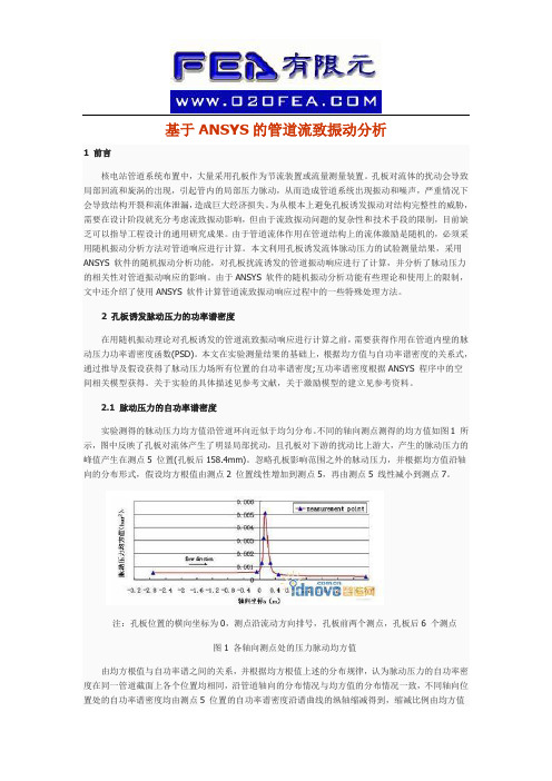
2.1 脉动压力的自功率谱密度实验测得的脉动压力均方值沿管道环向近似于均匀分布。
不同的轴向测点测得的均方值如图1 所示,图中反映了孔板对流体产生了明显局部扰动,且孔板对下游的扰动比上游大,产生的脉动压力的峰值产生在测点5 位置(孔板后158.4mm)。
忽略孔板影响范围之外的脉动压力,并根据均方值沿轴向的分布形式,假设均方根值由测点2 位置线性增加到测点5,再由测点5 线性减小到测点7。
注:孔板位置的横向坐标为0,测点沿流动方向排号,孔板前两个测点,孔板后6 个测点图1 各轴向测点处的压力脉动均方值由均方根值与自功率谱之间的关系,并根据均方根值上述的分布规律,认为脉动压力的自功率密度在同一管道截面上各个位置均相同,沿管道轴向的分布情况与均方值的分布情况一致,不同轴向位置处的自功率谱密度均由测点5 位置的自功率谱密度沿谱曲线的纵轴缩减得到,缩减比例由均方值沿管道的轴向分布确定。
ansys fluent中文版流体计算工程案例详解
ansys fluent中文版流体计算工程案例详解ANSYS Fluent是一种流体计算动力学软件,可用于解决各种流体力学问题。
本文将详细介绍ANSYS Fluent中文版的流体计算工程案例,包括案例的基本背景、模拟过程和结果分析。
这些案例旨在帮助用户深入了解ANSYS Fluent的使用方法和流体计算工程实践。
一个典型的案例是流体在管道中的流动。
该案例背景是,一根长直管道内有水流动,管道的直径为0.1米,长度为10米。
水的初始速度为1 m/s,管道的壁面是光滑的,管道两端的压差为100Pa。
现在需要使用ANSYS Fluent模拟该流体流动过程,并进一步分析不同参数对流动的影响。
首先,在ANSYS Fluent中创建一个新的仿真项目,并选择“仿真”模块。
在界面上点击“新建”按钮,在弹出的对话框中填写相应的参数,例如案例名称、计算器类型和尺寸单位。
点击“确定”后,进入模拟设置页面。
首先,需要定义获得流动场稳定解所需的物理模型和求解方法。
在“物理模型”选项卡中,选择“连续相”和“非恒定模型”。
在“湍流模型”中选择某种适合的模型,例如k-ε模型。
在“重力”选项卡中,定义流体的密度和重力加速度。
接下来,在“模型”选项卡中,定义管道的几何和边界条件。
选择“管道”作为流体领域的几何模型,并定义长度、直径和内壁面的润滑系数。
在“边界”选项卡中,定义管道两端的入口和出口条件,例如速度和压力。
将管道两端的压力差设置为100Pa,在入口处设置水的初始速度为1 m/s。
在出口处选择“出流”边界条件。
完成几何和边界条件的定义后,点击“模拟”选项卡进入模拟设置界面。
在“求解控制”中,设置计算时间步长和迭代次数。
选择合适的网格划分方法,并进行网格划分。
点击“网格”选项卡,选择合适的网格类型,并进行网格划分。
在划分网格后,可以使用“导入”按钮导入网格文件,并进行网格优化。
完成设置后,点击“计算”按钮开始进行模拟计算。
在计算过程中,可以实时观察流体场的变化情况,并通过Fluent Post-processing工具进行结果分析。
基于ANSYS的腐蚀压力管道的应力分析
1 e d rn e d n n t s r c s a d c ro in d ma e n e rt a a i i p o i e re e t e c n r1 i u g w l i g a d s e s c a k o rso a g ,a d a t oe il b s s rv d d f f ci o t . n i r n h c s o v o
芒
中现象加 剧 , 易发 生破坏 。 更
参考 文献 :
[] 蒋 1 奇, 隋青美 , 高 瑞. 管道缺 陷漏磁场和缺 陷尺寸关 系的研
究[ ] 无损检测 ,05,7 8 :9 - 9 . J. 20 2 ( )3 6 3 8
图 8 管 道应 力与腐蚀深度对应关系 曲线 图
[ ] 张喜艳 , 2 谭跃刚. 管道缺陷漏 磁检测信号 的仿 真[ ] 机械 ,0 8 J. 2 0
( )有 限元 计 算 结果 有 限元 计 算 结 果 如 表 1 2
和 图 2所示 。
道 内壁产 生均 匀腐 蚀 或 沿 轴 向产 生 沟槽 。因此 几 何 模 型 可简 化 为平 面应 变 问题 , 文 采 用平 面 板 单 元 本 pae2进 行模 拟分 析 J l 4 n 。无裂 缝模 型和 网格 划 分如
石 油 工程 建设 ,0 5,1 3 :7 1. 20 3 () 1—9
ansys经典算例:稳态管道流体分析
ansys经典算例:稳态管道流体分析Fluid #2: Velocity analysis of fluid flow in a channel USING FLOTRAN Introduction:In this example you will model fluid flow in a channelPhysical Problem:Compute and plot the velocity distribution within the elbow. Assume that the flow is uniform at both the inlet and the outlet sections and that the elbow has uniform depth.Problem Description:The channel has dimensions as shown in the figureThe flow velocity as the inlet is 10 cm/sUse the continuity equation to compute the flow velocity at exitObjective:To plot the velocity profile in the channelTo plot the velocity profile across the elbowYou are required to hand in print outs for the aboveFigure:IMPORTANT: Convert all dimensions and forces into SI unitsSTARTING ANSYSC lick on ANSYS 6.1in the programs menu.S elect Interactive.T he following menu comes up. Enter the working directory. All your files will be stored in this directory. Also under UseDefault Memory Model make sure the values 64 for Total Workspace, and 32 for Database are entered. To change these values unclick Use Default Memory ModelMODELING THE STRUCTUREG o to the ANSYS Utility Menu (the top bar)Click Workplane>WP Settings…The following window comes up:o Check the Cartesian and Grid Only buttonso Enter the values shown in the figure above•Go to the ANSYS Main Menu (on the left hand side of the screen) and click Preprocessor>Modeling>Create>Keypoints>On Working PlaneCreate keypoints corresponding to the vertices in the figure. The keypoints look like below.Now create lines joining these key points.M odeling>Create>Lines>Lines>Straight lineT he model looks like the one below.Now create fillets between lines L4-L5 and L1-L2.C lick Modeling>Create>Lines>Line Fillet. A pop-up window will now appear. Select lines 4 and 5. ClickOK. The following window will appear:This window assigns the fillet radius. Set this value to 0.1 m.Repeat this process of filleting for Lines 1 and 2.The model should look like this now:N ow make an area enclosed by these lines.M odeling>Create>Areas>Arbitrary>By LinesS elect all the lines and click OK. The model looks like the followingThe modeling of the problem is done.ELEMENT PROPERTIESSELECTING ELEMENT TYPE:•Click Preprocessor>Element Type>Add/Edit/Delete... In the 'Element Types' window that opens click on Add... The following window opens.•Type 1 in the Element type reference number.•Click on Flotran CFD and select 2D Flotran 141. Click OK. Close the Element types window.•So now we have selected Element type 1 to be solved using Flotran, the computational fluid dynamics portion of ANSYS. This finishes the selection of element type.DEFINE THE FLUID PROPERTIES:•Go to Preprocessor>Flotran Set Up>Fluid Properties.•On the box, shown below, set the first two input fields as Air-SI, and then click on OK. Another box will appear. Accept the default values by clicking OK.•Now we’re ready to define the Material PropertiesMATERIAL PROPERTIESWe will model the fluid flow problem as a thermal conduction problem. The flow corresponds to heat flux, pressure corresponds to temperature difference and permeability corresponds to conductance.Go to the ANSYS Main MenuClick Preprocessor>Material Props>Material Models. The following window will appearAs displayed, choose CFD>Density. The following window appears.Fill in 1.23 to set the density of Air. Click OK.Now choose CFD>Viscosity. The following window appears:Now the Material 1 has the properties defined in the above table so the Material Models window may be closed. MESHING: DIVIDING THE CHANNEL INTO ELEMENTS:G o to Preprocessor>Meshing>Size Cntrls>ManualSize>Lines>All Lines.I n the window that comes up type 0.01 in the field for 'Element edge length'.Now Click OK.Now go to Preprocessor>Meshing>Mesh>Areas>Free. Click the area and the OK. The mesh will look like thefollowing.BOUNDARY CONDITIONS AND CONSTRAINTSGo to Preprocessor>Loads>Define Loads>Apply>Fluid CFD>Velocity>On lines. Pick the left edge of the outer block and Click OK. The following window comes up.E nter 0.1 in the VX value field and click OK. The 0.1 corresponds to the velocity of 0.1 meter per second of air flowingfrom the left side.R epeat the above and set the Velocity to ZERO for the air along all of the edges of the pipe. (VX=VY=0 for all sides)O nce they have been applied, the pipe will look like this:•Go to Main Menu>Preprocessor>Loads>Define Loads>Apply>Fluid CFD>Pressure DOF>On Lines.•Pick the outlet line. (The horizontal line at the top of the area) Click OK.•Enter 0 for the Pressure value.•Now the Modeling of the problem is done.SOLUTIONG o to ANSYS Main Menu>Solution>Flotran Set Up>Execution Ctrl.•The following window appears. Change the first input field value to 300, as shown. No other changes are needed. Click OK.G o to Solution>Run FLOTRAN.W ait for ANSYS to solve the problem.C lick on OK and close the 'Information' window.POST-PROCESSINGPlotting the velocity distribution…Go to General Postproc>Read Results>Last Set.Then go to General Postproc>Plot Results>Contour Plot>Nodal Solution. The following window appears:•Select DOF Solution and Velocity VSUM and Click OK.•This is what the solution should look like:•Next, go to Main Menu>General Postproc>Plot Results>Vector Plot>Predefined.The following window will appear:•Select OK to accept the defaults. This will display the vector plot to compare to the solution of the same tutorial solved using the Heat Flux analogy. Note: This analysis is FAR more precise as shown by the followingsolution:•Go to Main Menu>General Postproc>Path Operations>Define Path>By Nodes•Pick points at the ends of the elbow as shown. We will graph the velocity distribution along the line joiningthese two points.•The following window comes up.•Enter the values as shown.•Now go to Main Menu>General Postproc>Path Operations>Map onto Path. The following window comes up.•Now go to Main Menu>General Postproc>Path Operations>Plot Path Items>On Graph.•The following window comes up.•Select VELOCITY and click OK.•The graph will look as follows:。
基于ANSYS的腐蚀管道的有限元分析

基于ANSYS的腐蚀管道的有限元分析摘要:本文应用有限元软件ANSYS对腐蚀管道进行承压分析,并分别仿真了腐蚀缺陷处的弹性失效、塑性失效和爆破失效压力,分析了腐蚀深度对三种失效模式的影响。
关键词:有限元软件ANSYS 服饰管道分析管道运输具有耗能少、成本低、效益好等优点。
随着管道服役年限的增长,油气管道会发生腐蚀穿孔给企业造成巨大的损失。
本文以含腐蚀缺陷的管道为研究对象,借助有限元软件ANSYS对管道在内压下弹塑性变形进行模拟,分析了腐蚀程度对管道承载能力的影响,对于及时采取降压、补强等技术措施,确保管道安全运行具有指导意义。
1 有限元模型1.1 失效准则由屈服准则实验结果的验证实验表明,一般韧性金属材料与von Mises准则符合较好,也就是说多数金属符合von Mises准则。
因此在本文的研究与分析中,采用von Mises塑性失效准则。
计算公式为:1.2 假定条件根据管线的特点,为了方便计算,进行了如下假定。
(1)管线材料具有塑性应力-应变状态。
(2)只考虑内压对管壁的作用。
(3)材料在屈服以后的硬化模量是常数。
1.3 模型机构和边界条件本文采用常见的管道腐蚀类型沟槽状腐蚀。
同时由于腐蚀缺陷破坏了管道的整体结构,不能采用壳单元。
由于实际管道很长,可以认为没有受到轴力的作用。
建模时采用三维实体结构,并使用solid185单元。
1.4 管体材料及性能参数1.5 腐蚀管段有限元模型2 仿真结果及分析内压从1 MPa开始,取步长为1 MPa,仿真完成后在通用后处理器中找出腐蚀处失效压力P,然后再取步长为0.1 MPa,在(P-1,P)区间内再次进行仿真计算,分别找出不同深度腐蚀的弹性失效压力、塑性失效压力和爆破失效压力。
结果如表2所示。
从仿真结果看,当腐蚀长度和宽度不变时,随着腐蚀深度的增加,管线的弹性失效、塑性失效和爆破失效压力明显降低。
失效压力与深度的尺寸关系表明,弹性失效压力由于有应力集中的影响,下降的比较快,而塑性失效压力和爆破失效压力则比较稳定,结果如表(图3)所示。
ansys工程实例(4经典例子)
输气管道受力分析(ANSYS建模)任务和要求:按照输气管道的尺寸及载荷情况,要求在ANSYS中建模,完成整个静力学分析过程。
求出管壁的静力场分布。
要求完成问题分析、求解步骤、程序代码、结果描述和总结五部分。
所给的参数如下:材料参数:弹性模量E=200Gpa; 泊松比0.26;外径R₁=0.6m;内径R₂=0.4m;壁厚t=0.2m。
输气管体内表面的最大冲击载荷P为1Mpa。
四.问题求解(一).问题分析由于管道沿长度方向的尺寸远大于管道的直径,在计算过程中忽略管道的端面效应,认为在其长度方向无应变产生,即可将该问题简化为平面应变问题,选取管道横截面建立几何模型进行求解。
(二).求解步骤定义工作文件名选择Utility Menu→File→Chang Jobname 出现Change Jobname对话框,在[/FILNAM] Enter new jobname 输入栏中输入工作名LEILIN10074723,并将N ew log and eror file 设置为YES,单击[OK]按钮关闭对话框定义单元类型1)选择Main Meun→Preprocessor→Element T ype→Add/Edit/Delte命令,出现Element T ype 对话框,单击[Add]按钮,出现Library of Element types对话框。
2)在Library of Element types复选框选择S trctural、Solid、Quad 8node 82,在Element type reference number输入栏中出入1,单击[OK]按钮关闭该对话框。
3. 定义材料性能参数1)单击Main Meun→Preprocessor→Material Props→Material models出现Define Material Behavion 对话框。
选择依次选择S tructural、Linear、Elastic、Isotropic选项,出现Linear Isotropic Material Properties For Material Number 1对话框。
ANSYS-APDL命令流分析蒸汽管道
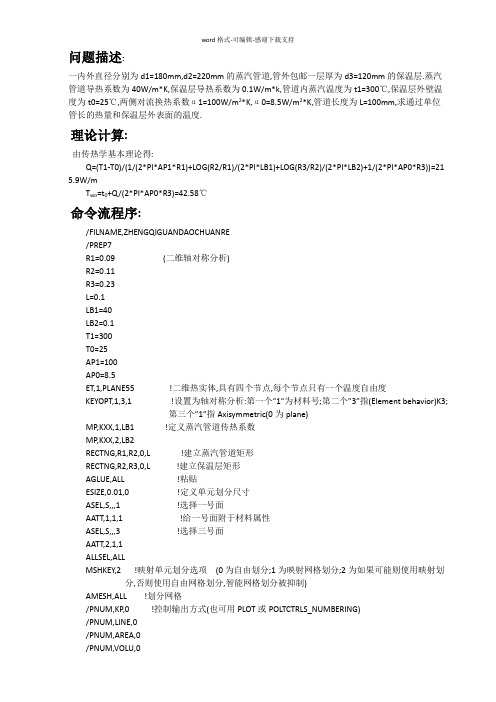
问题描述:一内外直径分别为d1=180mm,d2=220mm的蒸汽管道,管外包邮一层厚为d3=120mm的保温层.蒸汽管道导热系数为40W/m*K,保温层导热系数为0.1W/m*k,管道内蒸汽温度为t1=300℃,保温层外壁温度为t0=25℃,两侧对流换热系数α1=100W/m2*K,α0=8.5W/m2*K,管道长度为L=100mm,求通过单位管长的热量和保温层外表面的温度.理论计算:由传热学基本理论得:Q=(T1-T0)/(1/(2*PI*AP1*R1)+LOG(R2/R1)/(2*PI*LB1)+LOG(R3/R2)/(2*PI*LB2)+1/(2*PI*AP0*R3))=21 5.9W/mT wo=t0+Q/(2*PI*AP0*R3)=42.58℃命令流程序:/FILNAME,ZHENGQIGUANDAOCHUANRE/PREP7R1=0.09 (二维轴对称分析)R2=0.11R3=0.23L=0.1LB1=40LB2=0.1T1=300T0=25AP1=100AP0=8.5ET,1,PLANE55 !二维热实体,具有四个节点,每个节点只有一个温度自由度KEYOPT,1,3,1 !设置为轴对称分析:第一个”1”为材料号;第二个”3”指(Element behavior)K3;第三个”1”指Axisymmetric(0为plane)MP,KXX,1,LB1 !定义蒸汽管道传热系数MP,KXX,2,LB2RECTNG,R1,R2,0,L !建立蒸汽管道矩形RECTNG,R2,R3,0,L !建立保温层矩形AGLUE,ALL !粘贴ESIZE,0.01,0 !定义单元划分尺寸ASEL,S,,,1 !选择一号面AATT,1,1,1 !给一号面附于材料属性ASEL,S,,,3 !选择三号面AATT,2,1,1ALLSEL,ALLMSHKEY,2 !映射单元划分选项(0为自由划分;1为映射网格划分;2为如果可能则使用映射划分,否则使用自由网格划分,智能网格划分被抑制)AMESH,ALL !划分网格/PNUM,KP,0 !控制输出方式(也可用PLOT或POLTCTRLS_NUMBERING)/PNUM,LINE,0/PNUM,AREA,0/PNUM,VOLU,0/PNUM,NODE,1/PNUM,TABN,0/PNUM,SVAL,0/NUMBER,1/PNUM,MAT,1SFL,4,CONV,AP1,,T1 !在四号面上施加对流换热载荷,AP1为膜系数SFL,6,CONV,AP0,,T0FINISH/SOLUANTYPE,STATICTIME,1 !定义求解时间SOLVEFINISH/POST1 !进入后处理器SET,LAST !读入最后子步结果FLST,2,15,1 !”2”为第二个参数;”15”为路径上有15个节点;”1”为节点编号FITEM,2,1 !用POLTCTRLS_NUMBERING显示Y=0的节点,依次拾取FITEM,2,3FITEM,2,2FITEM,2,35FITEM,2,36FITEM,2,37FITEM,2,38FITEM,2,39FITEM,2,40FITEM,2,41FITEM,2,42FITEM,2,43FITEM,2,44FITEM,2,45FITEM,2,34PATH,RR2,23,30,20 !建立径向路径PPATH,P51X,1PATH,STATPDEF,TRR,TEMP,,AVG !向路径上映射温度分析结果PLPATH,TRR !显示路径温度变化曲线图PLPAGM,TRR,1,BLANK !显示径向温度分布云图(二维)PLNSOL,TEMP,,0 !显示径向温度分布云图(三维)/EXPAND,27,AXIS,,,10 !扩展至3/4圆柱体:”10”为每10度为单位,”27”为27*10=270度即3/4圆柱;AIXS是关于Y轴做如上旋转扩展PLNSOL,TEMP,,0 !显示维度分布云图/EXPAND*GET,TWO,NODE,34,TEMP !获取蒸汽管道外壁34号节点的温度NSEL,S,LOC,X,R1 !选择所有X坐标为R1的节点,即管道内表面ESLN !选择依附于上条命令所选节点的单元ETABLE,HT1,HEAT !生成一个单元表SSUM !计算热损失*GET,HT,SSUM,,ITEM,HT1 !获取热参数PI=3.1415926 !理论计算QF=(HT)/LLQ=(T1-T0)/(1/(2*PI*AP1*R1)+LOG(R2/R1)/(2*PI*LB1)+LOG(R3/R2)/(2*PI*LB2)+1/(2*PI*AP0*R3)) LTWO=T0+LQ/(2*PI*AP0*R3)TER=1-LTWO/TWOQER=1-LQ/QF*STATUS,PARM !列出所有参数PARAMETER STATUS- ( 44 PARAMETERS DEFINED)(INCLUDING 26 INTERNAL PARAMETERS)NAME VALUE TYPE DIMENSIONS AP0 8.50000000 SCALARAP1 100.000000 SCALARHT 21.5958285 SCALARL 0.100000000 SCALARLB1 40.0000000 SCALARLB2 0.100000000 SCALARLQ 215.886634 SCALARLTWO 42.5751537 SCALARPI 3.14159260 SCALARQER 3.317851283E-04 SCALARQF 215.958285 SCALARR1 9.000000000E-02 SCALARR2 0.110000000 SCALARR3 0.230000000 SCALART0 25.0000000 SCALART1 300.000000 SCALARTER 1.369849885E-04 SCALARTWO 42.5809866 SCALAR。
输气管道受力分析的ANSYS实现

现代CAE 技术及应用(ANSY)S输气管道受力分析的ANSYS实现一、问题描述一天然气输送管道的横截面及受力简图如图所示,在其内表面承受气体压力P的作用,求管壁的应力场分布。
图i管道受力简图管道几何参数:外径 R1=0.6m ;内径R2=0.4m ;壁厚t=0.2m。
管道材料参数:弹性模量E=200Gpa ;泊松比v =0.26。
载荷:P=1Mpa。
二、问题分析由于管道沿长度方向的尺寸远大于管道的直径,在计算过程中忽略管道的端面效应,认为在其长度方向无应变产生,即可将该问题简化为平面应变问题,选取管道横截面建立几何模型进行求解。
三、求解步骤1.定义单元类型定义单元类型为 Structural Solid , Quad 8node 82。
设置选项为 Plane strain。
图2定义单元类型WP 丼 0UP ¥tlRnadi-lThe<d-1 t) Rad-2 eTfiTht-td-2OKno setGance 1Help图4生产部分圆环面 图5生产的几何模型结果显示2. 定义材料性能参数 输入弹性模量和泊松比。
3. 生成几何模型,划分网格在ANSYS 窗口创建几何模型,如图 格,如图6所示。
然后保存。
4。
转换成圆柱坐标系后划分网图3定义材料性能参数Pic ]<UnvlclfWP X图6划分网格结果显示4、加载求解1)选择分析类型为 Static,对线段2和9施加X方向的位移约束,对线段4和7施加Y方向的位移约束。
对管道内环面施加压力。
图7选择分析类型图8施加位移约束对话框图9施加位移约束、压力之后的模型保存之后求解,出现图所示的提示。
图10求解结果提示5、查看求解结果查看受力前与受力后的形状变化。
图11受力后形状变化显示位移场等值线图。
iroAi HTiirTrnrTTET-l 列0 -1rfiSJTi (17G ]R5TS-CI1|^E-OS 血-,445T-05 Mt SKlt-Li^i.5LEE-O5■汕加■鹉■加迹“%■讯g■広flTX 茹EDU11] D2HI.4J3E-O5 .4TJE-O54妣5.4= IE -r5.53&E-O5■■rSTliATTIFTT.SB -1TIHE^lHHZ 5E0T-口£STM Z6 2D11.Ill DI102AN显示X 方向应力等值线图。
- 1、下载文档前请自行甄别文档内容的完整性,平台不提供额外的编辑、内容补充、找答案等附加服务。
- 2、"仅部分预览"的文档,不可在线预览部分如存在完整性等问题,可反馈申请退款(可完整预览的文档不适用该条件!)。
- 3、如文档侵犯您的权益,请联系客服反馈,我们会尽快为您处理(人工客服工作时间:9:00-18:30)。
Modeling and Meshing Guide | Chapter 10. Piping Models |
10.3. Sample Input
Consider the following sample piping data input:
! Sample piping data input
!
/FILNAM,SAMPLE
/TITLE, SAMPLE PIPING INPUT
/UNITS,BIN ! A reminder that consistent units are U. S. Customary inches
!
/PREP7
! Define material properties for pipe elements
MP,EX,1,30e6
MP,PRXY,1,0.3
MP,ALPX,1,8e-6 !thermal expansion coefficient 热膨胀系数
MP,DENS,1,.283
PUNIT,1 ! Units will be read as ft+in+fraction and converted to
! decimal inches
PSPEC,1,8,STD ! 8" standard pipe
POPT,B31.1 ! Piping analysis standard: ANSI B31.1
PTEMP,200 ! Temperature = 200°
PPRES,1000 ! Internal pressure = 1000 psi
PDRAG,,,-.2 ! Drag = 0.2 psi in -Z direction at any height (Y) BRANCH,1,0+12,0+12 ! Start first pipe run at (12",12",0")
RUN,,7+4 ! Run 7'-4" in +Y direction
RUN,9+5+1/2 ! Run 9'-5 1/2" in +X direction
RUN,,,-8+4 ! Run 8'-4" in -Z direction
RUN,,8+4 ! Run 8'-4" in +Y direction
/PNUM,NODE,1 !图示节点及编号
/VIEW,1,1,2,3
EPLOT ! Identify node number at which 2nd run starts BRANCH,4 ! Start second pipe run at node 4
RUN,6+2+1/2 ! Run 6'-2 1/2" in +X direction
TEE,4,WT ! Insert a tee at node 4 T形管
/PNUM,DEFA 恢复编号为默认值
/PNUM,ELEM,1
EPLOT ! Identify element numbers for bend and miter inserts BEND,1,2,SR ! Insert a "short-radius" bend between elements 1 and 2
MITER,2,3,LR,2 ! Insert a two-piece miter between elements 2 and 3
/PNUM,DEFA
/PNUM,NODE,1
! Zoom in on miter bend to identify nodes for spring hangers
/ZOOM, 1, 242.93 , 206.62 , -39.059 , 26.866 PSPRNG,14,TRAN,1e4,,0+12 ! Insert Y-direction spring at node 14 PSPRNG,16,TRAN,1e4,,0+12 ! Insert Y-direction spring at node 16 ! List and display interpreted input data
/AUTO
/PNUM,DEFA
EPLOT
NLIST
ELIST
SFELIST !面载荷surface loads
BFELIST !体载荷body
See the descriptions of the PUNIT, /PSPEC, POPT, PTEMP, PPRES, PDRAG, BRANCH, TEE, /PNUM, MITER, /ZOOM, PSPRNG, /AUTO, SFELIST, and BFELIST commands in the Commands Reference for more information.
Note
While two hangers are provided, more restraints are needed before proceeding to solution.
Figure 10.1 Sample Piping Input
PUNIT,1
Main Menu> Preprocessor> Modeling> Create> Piping Models>
Specifications 说明
10.2. Modeling Piping Systems with Piping Commands。