2006s4f
PETS2006年基准数据-数据集S4 (Take 5-A)(PETS 2006 Benchmark Data-Dataset S4 (Take 5-A))
PETS2006年基准数据-数据集S4 (Take 5-A)(PETS 2006 Benchmark Data-Dataset S4 (Take 5-A))数据介绍:The data-sets are multi-sensor sequences containing left-luggage scenarios with increasing scene complexity. The results of processing the datasets are to submitted in XML format (details below).关键词:PETS 2006年,基准,被留下的行李,多传感器序列,情景, PETS 2006,benchmark,Left-Luggage,multi-sensor sequences,scenarios,数据格式:IMAGE数据详细介绍:PETS 2006 Benchmark Data- DatasetOverviewThe data-sets are multi-sensor sequences containing left-luggage scenarios with increasing scene complexity. The results of processing the datasets are to submitted in XML format (details below).Please e-mail datasets@ if you require assistance obtaining these data-sets for the workshop.Aims and ObjectivesThe aim of this workshop is to use existing systems for the detection of left (i.e. abandoned) luggage in a real-world environment. The scenarios are filmed from multiple cameras and involve multiple actors.Definition of Left-LuggageLeft-luggage in the context of PETS 2006 is defined as items of luggage that have been abandoned by their owner. In the published scenarios each item of luggage has one owner and each person owns at most one item of luggage.To implement a system based on this definition there are three additional components that need to be defined:A.What items are classed as luggage? Luggage is defined to include all types of baggage that can be carried by hand e.g. trunks, bags, rucksacks, backpacks, parcels, and suitcases.Five common types of luggage are considered in this study:1.Briefcase2.Suitcase3.25 litre rucksack4.70 litre backpack5.Ski gear carrierB.What constitutes attended and unattended luggage? In this study three rules are used to determine whether luggage is attended to by a person (or not):1. A luggage is owned and attended to by a person who enters the scenewith the luggage until such point that the luggage is not in physicalcontact with the person (contextual rule).2.At this point the luggage is attended to by the owner ONLY when theyare within a distance a metres of the luggage (spatial rule). All distances are measured between object centroids on the ground plane (i.e. z=0).The image below shows a person within a (=2) metres of their luggage.In this situation no alarm should be raised by the system.3. A luggage item is unattended when the owner is further than b metres(where b>=a *) from the luggage. The image below shows a personcrossing the line at b (=3) metres. In this situation the system shoulduse the spatio-temporal rule in item C, below, to detect whether thisitem of luggage has been abandoned (an alarm event).* If b > a, the distance between radii a and b is determined to be a warning zone where the luggage is neither attended to nor left unattended. This zone is defined to separate the detection points of the two states, reducing uncertainties introduced due to calibration / detection errors in the sensorsystem etc. The image below shows a person crossing the line at a (=2) metres, but within the radius b (=3) metres. In this scenario the system can be set up to trigger a warning event, using a rule similar to the spatio-temporal rule in item C, below. Both warning and alarm events will be given in the ground truth.C. What constitutes abandonment of luggage by the owner? The abandonment of an item of luggage is defined spatially and temporally. Abandonment (causing an alarm) is defined as:1.An item of luggage that has been left unattended by the owner for aperiod of t consecutive seconds in which time the owner has notre-attended to the luggage, nor has the luggage been attended to by a second party (instigated by physical contact, in which case a theft /tampering event may be raised). The image below shows an item ofluggage left unattended for t (=30) seconds, at which point the alarmevent is triggered.Calibration DataThe geometric patterns on the floor of the station were used for calibration purposes. The following point locations were used as the calibration pattern (click to view full 1800x500 resolution image):All spatial measurements are in metres. The provided calibration parameters were obtained using the freely available Tsai Camera Calibration Software by Reg Willson. For instructions on how to use Reg Willsons software visit Chris Needhams helpful page. More information on the Tsai camera model is available on CVonline.An example of the provided calibration parameter XML file is given here. This XML file contains Tsai camera parameters obtained from Reg Willsons software (output file), using this reference image and this set of points. C++ code (available here) is provided to allow you to load and use the calibration parameters in your program (courtesy of project ETISEO).The DV cameras used to film all data-sets are:Camera 1: Canon MV-1 1xCCD w/progressive scanCamera 2: Sony DCR-PC1000E 3xCMOSCamera 3: Canon MV-1 1xCCD w/progressive scanCamera 4: Sony DCR-PC1000E 3xCMOSThe resolution of all sequences are PAL standard (768 x 576 pixels, 25 frames per second) and compressed as JPEG image sequences(approx. 90% quality).XML schemaAll scenarios come with two XML files. The first of these files contains camera calibration parameters, these are given in the sub-directory 'calibration'. See the previous section (Calibration Data) for information on this XML file format.The second XML file (given in the sub-directory 'xml') contains both configuration and ground-truth information. This xml format is also used for submission of results.The XML schema for the configuration / ground-truth / submission is given here.The XML files provided contain scenario details, parameters and ground-truth information (e.g. the radii distances, luggage location, warning / alarm triggers etc). A fully commented example of the provided XML is given here.For submitted XML not all details need to be provided. An example of the (minimum) data to be submitted is given here.Dataset S1 (Take 1-C)Scenario: left luggageElements: 1 person, 1 luggage itemGround truth parameters: a = 2 metres, b = 3 metres, t = 30 secondsSubjective Difficulty:This scenario contains a single person with a rucksack who loiters before leaving the item of luggage unattended.Sample ImagesThe following images show representative images captured from cameras 1-4.DownloadThe entire scenario including the calibration and ground truth data S1-T1-C.zip, (1.10Gb)Dataset S2 (Take 3-C)Scenario: left luggageElements: 2 people, 1 luggage itemGround truth parameters: a = 2 metres, b = 3 metres, t = 30 secondsSubjective Difficulty:This scenario contains two people who enter the scene from opposite directions. One person places a suitcase on the ground, before both people leave together (without the suitcase).Sample ImagesThe following images show representative images captured from cameras 1-4.DownloadThe entire scenario including the calibration and ground truth data S2-T3-C.zip, (0.93Gb)Dataset S3 (Take 7-A)Scenario: left luggageElements: 1 person, 1 luggage itemGround truth parameters: a = 2 metres, b = 3 metres, t = 30 secondsSubjective Difficulty:This scenario contains a person waiting for a train, the person temporarily places their briefcase on the ground before picking it up again and moving to a nearby shop.Sample ImagesThe following images show representative images captured from cameras 1-4.DownloadThe entire scenario including the calibration and ground truth data S3-T7-A.zip, (0.88Gb)Dataset S4 (Take 5-A)Scenario: left luggageElements: 2 people, 1 luggage itemGround truth parameters: a = 2 metres, b = 3 metres, t = 30 secondsSubjective Difficulty:This scenario contains a person placing a suitcase on the ground. Following this a second person arrives and talks with the first person. The first person leaves the scene without their luggage. Distracted by a newspaper, the second person does not notice that the first persons luggage is left unattended.Sample ImagesThe following images show representative images captured from cameras 1-4.DownloadThe entire scenario including the calibration and ground truth data S4-T5-A.zip, (1.04Gb)Dataset S5 (Take 1-G)Scenario: left luggageElements: 1 person, 1 luggage itemGround truth parameters: a = 2 metres, b = 3 metres, t = 30 secondsSubjective Difficulty:This scenario contains a single person with ski equipment who loiters before abandoning the item of luggage.Sample ImagesThe following images show representative images captured from cameras 1-4.DownloadThe entire scenario including the calibration and ground truth data S5-T1-G.zip, (1.25Gb)Dataset S6 (Take 3-H)Scenario: left luggageElements: 2 people, 1 luggage itemGround truth parameters: a = 2 metres, b = 3 metres, t = 30 secondsSubjective Difficulty:This scenario contains two people who enter the scene together. One person places a rucksack on the ground, before both people leave together (without the rucksack).Sample ImagesThe following images show representative images captured from cameras 1-4.DownloadThe entire scenario including the calibration and ground truth data S6-T3-H.zip, (0.98Gb)Dataset S7 (Take 6-B)Scenario: left luggageElements: 6 people, 1 luggage itemGround truth parameters: a = 2 metres, b = 3 metres, t = 30 secondsSubjective Difficulty:This scenario contains a single person with a suitcase who loiters before leaving the item of luggage unattended. During this event five other people move in close proximity to the item of luggage.Sample ImagesThe following images show representative images captured from cameras 1-4.DownloadThe entire scenario including the calibration and ground truth data S7-T6-B.zip, (1.22Gb)Additional InformationThe scenarios can also be downloaded fromftp:///pub/PETS2006/ (use anonymous login). Warning:ftp:// is not listing files correctly on some ftp clients. If you experience problems you can connect to the http server at/PETS2006/.Legal note: The UK Information Commisioner has agreed that the PETS 2006 data-sets described here may be made publicly available for the purposes of academic research. The video sequences are copyright ISCAPS consortium and permission is hereby granted for free download for the purposes of the PETS 2006 workshop.数据预览:点此下载完整数据集。
深圳南瑞IEC103例子报文
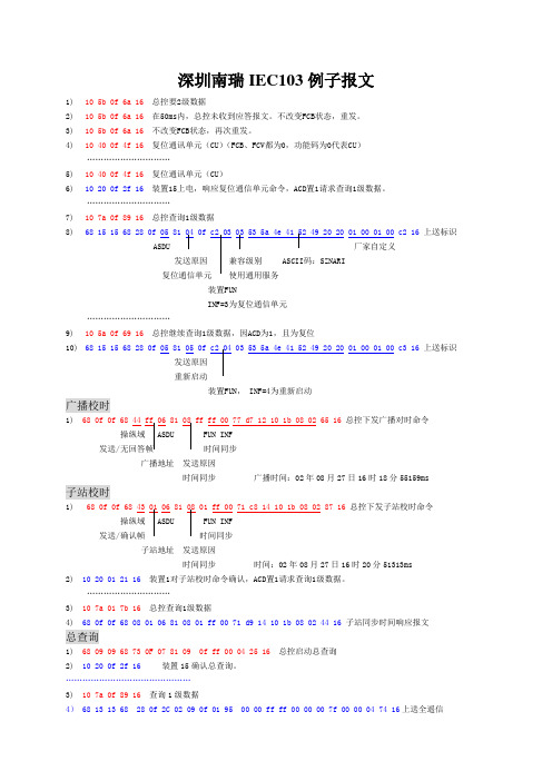
深圳南瑞IEC103例子报文1)10 5b 0f 6a 16总控要2级数据2)10 5b 0f 6a 16 在50ms内,总控未收到应答报文。
不改变FCB状态,重发。
3)10 5b 0f 6a 16不改变FCB状态,再次重发。
4)10 40 0f 4f 16复位通讯单元(CU)(FCB、FCV都为0,功能码为0代表CU)…………………………5)10 40 0f 4f 16复位通讯单元(CU)6)10 20 0f 2f 16装置15上电,响应复位通信单元命令,ACD置1请求查询1级数据。
…………………………7)10 7a 0f 89 16总控查询1级数据8)68 15 15 68 28 0f 05 81 04 0f c2 03 03 53 5a 4e 41 52 49 20 20 01 00 01 00 c2 16上送标识厂家自定义发送原因ASCII码:SZNARI装置FUNINF=3为复位通信单元…………………………9)10 5a 0f 69 16总控继续查询1级数据,因ACD为1,且为复位10)68 15 15 68 28 0f 05 81 05 0f c2 04 03 53 5a 4e 41 52 49 20 20 01 00 01 00 c3 16上送标识发送原因重新启动装置FUN, INF=4为重新启动广播校时1) 68 0f 0f 68 44 ff 06 81 08 ff ff 00 77 d7 12 10 1b 08 02 65 16 总控下发广播对时命令发送/时间同步广播地址发送原因时间同步广播时间:02年08月27日16时18分55159ms子站校时1) 68 0f 0f 68 43 01 06 81 08 01 ff 00 71 c8 14 10 1b 08 02 87 16 总控下发子站校时命令操纵域发送/确认帧时间同步子站地址发送原因时间同步时间:02年08月27日16时20分51313ms2) 10 20 01 21 16装置1对子站校时命令确认,ACD置1请求查询1级数据。
我国电离层闪烁初步观测结果
第19卷增刊2004年10月电波科学学报CHINESEJOURNALOFRADIOSCIENCEV01.19,Sup.October,2004我国电离层闪烁初步观测结果陈丽甄卫民马宝田(中国电波传播研究所青岛分所,chenli.qd@163.corncrirp—zwm@163.com,山东青岛266071)摘要电离层闪烁观测是研究电离层闪烁现象及其效应的实验基础。
本文中利用自行研制的电离层闪烁监测仪,开展了在我国中低纬地区的闪烁观测,初步的结果表明电离层闪烁在中低纬地区发生频繁,且对UHF频段通信卫星的影响十分严重。
关键词电离层闪烁,观更’通信影响1引言2电离层闪烁监测仪的简介电离层闪烁的效应之一是导致信号幅度的衰落,使信道的信噪比下降,误码率上升,严重时使卫星通信链路中断。
这种现象在低纬度地区的夜间尤为频繁,影响也最严重。
我国长江(上海、武汉、重庆)以南的低纬度地区,特别是台湾、福建、广东、广西、海南及南海地区都是电离层闪烁的高发区,对通信的影响也比较严重。
通过对UHF频段用户的调研得知,信号在夜间经常出现干扰(特别是在南方地区)甚至出现信号中断的现象。
进行电离层闪烁的观测是研究电离层闪烁现象及其效应的实验基础。
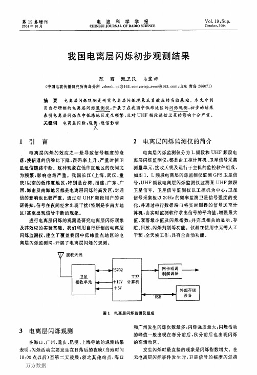
我们利用自行研制的电离层闪烁监测仪,建立了覆盖我国中低纬重点地区的电离层闪烁监测网,开展了电离层闪烁的观测。
电离层闪烁监测仪分为L频段和UHF频段电离层闪烁监测仪,都是由工控计算机、卫星信号采集测量单元、接收天线及运行于主机的监控软件组成,如图1。
L频段电离层闪烁监测仪监测GPS卫星信号,UHF频段电离层闪烁监测仪监测某UHF频段卫星信号。
卫星信号监测仪以工控机为中心,卫星信号采集板以20Hz的频率监测卫星信号强度的变化,并通过串行数据端口将实时测得的信号送至计算机,由实时监测软件求出信号的平均值、增强最大值、衰落最小值及闪烁指数,并完成相关的显示、存贮、回放、闪烁判别等功能。
仪器在使用中无需人工干预,全天候工作,具有全自动功能。
国外不锈钢牌号对照表

Z12CN17.07 SUS301 301
—
SUS301J1 —
Z10CN18.09 SUS302 302
S30100 30301 301S21 14
——
——
S30200 30302 302S25 12
— — 2331
Z10CNF18.09 SUS303 303 S30300 30303 303S21 17 2346
32 00Cr19Ni13Mo3 03X16H15M3 X2CrNiMo18.16
33 0Cr18Ni16Mo5 —
—
34 1Cr18Ni9Ti
12X18H9T X12CrNiTi18.9
35 0Cr18Ni10Ti
08X18H10T X10CrNiTi18.9
36 1Cr18Ni11Ti
12X18H10T —
中国 (GB)
前苏联 (TOCT)
德国 (DIN)
1 奥 1Cr17Mn6Ni5N 12X17T9AH4 —
2 1Cr18Mn8Ni5N 12X17T9AH4 X8CrMnNi189
3 1Cr18Mn10Ni5Mo3N —
—
4 2Cr13Mn9Ni4
5 氏 1Cr17Ni7 6 1Cr17Ni8 7 1Cr18Ni9
51 Y1Cr17
—
X12CrMoS17
52 型 1Cr17Mo
—
X6CrMo17
53 00Cr17Mo
—
—
54 钢 00Cr18Mo2
—
—
55 1Cr25Ti
15X25T
X8Cr28
56 00Cr27Mo
—
—
—
SUS317 317
高中化学竞赛初赛模拟试卷 (36)
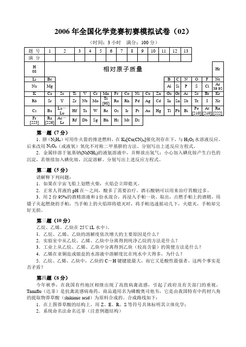
2006年全国化学竞赛初赛模拟试卷(02)(时间:3小时满分:100分)第一题(7分)1.肼(N2H4)可用作火箭的推进燃料,在K3[Cu(CN)4]催化剂存在下,与H2O2水溶液反应。
后来改用N2O4(或液氧)氧化不对称二甲基肼的方法。
分别写出上述反应方程式。
2.金属锌溶于氨基钠(NaNH2)的液氨溶液中,并释放出氢气;小心加入碘化铵产生白色的沉淀,若继续加入碘化铵,沉淀溶解。
分别写出上述反应方程式。
第二题(5分)请解释下列问题:1.如果在宇宙飞船上划燃火柴,火焰会立即熄灭。
2.正常人胃液的pH在~之间,酸多了需要治疗。
酒石酸钠可以用来治疗胃酸过多。
3.用2份95%的酒精溶液和l份水混合,再浸入手帕一块。
取出,点燃手帕上的酒精,用镊子夹起燃烧的手帕,当手帕上的火焰即将熄灭时,将手帕迅速摇动几下,火熄灭,手帕却完好无损。
第三题(10分)乙烷、乙烯、乙炔在25℃1L水中)。
1.乙烷、乙烯、乙炔的溶解度依次增大的主要原因是什么?2.实验室中从乙烷、乙烯、乙炔中分离得到纯净乙烷的方法是什么?3.工业上从乙烷、乙烯、乙炔中分离得到乙炔(较高含量)的简便方法是什么?4.乙烯在亚铜盐或银盐的水溶液中溶解度比在纯水中大得多,为什么?5.乙烷、乙烯、乙炔中,乙炔的C-H键键能最大,而它又是酸性最强者。
这两个事实是否矛盾?第四题(8分)今年秋季,在我国有些地区相继出现了高致病禽流感,引起了政府及有关部门的重视,Tamiflu(达菲)是抗禽流感病毒药,商品通用名为磷酸奥司他韦,它是由我国特有中药材八角的提取物莽草酸(shikimic acid)为原料合成的。
合成路线如下:1.在上图莽草酸的结构上,用Z、E、R、S等符号具体标明其立体化学;2.系统命名法命名达菲(注意例题结构)3.由莽草酸合成中间产物A 时需要添加哪2种原料,写出化学名称;4.由莽草酸合成达菲使用了10个步骤,除引入一些基团外,还有1个重要作用是什么?第五题(7分)1.在[Cr(NH 3)4Cl 2]+的光谱中是否存在金属-氯的振动红外光谱带,为什么?2.为了证明旋光性与分子中是否存在碳原子无关,Wemer 制备了[Co{(HO)2Co(NH 3)4}3]6+。
YZP(F)系列电机样本(最新版)
一、概述YZP 、YZPF 系列起重专用变频调速三相异步电动机是本公司总结变频调速三相异步电动机的成功经验而开发的起重机专用变频调速三相异步电动机。
充分吸改了近年来国内外变频调速方面的先进技术,特别适用于起重机高起动转矩和频繁起动的要求。
能与国内外各种变频装置配套,构成交流调速成系统,具有较高的精度和高的动态性能。
电动机基本技术要求符合IEC34-1和GB755国际和国家标准要求,安装尺寸符合IEC72国际标准。
二、型号说明异步电动机极数起重用铁芯长度代号变频调速机座长度代号强迫风冷中心高(㎜三、使用条件海拔小于1000M ,环境温度小于40℃,相对湿度小于90%,对不同环境温度及安装海拔高度按下表选取电机功率。
安装海拔高度(m环境温度1000 1500 2000 2500 300030℃ 100% 100% 100% 98% 95% 35℃ 100% 100% 97% 94% 91% 40℃ 100% 97% 93% 90% 87% 45℃ 95% 92% 88% 85% 83% 50℃ 90% 87% 84% 81% 55℃ 85% 82% 60℃ 80%四、电机的工作制、冷却方式、防护等级及安装型式1.YZP 系列电机的基准工作制为S3,负载持续率为40%;YZPF 系列电机的工作制为S3,负载持续率为60%。
不同工作制下功率折算表YZP 系列电机 S3 S3 6次/小时S4 S5 150次/小时 S4 S5 300次/小时 S4 S5 600次/小时工作制 30分钟 60分钟15% 25% 40% 60%100%25%40%60% 40% 60% 60%功率折算系数 1.0 1.0 1.0 1.0 1.0 0.85 0.72 1.0 0.85 0.75 0.72 0.64 0.50YZPF 系列电机 S3 S3 6次/小时 S4 S5 150次/小时 S4 S5 300次/小时 S4 S5600次/小时工作制30分钟60分钟15% 25% 40% 60%100%25%40%60%40% 60% 60% 功率折算系数1.0 1.0 1.0 1.0 1.0 1.00.9 1.0 1.0 0.850.80 0.70 0.602.YZP系列冷却方式为IC411(全封闭、自带风扇冷却;YZPF系列冷却方式为IC416(全封闭,轴向风冷却。
小学奥数几何五大模型之蝴蝶模型与相似模型

板块一 任意四边形模型任意四边形中的比例关系(“蝴蝶定理”):S 4S 3S 2S 1O DCBA①1243::S S S S =或者1324S S S S ⨯=⨯ ②()()1243::AO OC S S S S =++蝴蝶定理为我们提供了解决不规则四边形的面积问题的一个途径.通过构造模型,一方面可以使不规则四边形的面积关系与四边形内的三角形相联系;另一方面,也可以得到与面积对应的对角线的比例关系.【例 1】 (小数报竞赛活动试题)如图,某公园的外轮廓是四边形ABCD ,被对角线AC 、BD 分成四个部分,△AOB 面积为1平方千米,△BOC 面积为2平方千米,△COD 的面积为3平方千米,公园由陆地面积是6.92平方千米和人工湖组成,求人工湖的面积是多少平方千米?A【分析】 根据蝴蝶定理求得312 1.5AOD S =⨯÷=△平方千米,公园四边形ABCD 的面积是123 1.57.5+++=平方千米,所以人工湖的面积是7.5 6.920.58-=平方千米【巩固】如图,四边形被两条对角线分成4个三角形,其中三个三角形的面积已知,求:⑴三角形BGC 的面积;⑵:AG GC =?例题精讲任意四边形、梯形与相似模型B【解析】 ⑴根据蝴蝶定理,123BGCS ⨯=⨯,那么6BGCS=;⑵根据蝴蝶定理,()():12:361:3AG GC =++=. (???)【例 2】 四边形ABCD 的对角线AC 与BD 交于点O (如图所示).如果三角形ABD 的面积等于三角形BCD 的面积的13,且2AO =,3DO =,那么CO 的长度是DO 的长度的_________倍.AB C DOH GA BC D O【解析】 在本题中,四边形ABCD 为任意四边形,对于这种”不良四边形”,无外乎两种处理方法:⑴利用已知条件,向已有模型靠拢,从而快速解决;⑵通过画辅助线来改造不良四边形.看到题目中给出条件:1:3ABDBCDSS=,这可以向模型一蝴蝶定理靠拢,于是得出一种解法.又观察题目中给出的已知条件是面积的关系,转化为边的关系,可以得到第二种解法,但是第二种解法需要一个中介来改造这个”不良四边形”,于是可以作AH 垂直BD 于H ,CG 垂直BD 于G ,面积比转化为高之比.再应用结论:三角形高相同,则面积之比等于底边之比,得出结果.请老师注意比较两种解法,使学生体会到蝴蝶定理的优势,从而主观上愿意掌握并使用蝴蝶定理解决问题. 解法一:∵::1:3ABD BDC AO OC S S ∆∆==, ∴236OC =⨯=, ∴:6:32:1OC OD ==.解法二:作AH BD ⊥于H ,CG BD ⊥于G .∵13ABD BCD S S ∆∆=,∴13AH CG =,∴13AOD DOC S S ∆∆=,∴13AO CO =,∴236OC =⨯=, ∴:6:32:1OC OD ==.【例 3】 如图,平行四边形ABCD 的对角线交于O 点,CEF △、OEF △、ODF △、BOE △的面积依次是2、4、4和6.求:⑴求OCF △的面积;⑵求GCE △的面积.OGF ECBA【解析】 ⑴根据题意可知,BCD △的面积为244616+++=,那么BCO △和CDO ∆的面积都是1628÷=,所以OCF △的面积为844-=;⑵由于BCO △的面积为8,BOE △的面积为6,所以OCE △的面积为862-=, 根据蝴蝶定理,::2:41:2COE COF EG FG S S ∆∆===,所以::1:2GCE GCF S S EG FG ∆∆==,那么11221233GCE CEF S S ∆∆==⨯=+.【例 4】 图中的四边形土地的总面积是52公顷,两条对角线把它分成了4个小三角形,其中2个小三角形的面积分别是6公顷和7公顷.那么最大的一个三角形的面积是多少公顷?7676EDCBA【解析】 在ABE ,CDE 中有AEB CED ∠=∠,所以ABE ,CDE 的面积比为()AE EB ⨯:()CE DE ⨯.同理有ADE ,BCE 的面积比为():()AE DE BE EC ⨯⨯.所以有ABES×CDES=ADES×BCES,也就是说在所有凸四边形中,连接顶点得到2条对角线,有图形分成上、下、左、右4个部分,有:上、下部分的面积之积等于左右部分的面积之积. 即6ABE S ⨯=7ADE S ⨯,所以有ABE 与ADE 的面积比为7:6,ABE S =7392167⨯=+公顷,ADE S =6391867⨯=+公顷.显然,最大的三角形的面积为21公顷.【例 5】 (2008年清华附中入学测试题)如图相邻两个格点间的距离是1,则图中阴影三角形的面积为 .BDBD【解析】 连接AD 、CD 、BC .则可根据格点面积公式,可以得到ABC ∆的面积为:41122+-=,ACD ∆的面积为:331 3.52+-=,ABD ∆的面积为:42132+-=. 所以::2:3.54:7ABC ACD BO OD S S ∆∆===,所以44123471111ABO ABD S S ∆∆=⨯=⨯=+.【巩固】如图,每个小方格的边长都是1,求三角形ABC 的面积.D【解析】 因为:2:5BD CE =,且BD ∥CE ,所以:2:5DA AC =,525ABC S ∆=+,510277DBC S ∆=⨯=.【例 6】 (2007年人大附中考题)如图,边长为1的正方形ABCD 中,2BE EC =,CF FD =,求三角形AEG的面积.ABCDEF GABCDEFG【解析】 连接EF .因为2BE EC =,CF FD =,所以1111()23212DEF ABCD ABCDS S S∆=⨯⨯=.因为12AED ABCD S S ∆=,根据蝴蝶定理,11::6:1212AG GF ==,所以6613677414AGD GDF ADF ABCD ABCD S S S S S ∆∆∆===⨯=.所以132221477AGE AED AGD ABCD ABCD ABCD S S S S S S ∆∆∆=-=-==,即三角形AEG 的面积是27.【例 7】 如图,长方形ABCD 中,:2:3BE EC =,:1:2DF FC =,三角形DFG 的面积为2平方厘米,求长方形ABCD 的面积.ABCD EF GABCD EF G【解析】 连接AE ,FE .因为:2:3BE EC =,:1:2DF FC =,所以3111()53210DEFABCD ABCD S S S =⨯⨯=长方形长方形. 因为12AEDABCD SS =长方形,11::5:1210AG GF ==,所以510AGD GDF S S ==平方厘米,所以12AFDS =平方厘米.因为16AFD ABCD S S =长方形,所以长方形ABCD 的面积是72平方厘米.【例 8】 如图,已知正方形ABCD 的边长为10厘米,E 为AD 中点,F 为CE 中点,G 为BF 中点,求三角形BDG 的面积.ABAB【解析】 设BD 与CE 的交点为O ,连接BE 、DF .由蝴蝶定理可知::BEDBCDEO OC S S=,而14BED ABCDSS =,12BCDABCDSS =,所以::1:2BEDBCDEO OC SS==,故13EO EC =.由于F 为CE 中点,所以12EF EC =,故:2:3EO EF =,:1:2FO EO =.由蝴蝶定理可知::1:2BFD BED S S FO EO ==,所以1128BFD BED ABCD S S S ==,那么1111010 6.2521616BGD BFD ABCD S S S ===⨯⨯=(平方厘米).【例 9】 如图,在ABC ∆中,已知M 、N 分别在边AC 、BC 上,BM 与AN 相交于O ,若AOM ∆、ABO ∆和BON ∆的面积分别是3、2、1,则MNC ∆的面积是 .NM OCBA【解析】 这道题给出的条件较少,需要运用共边定理和蝴蝶定理来求解.根据蝴蝶定理得 31322AOM BON MON AOB S S S S ∆∆∆∆⨯⨯===设MON S x ∆=,根据共边定理我们可以得ANM ABMMNC MBCS S S S ∆∆∆∆=,33322312xx ++=++,解得22.5x =.【例 10】 (2009年迎春杯初赛六年级)正六边形123456A A A A A A 的面积是2009平方厘米,123456B B B B B B 分别是正六边形各边的中点;那么图中阴影六边形的面积是 平方厘米.B 4B A 6A 54A 3A AB 4B A 6A 54A 3A A【解析】 如图,设62B A 与13B A 的交点为O ,则图中空白部分由6个与23A OA ∆一样大小的三角形组成,只要求出了23A OA ∆的面积,就可以求出空白部分面积,进而求出阴影部分面积. 连接63A A 、61B B 、63B A .设116A B B ∆的面积为”1“,则126BAB ∆面积为”1“,126A A B ∆面积为”2“,那么636A A B ∆面积为126A A B ∆的2倍,为”4“,梯形1236A A A A 的面积为224212⨯+⨯=,263A B A ∆的面积为”6“,123B A A ∆的面积为2.根据蝴蝶定理,12632613:1:6B A B A A B B O A O S S ∆∆===,故23616A OA S ∆=+,123127B A A S ∆=, 所以23123612::12:1:77A OA A A A A S S ∆=梯形,即23A OA ∆的面积为梯形1236A A A A 面积的17,故为六边形123456A A A A A A 面积的114,那么空白部分的面积为正六边形面积的136147⨯=,所以阴影部分面积为32009111487⎛⎫⨯-= ⎪⎝⎭(平方厘米).板块二 梯形模型的应用梯形中比例关系(“梯形蝴蝶定理”):A BCDO ba S 3S 2S 1S 4①2213::S S a b =②221324::::::S S S S a b ab ab =; ③S 的对应份数为()2a b +.梯形蝴蝶定理给我们提供了解决梯形面积与上、下底之间关系互相转换的渠道,通过构造模型,直接应用结论,往往在题目中有事半功倍的效果.(具体的推理过程我们可以用将在第九讲所要讲的相似模型进行说明)【例 11】 如图,22S =,34S =,求梯形的面积.【解析】 设1S 为2a 份,3S 为2b 份,根据梯形蝴蝶定理,234S b ==,所以2b =;又因为22S a b ==⨯,所以1a =;那么211S a ==,42S a b =⨯=,所以梯形面积123412429S S S S S =+++=+++=,或者根据梯形蝴蝶定理,()()22129S a b =+=+=.【巩固】(2006年南京智力数学冬令营)如下图,梯形ABCD 的AB 平行于CD ,对角线AC ,BD 交于O ,已知AOB △与BOC △的面积分别为25 平方厘米与35平方厘米,那么梯形ABCD 的面积是________平方厘米.3525OABCD【解析】 根据梯形蝴蝶定理,2::25:35AOBBOCSS a ab ==,可得:5:7a b =,再根据梯形蝴蝶定理,2222::5:725:49AOBDOCSSa b ===,所以49DOCS =(平方厘米).那么梯形ABCD 的面积为25353549144+++=(平方厘米).【例 12】 梯形ABCD 的对角线AC 与BD 交于点O ,已知梯形上底为2,且三角形ABO 的面积等于三角形BOC 面积的23,求三角形AOD 与三角形BOC 的面积之比.OA BC D 【解析】 根据梯形蝴蝶定理,2::2:3AOBBOCSSab b ==,可以求出:2:3a b =, 再根据梯形蝴蝶定理,2222::2:34:9AODBOCSSa b ===.通过利用已有几何模型,我们轻松解决了这个问题,而没有像以前一样,为了某个条件的缺乏而千辛万苦进行构造假设,所以,请同学们一定要牢记几何模型的结论.【例 13】 (第十届华杯赛)如下图,四边形ABCD 中,对角线AC 和BD 交于O 点,已知1AO =,并且35ABD CBD =三角形的面积三角形的面积,那么OC 的长是多少?ABCDO【解析】 根据蝴蝶定理,ABD AO CBD CO =三角形的面积三角形的面积,所以35AO CO =,又1AO =,所以53CO =.【例 14】 梯形的下底是上底的1.5倍,三角形OBC 的面积是29cm ,问三角形AOD 的面积是多少?A BCDO【解析】 根据梯形蝴蝶定理,:1:1.52:3a b ==,2222::2:34:9AOD BOC S S a b ∆∆===,所以()24cm AOD S ∆=.【巩固】如图,梯形ABCD 中,AOB ∆、COD ∆的面积分别为1.2和2.7,求梯形ABCD 的面积.ODCBA【解析】 根据梯形蝴蝶定理,22::4:9AOBACODSSa b ==,所以:2:3a b =,2:::3:2AODAOBSSab a b a ===,31.2 1.82AOD COB S S ==⨯=,1.2 1.8 1.82.77.5ABCD S =+++=梯形.【例 15】 如下图,一个长方形被一些直线分成了若干个小块,已知三角形ADG 的面积是11,三角形BCH的面积是23,求四边形EGFH 的面积.HG FE DCB AHG FEDCB A【解析】 如图,连结EF ,显然四边形ADEF 和四边形BCEF 都是梯形,于是我们可以得到三角形EFG 的面积等于三角形ADG 的面积;三角形BCH 的面积等于三角形EFH 的面积,所以四边形EGFH 的面积是112334+=.【巩固】(人大附中入学测试题)如图,长方形中,若三角形1的面积与三角形3的面积比为4比5,四边形2的面积为36,则三角形1的面积为________.321 321【解析】 做辅助线如下:利用梯形模型,这样发现四边形2分成左右两边,其面积正好等于三角形1和三角形3,所以1的面积就是4361645⨯=+,3的面积就是5362045⨯=+.【例 16】 如图,正方形ABCD 面积为3平方厘米,M 是AD 边上的中点.求图中阴影部分的面积.BA【解析】 因为M 是AD 边上的中点,所以:1:2AM BC =,根据梯形蝴蝶定理可以知道22:::1:12:12:21:2:2:4AMG ABG MCG BCG S S S S =⨯⨯=△△△△()(),设1AGM S =△份,则123MCD S =+=△ 份,所以正方形的面积为1224312++++=份,224S =+=阴影份,所以:1:3S S =阴影正方形,所以1S =阴影平方厘米.【巩固】在下图的正方形ABCD 中,E 是BC 边的中点,AE 与BD 相交于F 点,三角形BEF 的面积为1平方厘米,那么正方形ABCD 面积是 平方厘米.A BCDEF【解析】 连接DE ,根据题意可知:1:2BE AD =,根据蝴蝶定理得2129S =+=梯形()(平方厘米),3ECD S =△(平方厘米),那么12ABCDS=(平方厘米).【例 17】 如图面积为12平方厘米的正方形ABCD 中,,E F 是DC 边上的三等分点,求阴影部分的面积.DA【解析】 因为,E F 是DC 边上的三等分点,所以:1:3EF AB =,设1OEF S =△份,根据梯形蝴蝶定理可以知道3AOE OFB S S ==△△份,9AOB S =△份,(13)ADE BCF S S ==+△△份,因此正方形的面积为244(13)24+++=份,6S =阴影,所以:6:241:4S S ==阴影正方形,所以3S =阴影平方厘米.【例 18】 如图,在长方形ABCD 中,6AB =厘米,2AD =厘米,AE EF FB ==,求阴影部分的面积.DD【解析】 方法一:如图,连接DE ,DE 将阴影部分的面积分为两个部分,其中三角形AED 的面积为26322⨯÷÷=平方厘米.由于:1:3EF DC =,根据梯形蝴蝶定理,:3:1DEOEFOS S=,所以34DEODEFSS =,而2D E FA D ESS ==平方厘米,所以32 1.54DEOS=⨯=平方厘米,阴影部分的面积为2 1.5 3.5+=平方厘米. 方法二:如图,连接DE ,FC ,由于:1:3EF DC =,设1O E F S =△份,根据梯形蝴蝶定理,3OED S =△份,2(13)16EFCD S =+=梯形份,134ADE BCF S S ==+=△△份,因此416424ABCD S =++=长方形份,437S =+=阴影份,而6212ABCD S =⨯=长方形平方厘米,所以 3.5S =阴影平方厘米【例 19】 (2008年”奥数网杯”六年级试题)已知ABCD 是平行四边形,:3:2BC CE =,三角形ODE 的面积为6平方厘米.则阴影部分的面积是 平方厘米.BB【解析】 连接AC .由于ABCD 是平行四边形,:3:2BC CE =,所以:2:3CE AD =, 根据梯形蝴蝶定理,22:::2:23:23:34:6:6:9COEAOCDOEAODS SSS=⨯⨯=,所以6AOCS=(平方厘米),9AODS=(平方厘米),又6915ABCACDSS==+=(平方厘米),阴影部分面积为61521+=(平方厘米).【巩固】右图中ABCD 是梯形,ABED 是平行四边形,已知三角形面积如图所示(单位:平方厘米),阴影部分的面积是 平方厘米.BB【分析】 连接AE .由于AD 与BC 是平行的,所以AECD 也是梯形,那么OCD OAE S S ∆∆=. 根据蝴蝶定理,4936OCD OAE OCE OAD S S S S ∆∆∆∆⨯=⨯=⨯=,故236OCD S ∆=, 所以6OCD S ∆=(平方厘米).【巩固】(2008年三帆中学考题)右图中ABCD 是梯形,ABED 是平行四边形,已知三角形面积如图所示(单位:平方厘米),阴影部分的面积是 平方厘米.BB【解析】 连接AE .由于AD 与BC 是平行的,所以AECD 也是梯形,那么OCD OAE S S ∆∆=.根据蝴蝶定理,2816OCD OAE OCE OAD S S S S ∆∆∆∆⨯=⨯=⨯=,故216OCD S ∆=,所以4OCD S ∆=(平方厘米).另解:在平行四边形ABED 中,()111681222ADE ABED S S ∆==⨯+=(平方厘米),所以1284AOE ADE AOD S S S ∆∆∆=-=-=(平方厘米),根据蝴蝶定理,阴影部分的面积为8244⨯÷=(平方厘米).【例 20】 如图所示,BD 、CF 将长方形ABCD 分成4块,DEF ∆的面积是5平方厘米,CED ∆的面积是10平方厘米.问:四边形ABEF 的面积是多少平方厘米?FABCD E105 FAB CDE105【分析】 连接BF ,根据梯形模型,可知三角形BEF 的面积和三角形DEC 的面积相等,即其面积也是10平方厘米,再根据蝴蝶定理,三角形BCE 的面积为1010520⨯÷=(平方厘米),所以长方形的面积为()2010260+⨯=(平方厘米).四边形ABEF 的面积为605102025---=(平方厘米).【巩固】如图所示,BD 、CF 将长方形ABCD 分成4块,DEF ∆的面积是4平方厘米,CED ∆的面积是6平方厘米.问:四边形ABEF 的面积是多少平方厘米?64AB CDEF64AB C DEF【解析】 (法1)连接BF ,根据面积比例模型或梯形蝴蝶定理,可知三角形BEF 的面积和三角形DEC 的面积相等,即其面积也是6平方厘米,再根据蝴蝶定理,三角形BCE 的面积为6649⨯÷=(平方厘米),所以长方形的面积为()96230+⨯=(平方厘米).四边形ABEF 的面积为3046911---=(平方厘米).(法2)由题意可知,4263EF EC ==,根据相似三角形性质,23ED EF EB EC ==,所以三角形BCE 的面积为:2693÷=(平方厘米).则三角形CBD 面积为15平方厘米,长方形面积为15230⨯=(平方厘米).四边形ABEF 的面积为3046911---=(平方厘米).【巩固】(98迎春杯初赛)如图,ABCD 长方形中,阴影部分是直角三角形且面积为54,OD 的长是16,OB的长是9.那么四边形OECD 的面积是多少?B【解析】 因为连接ED 知道ABO △和EDO △的面积相等即为54,又因为169OD OB ∶=∶,所以AOD △的面积为5491696÷⨯=,根据四边形的对角线性质知道:BEO △的面积为:54549630.375⨯÷=,所以四边形OECD 的面积为:549630.375119.625+-=(平方厘米).【例 21】 (2007年”迎春杯”高年级初赛)如图,长方形ABCD 被CE 、DF 分成四块,已知其中3块的面积分别为2、5、8平方厘米,那么余下的四边形OFBC 的面积为___________平方厘米.?852O A B CDEF?852O A BCD EF【解析】 连接DE 、CF .四边形EDCF 为梯形,所以EOD FOC S S∆=,又根据蝴蝶定理,EOD FOC EOF COD S S S S ∆∆∆∆⋅=⋅,所以2816EOD FOC EOF COD S S S S ∆∆∆∆⋅=⋅=⨯=,所以4EOD S ∆=(平方厘米),4812ECD S ∆=+=(平方厘米).那么长方形ABCD 的面积为12224⨯=平方厘米,四边形OFBC 的面积为245289---=(平方厘米).【例 22】 (98迎春杯初赛)如图,长方形ABCD 中,AOB 是直角三角形且面积为54,OD 的长是16,OB的长是9.那么四边形OECD 的面积是 .ABCDEOABCDEO【解析】 解法一:连接DE ,依题意1195422AOBSBO AO AO =⨯⨯=⨯⨯=,所以12AO =, 则1116129622AODSDO AO =⨯⨯=⨯⨯=. 又因为154162AOB DOE S S OE ===⨯⨯,所以364OE =,得113396302248BOE S BO EO =⨯⨯=⨯⨯=,所以()3554963011988OECD BDC BOE ABD BOE S S S S S =-=-=+-=.解法二:由于::16:9AOD AOB S S OD OB ==,所以1654969AOD S =⨯=,而54DOE AOB S S ==,根据蝴蝶定理,BOE AOD AOB DOE S S S S ⨯=⨯,所以3545496308BOE S =⨯÷=,所以()3554963011988OECD BDC BOE ABD BOE S S S S S =-=-=+-=.【例 23】 如图,ABC ∆是等腰直角三角形,DEFG 是正方形,线段AB 与CD 相交于K 点.已知正方形DEFG 的面积48,:1:3AK KB =,则BKD ∆的面积是多少?BB【解析】 由于DEFG 是正方形,所以DA 与BC 平行,那么四边形ADBC 是梯形.在梯形ADBC 中,BDK ∆和ACK ∆的面积是相等的.而:1:3AK KB =,所以ACK ∆的面积是ABC ∆面积的11134=+,那么BDK ∆的面积也是ABC ∆面积的14. 由于ABC ∆是等腰直角三角形,如果过A 作BC 的垂线,M 为垂足,那么M 是BC 的中点,而且AM DE =,可见ABM ∆和ACM ∆的面积都等于正方形DEFG 面积的一半,所以ABC ∆的面积与正方形DEFG 的面积相等,为48.那么BDK ∆的面积为148124⨯=.【例 24】 如图所示,ABCD 是梯形,ADE ∆面积是1.8,ABF ∆的面积是9,BCF ∆的面积是27.那么阴影AEC ∆面积是多少?【解析】 根据梯形蝴蝶定理,可以得到AFB DFC AFD BFC S S S S ∆∆∆∆⨯=⨯,而AFB DFC S S ∆∆=(等积变换),所以可得99327AFB CDF AFD BFC S S S S ∆∆∆∆⨯⨯===,并且3 1.8 1.2AEF ADF AED S S S ∆∆∆=-=-=,而::9:271:3AFB BFC S S AF FC ∆∆===, 所以阴影AEC ∆的面积是:4 1.24 4.8AEC AEF S S ∆∆=⨯=⨯=.【例 25】 如图,正六边形面积为6,那么阴影部分面积为多少?【解析】 连接阴影图形的长对角线,此时六边形被平分为两半,根据六边形的特殊性质,和梯形蝴蝶定理把六边形分为十八份,阴影部分占了其中八份,所以阴影部分的面积886183⨯=.【例 26】 如图,已知D 是BC 中点,E 是CD 的中点,F 是AC 的中点.三角形ABC 由①~⑥这6部分组成,其中②比⑤多6平方厘米.那么三角形ABC 的面积是多少平方厘米?⑥⑤④③②①BFED CA【解析】 因为E 是DC 中点,F 为AC 中点,有2AD FE =且平行于AD ,则四边形ADEF 为梯形.在梯形ADEF 中有③=④,②×⑤=③×④,②:⑤=2AD : 2FE =4.又已知②-⑤=6,所以⑤=6(41)2÷-=,②=⑤48⨯=,所以②×⑤=④×④=16,而③=④,所以③=④=4,梯形ADEF 的面积为②、③、④、⑤四块图形的面积和,为844218+++=.有CEF 与ADC 的面积比为CE 平方与CD 平方的比,即为1:4.所以ADC 面积为梯形ADEF 面积的44-1=43,即为418243⨯=.因为D 是BC 中点,所以ABD 与ADC 的面积相等,而ABC 的面积为ABD 、ADC 的面积和,即为242448+=平方厘米.三角形ABC 的面积为48平方厘米.【例 27】 如图,在一个边长为6的正方形中,放入一个边长为2的正方形,保持与原正方形的边平行,现在分别连接大正方形的一个顶点与小正方形的两个顶点,形成了图中的阴影图形,那么阴影部分的面积为 .【解析】 本题中小正方形的位置不确定,所以可以通过取特殊值的方法来快速求解,也可以采用梯形蝴蝶定理来解决一般情况.解法一:取特殊值,使得两个正方形的中心相重合,如右图所示,图中四个空白三角形的高均为1.5,因此空白处的总面积为6 1.5242222⨯÷⨯+⨯=,阴影部分的面积为662214⨯-=.解法二:连接两个正方形的对应顶点,可以得到四个梯形,这四个梯形的上底都为2,下底都为6,上底、下底之比为2:61:3=,根据梯形蝴蝶定理,这四个梯形每个梯形中的四个小三角形的面积之比为221:13:13:31:3:3:9⨯⨯=,所以每个梯形中的空白三角形占该梯形面积的916,阴影部分的面积占该梯形面积的716,所以阴影部分的总面积是四个梯形面积之和的716,那么阴影部分的面积为227(62)1416⨯-=.【例 28】 如图,在正方形ABCD 中,E 、F 分别在BC 与CD 上,且2CE BE =,2CF DF =,连接BF 、DE ,相交于点G ,过G 作MN 、PQ 得到两个正方形MGQA 和PCNG ,设正方形MGQA 的面积为1S ,正方形PCNG 的面积为2S ,则12:S S =___________.QPN MABC D E FGQPNMABCD E FG【解析】 连接BD 、EF .设正方形ABCD 边长为3,则2C E C F ==,1BE DF ==,所以,222228EF =+=,2223318BD =+=.因为22281814412EF BD ⋅=⨯==,所以12EF BD ⋅=.由梯形蝴蝶定理,得22::::::8:18:12:124:9:6:6GEF GBD DGF nBGE S S S S EF BD EF BD EF BD =⋅⋅==△△△,所以,66496625BGE BDFE BDFE S S S ==+++△梯形梯形.因为93322BCD S =⨯÷=△,2222CEF S =⨯÷=△,所以52BCD CEF BDFE S S S =-=△△梯形,所以,6532525BGE S =⨯=△.由于BGE △底边BE 上的高即为正方形PCNG 的边长,所以362155CN =⨯÷=,69355ND =-=,所以::3:2AM CN DN CN ==,则2212::9:4S S AM CN ==.【例 29】 如下图,在梯形ABCD 中,AB 与CD 平行,且2CD AB =,点E 、F 分别是AD 和BC 的中点,已知阴影四边形EMFN 的面积是54平方厘米,则梯形ABCD 的面积是 平方厘米.DD【解析】 连接EF ,可以把大梯形看成是两个小梯形叠放在一起,应用梯形蝴蝶定理,可以确定其中各个小三角形之间的比例关系,应用比例即可求出梯形ABCD 面积.设梯形ABCD 的上底为a ,总面积为S .则下底为2a ,()13222EF a a a =+=.所以3::2:32AB EF a a ==,3::23:42EF DC a a ==.由于梯形ABFE 和梯形EFCD 的高相等,所以()()33:::25:722ABFE EFCD S S AB EF EF DC a a a a ⎛⎫⎛⎫=++=++= ⎪ ⎪⎝⎭⎝⎭梯形梯形,故512ABFE S S =梯形,712EFCD S S =梯形.根据梯形蝴蝶定理,梯形ABFE 内各三角形的面积之比为222:23:23:34:6:6:9⨯⨯=,所以99534669251220E MF ABFE S S S S ==⨯=+++梯形;同理可得99739121216491228ENF S S S S ==⨯=+++梯形EFCD ,所以339202835EMFN EMF ENF S S S S S S =+=+=,由于54EMFN S =平方厘米,所以95421035S =÷=(平方厘米).【例 30】 (2006年“迎春杯”高年级组决赛)下图中,四边形ABCD 都是边长为1的正方形,E 、F 、G 、H 分别是AB ,BC ,CD ,DA 的中点,如果左图中阴影部分与右图中阴影部分的面积之比是最简分数mn,那么,()m n +的值等于 .BEE【解析】 左、右两个图中的阴影部分都是不规则图形,不方便直接求面积,观察发现两个图中的空白部分面积都比较好求,所以可以先求出空白部分的面积,再求阴影部分的面积. 如下图所示,在左图中连接EG .设AG 与DE 的交点为M . 左图中AEGD 为长方形,可知AMD ∆的面积为长方形AEGD 面积的14,所以三角形AMD 的面积为21111248⨯⨯=.又左图中四个空白三角形的面积是相等的,所以左图中阴影部分的面积为111482-⨯=.BEE如上图所示,在右图中连接AC 、EF .设AF 、EC 的交点为N . 可知EF ∥AC 且2AC EF =.那么三角形BEF 的面积为三角形ABC 面积的14,所以三角形BEF 的面积为21111248⨯⨯=,梯形AEFC 的面积为113288-=.在梯形AEFC 中,由于:1:2E F A C =,根据梯形蝴蝶定理,其四部分的面积比为:221:12:12:21:2:2:4⨯⨯=,所以三角形EFN 的面积为3118122424⨯=+++,那么四边形BENF 的面积为1118246+=.而右图中四个空白四边形的面积是相等的,所以右图中阴影部分的面积为111463-⨯=. 那么左图中阴影部分面积与右图中阴影部分面积之比为11:3:223=,即32m n =,那么325m n +=+=.板块三 相似三角形模型(一)金字塔模型 (二) 沙漏模型GF E ABCDAB CDEF G①AD AE DE AFAB AC BC AG===; ②22:ADE ABC S S AF AG =△△:.所谓的相似三角形,就是形状相同,大小不同的三角形(只要其形状不改变,不论大小怎样改变它们都相似),与相似三角形相关的常用的性质及定理如下:⑴相似三角形的一切对应线段的长度成比例,并且这个比例等于它们的相似比; ⑵相似三角形的面积比等于它们相似比的平方;⑶连接三角形两边中点的线段叫做三角形的中位线.三角形中位线定理:三角形的中位线长等于它所对应的底边长的一半.相似三角形模型,给我们提供了三角形之间的边与面积关系相互转化的工具. 在小学奥数里,出现最多的情况是因为两条平行线而出现的相似三角形.【例 31】 如图,已知在平行四边形ABCD 中,16AB =,10AD =,4BE =,那么FC 的长度是多少?FEDCBA【解析】 图中有一个沙漏,也有金字塔,但我们用沙漏就能解决问题,因为AB 平行于CD ,所以::4:161:4BF FC BE CD ===,所以410814FC =⨯=+.【例 32】 如图,测量小玻璃管口径的量具ABC ,AB 的长为15厘米,AC 被分为60等份.如果小玻璃管口DE 正好对着量具上20等份处(DE 平行AB ),那么小玻璃管口径DE 是多大?605040302010EAD C B【解析】 有一个金字塔模型,所以::DE AB DC AC =,:1540:60DE =,所以10DE =厘米.【例 33】 如图,DE 平行BC ,若:2:3AD DB =,那么:ADE ECB S S =△△________.A ED CB【解析】 根据金字塔模型:::2:(23)2:5AD AB AE AC DE BC ===+=,22:2:54:25ADE ABC S S ==△△,设4ADE S =△份,则25ABC S =△份,255315BEC S =÷⨯=△份,所以:4:15ADE ECB S S =△△.【例 34】 如图, ABC △中,DE ,FG ,BC 互相平行,AD DF FB ==,则::ADE DEGF FGCB S S S =△四边形四边形 .EGF A D CB【解析】 设1ADE S =△份,根据面积比等于相似比的平方,所以22::1:4ADE AFG S S AD AF ==△△,22::1:9ADE ABC S S AD AB ==△△,因此4AFG S =△份,9ABC S =△份,进而有3DEGF S =四边形份,5FGCB S =四边形份,所以::1:3:5ADE DEGF FGCB S S S =△四边形四边形【巩固】如图,DE 平行BC ,且2AD =,5AB =,4AE =,求AC 的长.A ED CB【解析】 由金字塔模型得:::2:5AD AB AE AC DE BC ===,所以42510AC =÷⨯=【巩固】如图, ABC △中,DE ,FG ,MN ,PQ ,BC 互相平行,AD DF FM MP PB ====,则::::ADE DEGF FGNM MNQP PQCB S S S S S =△四边形四边形四边形四边形 .Q E GNMF PA D CB【解析】 设1ADE S =△份,22::1:4ADE AFG S S AD AF ==△△,因此4AFG S =△份,进而有3DEGF S =四边形份,同理有5FGNM S =四边形份,7MNQP S =四边形份,9PQCB S =四边形份.所以有::::1:3:5:7:9ADE DEGF FGNM MNQP PQCB S S S S S =△四边形四边形四边形四边形【总结】继续拓展,我们得到一个规律:平行线等分线段后,所分出来的图形的面积成等差数列.【例 35】 已知ABC △中,DE 平行BC ,若:2:3AD DB =,且DBCE S 梯形比ADE S △大28.5cm ,求ABC S △.A ED CB【解析】 根据金字塔模型::2:(23)2:5AD AB DE BC ==+=,22:2:54:25ADE ABC S S ==△△,设4ADE S =△份,则25ABC S =△份,25421D B C E S =-=梯形份,D B C E S 梯形比ADE S △大17份,恰好是28.5c m ,所以212.5c m ABC S =△【例 36】 如图:MN 平行BC , :4:9MPN BCP S S =△△,4cm AM =,求BM 的长度NMPA C B【解析】 在沙漏模型中,因为:4:9MPN BCP S S =△△,所以:2:3MN BC =,在金字塔模型中有:::2:3AM AB MN BC ==,因为4cm AM =,4236AB =÷⨯=cm ,所以642cm BM =-=【巩固】如图,已知DE 平行BC ,:3:2BO EO =,那么:AD AB =________.OED C BA【解析】 由沙漏模型得::3:2BO EO BC DE ==,再由金字塔模型得::2:3AD AB DE BC ==.【例 37】 如图,ABC ∆中,14AE AB =,14AD AC =,ED 与BC 平行,EOD ∆的面积是1平方厘米.那么AED ∆的面积是 平方厘米.A B CDEO【解析】 因为14AE AB =,14AD AC =,ED 与BC 平行, 根据相似模型可知:1:4ED BC =,:1:4EO OC =,44COD EOD S S ∆∆==平方厘米, 则415CDE S ∆=+=平方厘米,又因为::1:3AED CDE S S AD DC ∆∆==,所以15533AED S ∆=⨯=(平方厘米).【例 38】 在图中的正方形中,A ,B ,C 分别是所在边的中点,CDO 的面积是ABO 面积的几倍?ABCDO E FA BCD O【解析】 连接BC ,易知OA ∥EF ,根据相似三角形性质,可知::OB OD AE AD =,且::1:2O A B E D A D E ==,所以C D O 的面积等于CBO 的面积;由1124OA BE AC ==可得3C O O A=,所以3C D O C B O A B OS S S ==,即CDO 的面积是ABO 面积的3倍.【例 39】 如图,线段AB 与BC 垂直,已知4AD EC ==,6BD BE ==,那么图中阴影部分面积是多少?A BDA BDA BD【解析】 解法一:这个图是个对称图形,且各边长度已经给出,不妨连接这个图形的对称轴看看.作辅助线BO ,则图形关于BO 对称,有ADOCEOS S=,DBOEBOSS=,且:4:62:3ADODBOSS==.设ADO 的面积为2份,则DBO 的面积为3份,直角三角形ABE 的面积为8份.因为610230ABES=⨯÷=,而阴影部分的面积为4份,所以阴影部分的面积为308415÷⨯=.解法二:连接DE 、AC .由于4AD EC ==,6BD BE ==,所以DE ∥AC ,根据相似三角形性质,可知::6:103:5DE AC BD BA ===, 根据梯形蝴蝶定理,()()22:::3:35:35:59:15:15:25DOEDOACOECOASSSS=⨯⨯=,所以()():1515:915152515:32ADEC S S =++++=阴影梯形,即1532ADECS S=阴影梯形; 又11101066=3222ADEC S =⨯⨯-⨯⨯梯形,所以151532ADEC S S ==阴影梯形.【例 40】 (2008年第二届两岸四地”华罗庚金杯”少年数学精英邀请赛)如图,四边形ABCD 和EFGH 都是平行四边形,四边形ABCD 的面积是16,:3:1BG GC =,则四边形EFGH 的面积=________.GECBA【解析】 因为FGHE 为平行四边形,所以//EC AG ,所以AGCE 为平行四边形.:3:1BG GC =,那么:1:4GC BC =,所以1116444AGCE ABCD S S =⨯=⨯=.又AE GC =,所以::1:3AE BG GC BG ==,根据沙漏模型,::3:1FG AF BG AE ==,所以334344FGHE AGCE S S ==⨯=.【例 41】 已知三角形ABC 的面积为a ,:2:1AF FC =,E 是BD 的中点,且EF ∥BC ,交CD 于G ,求阴影部分的面积.【解析】 已知:2:1AF FC =,且EF ∥BC ,利用相似三角形性质可知::2:3EF BC AF AC ==,所以23EF BC =,且:4:9AEF ABC S S =. 又因为E 是BD 的中点,所以EG 是三角形DBC 的中位线,那么12EG BC =,12::3:423EG EF ==,所以:1:4GF EF =,可得:1:8CFG AFE S S =,所以:1:18CFG ABC S S =,那么18CFG aS =.【例 42】 已知正方形ABCD ,过C 的直线分别交AB 、AD 的延长线于点E 、F ,且10cm AE =,15cm AF =,求正方形ABCD 的边长.FAEDCB【解析】 方法一:本题有两个金字塔模型,根据这两个模型有::BC AF CE EF =,::DC AE CF EF =,设正方形的边长为cm x ,所以有1BC DC CE CF AF AE EF EF +=+=,即11510x x+=,解得6x =,所以正方形的边长为6cm .方法二:或根据一个金字塔列方程即151015x x-=,解得6x =【例 43】 如图,三角形ABC 是一块锐角三角形余料,边120BC =毫米,高80AD =毫米,要把它加工成正方形零件,使正方形的一边在BC 上,其余两个顶点分别在AB 、AC 上,这个正方形零件的边长是多少?HGNPAD CB【解析】 观察图中有金字塔模型5个,用与已知边有关系的两个金字塔模型,所以有PN AP BC AB =,PH BPAD AB=,设正方形的边长为x 毫米,PN PH BC AD +=1AP BP AB AB +=,即112080x x+=,解得48x =,即正方形的边长为48毫米.【巩固】如图,在ABC △中,有长方形DEFG ,G 、F 在BC 上,D 、E 分别在AB 、AC 上,AH 是ABC △边BC 的高,交DE 于M ,:1:2DG DE =,12BC =厘米,8AH =厘米,求长方形的长和宽.E H GMFAD CB【解析】 观察图中有金字塔模型5个,用与已知边有关系的两个金字塔模型,所以DE AD BC AB =,DG BDAH AB=,所以有1DE DG AD BD BC AH AB AB +=+=,设DG x =,则2D E x =,所以有21128x x +=,解得247x =,4827x =,因此长方形的长和宽分别是487厘米,247厘米.【例 44】 图中ABCD 是边长为12cm 的正方形,从G 到正方形顶点C 、D 连成一个三角形,已知这个三角形在AB 上截得的EF 长度为4cm ,那么三角形GDC 的面积是多少?ABCD E FGNMABCDE FG【解析】 根据题中条件,可以直接判断出EF 与DC 平行,从而三角形GEF 与三角形GDC 相似,这样,就可以采用相似三角形性质来解决问题. 做GM 垂直DC 于M ,交AB 于N .因为EF ∥DC ,所以三角形GEF 与三角形GDC 相似,且相似比为:4:121:3EF DC ==, 所以:1:3GN GM =,又因为12MN GM GN =-=,所以()18GM cm =,。
Global landscape of protein complexes in the yeast Saccharomyces cerevisiae

Global landscape of protein complexes in the yeast Saccharomyces cerevisiaeNevan J.Krogan1,2*†,Gerard Cagney1,3*,Haiyuan Yu4,Gouqing Zhong1,Xinghua Guo1,Alexandr Ignatchenko1, Joyce Li1,Shuye Pu5,Nira Datta1,Aaron P.Tikuisis1,Thanuja Punna1,Jose´M.Peregrı´n-Alvarez5,Michael Shales1,Xin Zhang1,Michael Davey1,Mark D.Robinson1,Alberto Paccanaro4,James E.Bray1, Anthony Sheung1,Bryan Beattie6,Dawn P.Richards6,Veronica Canadien6,Atanas Lalev1,Frank Mena6,Peter Wong1,Andrei Starostine1,Myra M.Canete1,James Vlasblom5,Samuel Wu5,Chris Orsi5,Sean R.Collins7, Shamanta Chandran1,Robin Haw1,Jennifer J.Rilstone1,Kiran Gandi1,Natalie J.Thompson1,Gabe Musso1, Peter St Onge1,Shaun Ghanny1,Mandy m1,2,Gareth Butland1,Amin M.Altaf-Ul8,Shigehiko Kanaya8,Ali Shilatifard9,Erin O’Shea10,Jonathan S.Weissman7,C.James Ingles1,2,Timothy R.Hughes1,2,John Parkinson5, Mark Gerstein4,Shoshana J.Wodak5,Andrew Emili1,2&Jack F.Greenblatt1,2Identification of protein–protein interactions often provides insight into protein function,and many cellular processes are performed by stable protein complexes.We used tandem affinity purification to process4,562different tagged proteins of the yeast Saccharomyces cerevisiae.Each preparation was analysed by both matrix-assisted laser desorption/ ionization–time offlight mass spectrometry and liquid chromatography tandem mass spectrometry to increase coverage and accuracy.Machine learning was used to integrate the mass spectrometry scores and assign probabilities to the protein–protein interactions.Among4,087different proteins identified with high confidence by mass spectrometry from 2,357successful purifications,our core data set(median precision of0.69)comprises7,123protein–protein interactions involving2,708proteins.A Markov clustering algorithm organized these interactions into547protein complexes averaging4.9subunits per complex,about half of them absent from the MIPS database,as well as429additional interactions between pairs of complexes.The data(all of which are available online)will help future studies on individual proteins as well as functional genomics and systems biology.Elucidation of the budding yeast genome sequence1initiated a decade of landmark studies addressing key aspects of yeast cell biology on a system-wide level.These included microarray-based analysis of gene expression2,screens for various biochemical activi-ties3,4,identification of protein subcellular locations5,6,and identify-ing effects of single and pairwise gene disruptions7–10.Other efforts were made to catalogue physical interactions among yeast proteins, primarily using the yeast two-hybrid method11,12and direct purifi-cation via affinity tags13,14;many of these interactions are conserved in other organisms15.Data from the yeast protein–protein interaction studies have been non-overlapping to a surprising degree,a fact explained partly by experimental inaccuracy and partly by indications that no single screen has been comprehensive16.Proteome-wide purification of protein complexesOf the various high throughput experimental methods used thus far to identify protein–protein interactions11–14,tandem affinity purification(TAP)of affinity-tagged proteins expressed from their natural chromosomal locations followed by mass spectrometry13,17 has provided the best coverage and accuracy16.To map more completely the yeast protein interaction network(interactome), S.cerevisiae strains were generated with in-frame insertions of TAP tags individually introduced by homologous recombination at the 30end of each predicted open reading frame(ORF)(http:// /)18,19.Proteins were purified from4L yeast cultures under native conditions,and the identities of the co-purifying proteins(preys)determined in two complementary ways17.Each purified protein preparation was electrophoresed on an SDS polyacrylamide gel,stained with silver,and visible bands removed and identified by trypsin digestion and peptide mass fingerprinting using matrix-assisted laser desorption/ionization–time offlight(MALDI–TOF)mass spectrometry.In parallel,another aliquot of each purified protein preparation was digested in solution and the peptides were separated and sequenced by data-dependent liquid chromatography tandem mass spectrometry(LC-MS/ MS)17,20–22.Because either mass spectrometry method often fails toARTICLES1Banting and Best Department of Medical Research,Terrence Donnelly Centre for Cellular and Biomolecular Research,University of Toronto,160College St,Toronto,OntarioM5S3E1,Canada.2Department of Medical Genetics and Microbiology,University of Toronto,1Kings College Circle,Toronto,Ontario M5S1A8,Canada.3Conway Institute, University College Dublin,Belfield,Dublin4,Ireland.4Department of Molecular Biophysics and Biochemistry,266Whitney Avenue,Yale University,PO Box208114,New Haven, Connecticut06520,USA.5Hospital for Sick Children,555University Avenue,Toronto,Ontario M4K1X8,Canada.6Affinium Pharmaceuticals,100University Avenue,Toronto, Ontario M5J1V6,Canada.7Howard Hughes Medical Institute,Department of Cellular and Molecular Pharmacology,UCSF,Genentech Hall S472C,60016th St,San Francisco, California94143,USA.8Comparative Genomics Laboratory,Nara Institute of Science and Technology8916-5,Takayama,Ikoma,Nara630-0101,Japan.9Department of Biochemistry,Saint Louis University School of Medicine,1402South Grand Boulevard,St Louis,Missouri63104,USA.10Howard Hughes Medical Institute,Department of Molecular and Cellular Biology,Harvard University,7Divinity Avenue,Cambridge,Massachusetts02138,USA.†Present address:Department of Cellular and Molecular Pharmacology,UCSF,San Francisco,California94143,USA.*These authors contributed equally to this work.identify a protein,we used two independent mass spectrometry methods to increase interactome coverage and confidence.Among the attempted purifications of4,562different proteins(Supplemen-tary Table S1),including all predicted non-membrane proteins,2,357 purifications were successful(Supplementary Table S2)in that at least one protein was identified(in1,613cases by MALDI–TOF mass spectrometry and in2,001cases by LC-MS/MS;Fig.1a)that was not present in a control preparation from an untagged strain.In total,4,087different yeast proteins were identified as preys with high confidence($99%;see Methods)by MALDI–TOF mass spectrometry and/or LC-MS/MS,corresponding to72%of the predicted yeast proteome(Supplementary Table S3).Smaller pro-teins with a relative molecular mass(M r)of35,000were less likely to be identified(Fig.1b),perhaps because they generate fewer peptides suited for identification by mass spectrometry.We were more successful in identifying smaller proteins by LC-MS/MS than by MALDI–TOF mass spectrometry,probably because smaller proteins stain less well with silver or ran off the SDS gels.Our success in protein identification was unrelated to protein essentiality(data not shown)and ranged from80%for low abundance proteins to over 90%for high abundance proteins(Fig.1c).Notably,we identified 47%of the proteins not detected by genome-wide western blotting18, indicating that affinity purification followed by mass spectrometry can be more sensitive.Many hypothetical proteins not detected by western blotting18or our mass spectrometry analyses may not be expressed in our standard cell growth conditions.Although our success rates for identifying proteins were94%and89%for nuclear and cytosolic proteins,respectively,and at least70%in most cellular compartments(Fig.1d),they were lower(61%and59%,respectively) for the endoplasmic reticulum and vacuole.However,even though we had not tagged or purified most proteins with transmembrane domains,we identified over70%of the membrane-associated proteins,perhaps because our extraction and purification buffers contained0.1%Triton X-100.Our identification success rate was lowest(49%)with proteins for which localization was not estab-lished5,6,many of which may not be expressed.We had high success in identifying proteins involved in all biological processes,as defined by gene ontology(GO)nomenclature,or possessing any broadly defined GO molecular function(Fig.1e,f).We were less successful (each about65%success)with transporters and proteins of unknown function;many of the latter may not be expressed.A high-quality data set of protein–protein interactions Deciding whether any two proteins interact based on our data must encompass results from two purifications(plus repeat purifications, if performed)and integrate reliability scores from all protein identi-fications by mass spectrometry.Removed from consideration as likely nonspecific contaminants were44preys detected in$3%of the purifications and nearly all cytoplasmic ribosomal subunits (Supplementary Table S4).Although the cytosolic ribosomes and pre-ribosomes,as well as some associated translation factors,are not represented in the interaction network and protein complexes we subsequently identified,we previously described the interactome for proteins involved in RNA metabolism and ribosome biogenesis22. We initially generated an‘intersection data set’of2,357protein–protein interactions based only on proteins identified in at least one purification by both MALDI–TOF mass spectrometry and LC-MS/MS with relatively low thresholds(70%)(Supplementary Table S5).This intersection data set containing1,210proteins was of reasonable quality but limited in scope(Fig.2b).Our second approach added to the intersection data set proteins identified either reciprocally or repeatedly by only a single mass spectrometrymethodFigure1|The yeast interactome encompasses a large proportion of the predicted proteome.a,Summary of our screen for protein interactions. PPI,protein–protein interactions.b–f,The proportions of proteins identified in the screen as baits or preys are shown in relation to protein mass (b),expression level(c),intracellular localization(d)and annotated GO molecular function(e)and GO biological process(f).ARTICLES NATURE|Vol440|30March2006to generate the‘merged data set’.The merged data set containing 2,186proteins and5,496protein–protein interactions(Supplemen-tary Table S6)had better coverage than the intersection network (Fig.2b).To deal objectively with noise in the raw data and improve precision and recall,we used machine learning algorithms with two rounds of learning.All four classifiers were validated by the hold-out method(66%for training and33%for testing)and ten-times tenfold cross-validation,which gave similar results.Because our objective was to identify protein complexes,we used the hand-curated protein complexes in the MIPS reference database23as our training set.Our goal was to assign a probability that each pairwise interaction is true based on experimental reproducibility and mass spectrometry scores from the relevant purifications(see Methods).In thefirst round of learning,we tested bayesian inference networks and 28different kinds of decision trees24,settling on bayesian networks and C4.5-based and boosted stump decision trees as providing the most reliable predictions(Fig.2a).We then improved performance by using the output of the three methods as input for a second round of learning with a stacking algorithm in which logistic regression was the learner25.We used a probability cut-off of0.273(average0.68; median0.69)to define a‘core’data set of7,123protein–protein interactions involving2,708proteins(Supplementary Table S7)and a cut-off of0.101(average0.42;median0.27)for an‘extended’data set of14,317protein–protein interactions involving3,672proteins (Supplementary Table S8).The interaction probabilities in Sup-plementary Tables S7and S8are likely to be underestimated because the MIPS complexes used as a‘gold standard’are themselves imperfect26.We subsequently used the core protein–protein inter-action data set to define protein complexes(see below),but the extended data set probably contains at least1,000correct interactions (as well as many more false interactions)not present in the core data set.The complete set of protein–protein interactions and their associ-ated probabilities(Supplementary Table S9)were used to generate a ROC curve with a performance(area under the curve)of0.95 (Fig.2b).Predictive sensitivity(true positive rate)or specificity(false positive rate),or both,are superior for our learned data set than for the intersection and merged data sets,each previous high-through-put study of yeast protein–protein interactions11–14,or a bayesian combination of the data from all these studies27(Fig.2b).Identification of complexes within the interaction networkIn the protein interaction network generated by our core data set of 7,123protein–protein interactions,the average degree(number of interactions per protein)is5.26and the distribution of the number of interactions per protein follows an inverse power law(Fig.2c), indicating scale-free network topology28.These protein–protein interactions could be represented as a weighted graph(not shown) in which individual proteins are nodes and the weight of the arc connecting two nodes is the probability that interaction is correct. Because the2,357successful purifications underlying such a graph would represent.50%of the detectably expressed proteome18, we have typically purified multiple subunits of a given complex.To identify highly connected modules within the global protein–protein interaction network,we used the Markov cluster algorithm,which simulates random walks within graphs29.We chose values for the expansion and inflation operators of the Markov cluster procedure that optimized overlap with the hand-curated MIPS complexes23. Although the Markov cluster algorithm displays good convergence and robustness,it does not necessarily separate two or more com-plexes that have shared subunits(for example,RNA polymerases I and III,or chromatin modifying complexes Rpd3C(S)and Rpd3C(L))30,31.The Markov cluster procedure identified547distinct(non-overlapping)heteromeric protein complexes(Supplementary Table S10),about half of which are not present in MIPS or two previous high-throughput studies of yeast complexes using affinity purification and mass spectrometry(Fig.3a).New subunits or interacting proteins were identified for most complexes that had been identified previously(Fig.3a).Overlap of our Markov-cluster-computed complexes with the MIPS complexes was evaluated(see Supplementary Information)by calculating the total precision (measure of the extent to which proteins belonging to one reference MIPS complex are grouped within one of our complexes,and vice versa)and homogeneity(measure of the extent to which proteins from the same MIPS complex are distributed across our complexes, and vice versa)(Fig.3b).Both precision and homogeneity were higher for the complexes generated in this study—even for the extended set of protein–protein interactions—than for complexes generated by both previous high-throughput studies of yeast com-plexes,perhaps because the increased number of successful purifi-cations in this study increased the density of connections within most modules.The average number of different proteins per complex is 4.9,but the distribution(Fig.3c),which follows an inverse power law, is characterized by a large number of small complexes,most often containing only two to four different polypeptides,and a much smaller number of very large complexes.Proteins in the same complex should have similar function and co-localize to the same subcellular compartment.To evaluate this,weFigure2|Machine learning generates a core data set of protein–protein interactions.a,Reliability of observed protein–protein interactions was estimated using probabilistic mass spectra database search scores and measures of experimental reproducibility(see Methods),followed by machine learning.b,Precision-sensitivity ROC plot for our protein–protein interaction data set generated by machine learning.Precision/sensitivity values are also shown for the‘intersection’and‘merged’data sets(see text)and for other large-scale affinity tagging13,14and two-hybrid11,12data sets, and a bayesian networks combination of those data sets27,all based on comparison to MIPS complexes.FP,false positive;TP,true positive.c,Plot of the number of nodes against the number of edges per node demonstrates that the core data set protein–protein interaction network has scale-free properties.NATURE|Vol440|30March2006ARTICLESFigure3|Organization of the yeast protein–protein interaction network into protein complexes.a,Pie charts showing how many of our547 complexes have the indicated percentages of their subunits appearing in individual MIPS complexes or complexes identified by other affinity-based purification studies13,14.b,Precision and homogeneity(see text)in comparison to MIPS complexes for three large-scale studies.c,The relationship between complex size(number of different subunits)and frequency.d,Graphical representation of the complexes.This Cytoscape/ GenePro screenshot displays patterns of evolutionary conservation of complex subunits.Each pie chart represents an individual complex,its relative size indicating the number of proteins in the complex.The thicknesses of the429edges connecting complexes are proportional to the number of protein–protein interactions between connected nodes. Complexes lacking connections shown at the bottom of thisfigure have,2 interactions with any other complex.Sector colours(see panel f)indicate the proportion of subunits sharing significant sequence similarity to various taxonomic groups(see Methods).Insets provide views of two selected complexes—the kinetochore machinery and a previously uncharacterized, highly conserved fructose-1,6-bisphosphatase-degrading complex(see text for details)—detailing specific interactions between proteins identified within the complex(purple borders)and with other proteins that interact with at least one member of the complex(blue borders).Colours indicate taxonomic similarity.e,Relationship between protein frequency in the core data set and degree of connectivity or betweenness as a function of conservation.Colours of the bars indicate the evolutionary grouping.f,Colour key indicating the taxonomic groupings(and their phylogenetic relationships).Numbers indicate the total number of ORFs sharingsignificant sequence similarity with a gene in at least one organism associated with that group and,importantly,not possessing similarity to any gene from more distantly related organisms.ARTICLES NATURE|Vol440|30March2006calculated the weighted average of the fraction of proteins in each complex that maps to the same localization categories5(see Sup-plementary Information).Co-localization was better for the com-plexes in our study than for previous high-throughput studies but, not unexpectedly,less than that for the curated MIPS complexes (Supplementary Fig.S1).We also evaluated the extent of semantic similarity32for the GO terms in the‘biological process’category for pairs of interacting proteins within our complexes(Supplementary Fig.S2),and found that semantic similarity was lower for our core data set than for the MIPS complexes or the previous study using TAP tags13,but higher than for a study using protein overproduc-tion14.This might be expected if the previous TAP tag study significantly influenced the semantic classifications in GO.To analyse and visualize our entire collection of complexes,the highly connected modules identified by Markov clustering for the global core protein–protein interaction network were displayed (b.sickkids.ca)using our GenePro plug-in for the Cytoscape software environment33(Fig.3d).Each complex is represented as a pie-chart node,and the complexes are connected by a limited number(429)of high-confidence interactions.Assignment of connecting proteins to a particular module can therefore be arbitrary,and the limited number of connecting proteins could just as well be part of two or more distinct complexes.The size and colour of each section of a pie-chart node can be made to represent the fraction of the proteins in each complex that maps into a given complex from the hand-curated MIPS complexes (Supplementary Fig.S3).Similar displays can be generated when highlighting instead the subcellular localizations or GO biological process functional annotations of proteins in each complex.Further-more,the protein–protein interaction details of individual complexes can readily be visualized(see Supplementary Information). Evolutionary conservation of protein complexesORFs encoding each protein were placed into nine distinct evolu-tionary groups(Fig.3f)based on their taxonomic profiles(see Methods),and the complexes displayed so as to show the evolution-ary conservation of their components(Fig.3d).Insets highlight the kinetochore complex required for chromosome segregation and a novel,highly conserved complex involved in degradation of fructose-1,6-bisphosphatase.Strong co-evolution was evident for com-ponents of some large and essential complexes(for example,19S and20S proteasomes involved in protein degradation,the exosome involved in RNA metabolism,and the ARP2/3complex required for the motility and integrity of cortical actin patches).Conversely,the kinetochore complex,the mediator complex required for regulated transcription,and the RSC complex that remodels chromatin haveaFigure4|Characterization of three previously unreported protein complexes and Iwr1,a novel RNAPII-interacting factor.a,Identification of three novel complexes by SDS–PAGE,silver staining and mass spectrometry. The same novel complex containing Vid30was obtained after purification from strains with other tagged subunits(data not shown).b,Identification of Iwr1(interacts with RNAPII).Tagging and purification of unique RNAPII subunits identified YDL115C(Iwr1)as a novel RNAPII-associated factor (Supplementary Fig.S5a).Purification of Iwr1is shown here.c,Genetic interactions of Iwr1with various transcription factors.Lines connect genes with synthetic lethal/sick genetic interactions.d,Microarray analysis on the indicated deletion strains.Pearson correlation coefficients were calculated for the effects on gene expression of each deletion pair and organized by two-dimensional hierarchical clustering.e,Antibody generated against the amino-terminal amino acid sequence(DDDDDDDSFASADGE)of the Drosophila homologue of Iwr1(CG10528)and a monoclonal antibody(H5) against RNAPII subunit Rpb1phosphorylated on S5of the heptapeptide repeat of its carboxy-terminal domain48were used for co-localization studies on polytene chromosomes as previously described47.NATURE|Vol440|30March2006ARTICLEShigh proportion of fungi-specific subunits.Previous studies have shown that highly connected proteins within a network tend to be more highly conserved17,34,a consequence of either functional con-straints or preferential interaction of new proteins with existing highly connected proteins28.For the network as a whole,and consistent with earlier studies,Fig.3e reveals that the frequency of ORFs with a large number(.10)of connections is proportional to the relative distance of the evolutionary group.‘Betweenness’pro-vides a measure of how‘central’a protein is in a network,typically calculated as the fraction of shortest paths between node pairs passing through a node of interest.Figure3e shows that highly conserved proteins tend to have higher values of betweenness. Despite these average network properties,the subunits of some complexes(for example,the kinetochore complex)display a high degree of connectedness despite restriction to hemiascomycetes. Thesefindings suggest caution in extrapolating network properties to the properties of individual complexes.We also investigated the relationship between an ORF’s essentiality and its conservation, degree of connectivity and betweenness(Supplementary Fig.S4). Consistent with previous studies17,35,essential genes tend to be more highly conserved,highly connected and central to the network(as defined by betweenness),presumably reflecting their integrating role. Examples of new protein complexes and interactionsAmong the275complexes not in MIPS that we identified three are shown in Fig.4a.One contains Tbf1,Vid22and YGR071C.Tbf1 binds subtelomeric TTAGGG repeats and insulates adjacent genes from telomeric silencing36,37,suggesting that this trimeric complex might be involved in this process.Consistent with this,a hypo-morphic DAmP allele10(30untranslated region(UTR)deletion)of the essential TBF1gene causes a synthetic growth defect when combined with a deletion of VID22(data not shown),suggesting that Tbf1and Vid22have a common function.Vid22and YGR071C are the only yeast proteins containing BED Zinc-finger domains, thought to mediate DNA binding or protein–protein interactions38, suggesting that each uses its BED domain to interact with Tbf1or enhance DNA binding by Tbf1.Another novel complex in Fig.4a contains Vid30and six other subunits(also see Fig.3d inset).Five of its subunits(Vid30,Vid28,Vid24,Fyv10,YMR135C)have been genetically linked to proteasome-dependent,catabolite-induced degradation of fructose-1,6-bisphosphatase39,suggesting that the remaining two subunits(YDL176W,YDR255C),hypothetical pro-teins of hitherto unknown function,are probably involved in the same process.Vid24was reported to be in a complex with a M r of approximately600,000(ref.39),similar to the sum of the apparent M r values of the subunits of the Vid30-containing complex.The third novel complex contains Rtt109and Vps75.Because Vps75is related to nucleosome assembly protein Nap1,and Rtt109is involved in Ty transposition40,this complex may be involved in chromatin assembly or function.Our systematic characterization of complexes by TAP and mass spectrometry has often led to the identification of new components of established protein complexes(Fig.3a)41–43.Figure4high-lights Iwr1(YDL115C),which co-purifies with RNA polymerase II (RNAPII)along with general initiation factor TFIIF and transcrip-tion elongation factors Spt4/Spt5and Dst1(TFIIS)(Figs4b and3d (inset);see also Supplementary Fig.S5a).We used synthetic genetic array(SGA)technology9in a quantified,high-density E-MAP for-mat10to systematically identify synthetic genetic interactions for iwr1D with deletions of the elongation factor gene DST1,the SWR complex that assembles the variant histone Htz1into chromatin44, an Rpd3-containing histone deacetylase complex(Rpd3(L))that mediates promoter-specific transcriptional repression30,31,the his-tone H3K4methyltransferase complex(COMPASS),the activity of which is linked to elongation by RNAPII45,and other transcription-related genes(Fig.4c).Moreover,DNA microarray analyses of the effects on gene expression of deletions of IWR1and other genes involved in transcription by RNAPII,followed by clustering of the genes according to the similarity of their effects on gene expression, revealed that deletion of IWR1is most similar in its effects on mRNA levels to deletion of RPB4(Fig.4d),a subunit of RNAPII with multiple roles in transcription46.We also made use of the fact that Iwr1is highly conserved(Supplementary Fig.S5b),with a homologue,CG10528,in Drosophila melanogaster.Fig.4e shows that Drosophila Iwr1partly co-localizes with phosphorylated,actively transcribing RNAPII on polytene chromosomes,suggesting that Iwr1 is an evolutionarily conserved transcription factor.ConclusionsWe have described the interactome and protein complexes under-lying most of the yeast proteome.Our results comprise7,123 protein–protein interactions for2,708proteins in the core data set. Greater coverage and accuracy were achieved compared with pre-vious high-throughput studies of yeast protein–protein interactions as a consequence of four aspects of our approach:first,unlike a previous study using affinity purification and mass spectrometry14, we avoided potential artefacts caused by protein overproduction; second,we were able to ensure greater data consistency and repro-ducibility by systematically tagging and purifying both interacting partners for each protein–protein interaction;third,we enhanced coverage and reproducibility,especially for proteins of lower abun-dance,by using two independent methods of sample preparation and complementary mass spectrometry procedures for protein identifi-cation(in effect,up to four spectra were available for statistically evaluating the validity of each PPI);andfinally,we used rigorous computational procedures to assign confidence values to our pre-dictions.It is important to note,however,that our data represent a‘snapshot’of protein–protein interactions and complexes in a particular yeast strain subjected to particular growth conditions. Both the quality of the mass spectrometry spectra used for protein identification and the approximate stoichiometry of the interacting protein partners can be evaluated by accessing our publicly available comprehensive database(http://tap.med.utoronto.ca/)that reports gel images,protein identifications,protein–protein interactions and supporting mass spectrometry data(Supplementary Information and Supplementary Fig.S6).Soon to be linked to our database will be thousands of sites of post-translational modification tentatively identified during our LC-MS/MS analyses(manuscript in prepa-ration).The protein interactions and assemblies we identified pro-vide entry points for studies on individual gene products,many of which are evolutionarily conserved,as well as‘systems biology’approaches to cell physiology in yeast and other eukaryotic organisms.METHODSExperimental procedures and mass spectrometry.Proteins were tagged, purified and prepared for mass spectrometry as previously described43.Gel images,mass spectra and confidence scores for protein identification by mass spectrometry are found in our database(http://tap.med.utoronto.ca/).Confi-dence scores for protein identification by LC-MS/MS were calculated as described previously43.After processing72database searches for each spectrum, a score of1.25,corresponding to99%confidence(A.P.T.and N.J.K,unpublished data),was used as a cut-off for protein identification by MALDI–TOF mass spectrometry.Synthetic genetic interactions and effects of deletion mutations on gene expression were identified as described previously30.Drosophila polytene chromosomes were stained with dIwr1anti-peptide antibody and H5 monoclonal antibody as previously described47.Identification of protein complexes.Details of the methods for identification of protein complexes and calculating their overlaps with various data sets are described in Supplementary Information.Protein property analysis.We used previously published yeast protein localiza-tion data5,6,and yeast protein properties were obtained from the SGD(http:// /)and GO()databases. Proteins expressed at high,medium or low levels have expression log values of .4,3–4,or,3,respectively18.Phylogenetic analysis.For each S.cerevisiae sequence a BLAST and TBLASTXARTICLES NATURE|Vol440|30March2006。
- 1、下载文档前请自行甄别文档内容的完整性,平台不提供额外的编辑、内容补充、找答案等附加服务。
- 2、"仅部分预览"的文档,不可在线预览部分如存在完整性等问题,可反馈申请退款(可完整预览的文档不适用该条件!)。
- 3、如文档侵犯您的权益,请联系客服反馈,我们会尽快为您处理(人工客服工作时间:9:00-18:30)。
2006年数学四试题分析、详解和评注一、填空题:1-6小题,每小题4分,共24分. 把答案填在题中横线上. (1)()11lim 1.nn n n -→∞+⎛⎫= ⎪⎝⎭【分析】将其对数恒等化ln e N N =求解. 【【(2)32e .【 【 【 完全类似例题见文登暑期辅导班《高等数学》第2讲第2节【例11】,【例12】,《数学复习指南》(经济类)P .53【例2.18】(几乎一样).(3)设函数()f u 可微,且()102f '=,则()224z f x y =-在点(1,2)处的全微分()1,2d 4d 2d .zx y =-【分析】利用二元函数的全微分公式或微分形式不变性计算.【详解】方法一:因为22(1,2)(1,2)(4)84z f x y xx∂'=-⋅=∂,()22(1,2)(1,2)(4)22z f x y y y∂'=-⋅-=-∂,所以 ()()()1,21,21,2d d d 4d 2d z z zx y x y xy⎡⎤∂∂=+=-⎢⎥∂∂⎣⎦. 方法二:对()224z f x y =-微分得故 7】(4)||A = (经济类)P.287【例2.12】.(5)设矩阵2112A ⎛⎫=⎪-⎝⎭,E 为2阶单位矩阵,矩阵B 满足2BA B E =+,则 B =1111-⎛⎫⎪⎝⎭. 【分析】 将矩阵方程改写为AX B XA B AXB C ===或或的形式,其中X 是待求矩阵,再通过左乘或右乘可逆阵,解出待求矩阵即可.【详解】 由题设,有 ()2B A E E -=于是有 1111111112()221111112B A E ----⎛⎫⎛⎫⎛⎫=-==⋅= ⎪ ⎪⎪-⎝⎭⎝⎭⎝⎭. 【评注】 本题关键是将被求矩阵B 转化为矩阵方程中的一个乘积因子. 完全类似例题见文登暑期辅导班《线性代数》第2讲【例10,例11】,《数学复习指南》(经济类)P.290【例2.20-例2.22】.(6){P本题属几何概型,也可如下计算,如下图:则 {}{}{}1max ,11,19S P X Y P X Y S ≤=≤≤==阴.完全类似例题见文登暑期辅导班《概率论与数理统计》第3讲例5,《数学复习指南》(经济类)P.431【例2.31】P.442【例2.50】二、选择题:7-14小题,每小题4分,共32分. 每小题给出的四个选项中,只有一项符合题目要求,把所选项前的字母填在题后的括号内.(7)设函数()y f x =具有二阶导数,且()0,()0f x f x '''>>,x ∆为自变量x 在点0x 处的增量,d y y ∆与分别为()f x 在点0x 处对应的增量与微分,若0x ∆>,则(A) 0d y y <<∆. (B) 0d y y <∆<.] 【【因为f 则 P.151(8)(C) ()()000f f +'=且存在 (D) ()()010f f +'=且存在 [ C ]【分析】从()220lim 1h f h h→=入手计算(0)f ,利用导数的左右导数定义判定(0),(0)f f -+''的存在性.【详解】由()22lim1h f h h→=知,()2lim 0h f h→=.又因为()f x 在0x =处连续,则()2(0)lim ()lim 0x h f f x f h→→===.令2t h =,则()()22(0)1limlim (0)h t f h f t f f ht++→→-'===.所以(0)f +'存在,故本题选(C ).【评注】本题联合考查了函数的连续性和左右导数的定义,属基本题型. 完全类似例题见文登暑期辅导班《高等数学》第2讲第1节【例2】,《数学复习指南》(经济类)P.46【例2.2】.(9)(A )(C ) D ]【【[,1]c 【(10B ] 【详解】由于12()()y x y x -是对应齐次线性微分方程()0y P x y '+=的非零解,所以它的通解是 []12()()Y C y x y x =-,故原方程的通解为[]1112()()()()y y x Y y x C y x y x =+=+-,故应选(B).【评注】本题属基本题型,,考查一阶线性非齐次微分方程解的结构:*y y Y =+.其中*y 是所给一阶线性微分方程的特解,Y 是对应齐次微分方程的通解. 相关性质和定理见《数学复习指南》(经济类)P.219.(11)设(,)(,)f x y x y ϕ与均为可微函数,且(,)0y x y ϕ'≠,已知00(,)x y 是(,)f x y 在约束条件(,)0x y ϕ=下的一个极值点,下列选项正确的是(A) 若00(,)0x f x y '=,则00(,)0y f x y '=.D ] 00,x y λ的值为λ 消去λ 若00(,)0x f x y '≠,则00(,)0y f x y '≠.故选(D).【评注】 本题考查了二元函数极值的必要条件和拉格朗日乘数法.本题属基本题型,相关定理见《数学复习指南》(经济类)P.170定理1及P.171条件极值的求法.(12)设12,,,s ααα 均为n 维列向量,A 为m n ⨯矩阵,下列选项正确的是(A) 若12,,,s ααα 线性相关,则12,,,s A A A ααα 线性相关. (B) 若12,,,s ααα 线性相关,则12,,,s A A A ααα 线性无关. (C) 若12,,,s ααα 线性无关,则12,,,s A A A ααα 线性相关.(D) 若12,,,s ααα 线性无关,则12,,,s A A A ααα 线性无关. [ A ] 【分析】 本题考查向量组的线性相关性问题,利用定义或性质进行判定. 【详解】 记12(,,,)s B ααα= ,则12(,,,)s A A A AB ααα= .所以,若向量组12,,,s ααα 线性相关,则()r B s <,从而()()r A B r B s ≤<,向量组12,,,s A A A ααα 也线性相关,故应选(A).【评注】 对于向量组的线性相关问题,可用定义,秩,也可转化为齐次线性方程组有无非零解进行讨论.完全类似例题及性质见《数学复习指南》(经济类)P.309【例3.7】,几乎相同试题见文登2006最新模拟试卷(数学一)P.2(11).(13)设A 为3阶矩阵,将A 的第2行加到第1行得B ,再将B 的第1列的1-倍加到第2列得C ,记110010001P ⎛⎫⎪= ⎪ ⎪⎝⎭,则 (A)1C P AP -=. (B)1C PAP -=.(C)TC P AP =. (D)TC PAP =. [ B ] 【分析】利用矩阵的初等变换与初等矩阵的关系以及初等矩阵的性质可得.【详解】由题设可得 1101101101010,010********1001001001B AC B A --⎛⎫⎛⎫⎛⎫⎛⎫⎪⎪ ⎪ ⎪=== ⎪ ⎪⎪⎪ ⎪ ⎪ ⎪ ⎪⎝⎭⎝⎭⎝⎭⎝⎭ , 而 1110010001P--⎛⎫ ⎪= ⎪ ⎪⎝⎭,则有1C PAP -=.故应选(B). 【评注】(1)每一个初等变换都对应一个初等矩阵,并且对矩阵A 施行一个初等行(列)变换,相当于左(右)乘相应的初等矩阵.(2)牢记三种初等矩阵的转置和逆矩阵与初等矩阵的关系.完全类似例题及性质见文登暑期辅导班《线性代数》第2讲【例12】,《数学复习指南》(经济类)P.290【例2.19】.(14)设随机变量X 服从正态分布211(,)N μσ,Y 服从正态分布222(,)N μσ,且{}{}1211P X P Y μμ-<>-< 则必有(A) 12σσ< (B) 12σσ>] X ,《数三 (15设()1sin ,,0,01arctan y y yf x y x y xyx-=->>+,求(Ⅰ) ()()lim ,y g x f x y →+∞=;(Ⅱ) ()0lim x g x +→.【分析】第(Ⅰ)问求极限时注意将x 作为求解,此问中含,0∞⋅∞∞型未定式极限;第(Ⅱ)问需利用第(Ⅰ)问的结果,含∞-∞型未定式极限.【详解】(Ⅰ) ()()1sin lim ,lim 1arctan y y x y y yg x f x y xy x π→+∞→∞⎛⎫- ⎪ ⎪==-+⎪ ⎪⎝⎭sin 11x yπ⎛⎫ ⎪ ⎪-⎪ (∞∞或 (16.【分析】画出积分域,将二重积分化为累次积分即可. 【详解】积分区域如右图.因为根号下的函数为关于x 的一次函数,“先x 后y ”积分较容易,所以10d d Dx y y x =⎰⎰⎰⎰()3112222122d d 339y yxy y y y y =--==⎰⎰.【评注】计算二重积分时,首先画出积分域的图形,然后结合积分域的形状和被积函数的形式,选择坐标系和积分次序.完全类似例题见文登暑期辅导班《高等数学》第10讲第2节【例8】,《数学复习指南》(经济类)P.181【例7.2】,《考研数学过关基本题型》(经济类)P.65【例1】,P.66【例3】及练习.(17)(本题满分10分)证明:当0a b π<<<时,sin 2cos sin 2cos b b b b a a a a ππ++>++.【分析】 利用“参数变易法”构造辅助函数,再利用函数的单调性证明.【详解】 令()sin 2cos sin 2cos ,0f x x x x x a a a a a x b πππ=++---<≤≤<, 则 ()sin cos 2sin cos sin f x x x x x x x x ππ'=+-+=-+,且()0f π'=. 又 ()cos sin cos sin 0f x x x x x x x ''=--=-<,(0,si n 0x x x π<<>时),故当0a x b π<≤≤<时,()f x '单调减少,即()()0f x f π''>=,则()f x 单调增加,于是()()0f b f a >=,即sin 2cos sin 2cos b b b b a a a a ππ++>++.【评注】 证明数值不等式一般需构造辅助函数,辅助函数一般通过移项,使不等式一端为“0”,另一端即为所作辅助函数()f x ,然后求导验证()f x 的增减性,并求出区间端点的函数值(或极限值),作比较即得所证. 本题也可用拉格朗日中值定理结合函数的单调性证明.完全类似例题见文登暑期辅导班《高等数学》第8讲第2节【例4】,《数学复习指南》(经济类)P.242【例10.18】,《考研数学过关基本题型》(经济类)P .98【例11】,P.99【例13】及练习.(18)(本题满分8分)在xOy 坐标平面上,连续曲线L 过点()1,0M ,其上任意点()(),0P x y x ≠处的切线斜率与直线O P 的斜率之差等于ax (常数>0a ).(Ⅰ) 求L 的方程;(Ⅱ) 当L 与直线y ax =所围成平面图形的面积为83时,确定a 的值.【分析】(Ⅰ)利用导数的几何意义建立微分方程,并求解;(Ⅱ)利用定积分计算平面图形的面积,确定参数.【详解】(Ⅰ) 设曲线L 的方程为()y f x =,则由题设可得 y y a x x'-=,这是一阶线性微分方程,其中1(),()P x Q x ax x=-=,代入通解公式得()11d d 2e ed x x x x y ax x C x ax C ax Cx -⎛⎫⎰⎰=+=+=+ ⎪⎝⎭⎰, 又(1)0f =,所以C a =-.故曲线L 的方程为 2y ax ax =-(0)x ≠.(Ⅱ) L 与直线y ax =(>0a )所围成平面图形如右图所【.(19其中o x 的 3231()[1]1()26x o x Bx Cx Ax o x ++++++=++⎢⎥⎣⎦整理得233111(1)()1()226B B x B C x C o x Ax o x ⎛⎫⎛⎫+++++++++=++ ⎪ ⎪⎝⎭⎝⎭比较两边同次幂系数得11021026B A B C B C ⎧⎪+=⎪⎪++=⎨⎪⎪++=⎪⎩,解得132316A B C ⎧=⎪⎪⎪=-⎨⎪⎪=⎪⎩. 【评注】题设条件中含有高阶无穷小形式的条件时,要想到用麦克劳林公式或泰勒公式求解.要熟练掌握常用函数的泰勒公式.相应公式见《数学复习指南》(经济类)P.202表格.(20)T,3,3,3a +4α=,求 【 【 当 当 12741236A⎪= ⎪- ⎪-⎝⎭, 由于此时A 有三阶非零行列式9231834000127--=-≠-,所以123,,ααα为极大线性无关组,且123441230αααααααα+++==---,即.【评注】本题属常规题型.91年,00年和04年均考过.完全类似例题见文登暑期辅导班《线性代数》第3讲【例1,例2】,《数学复习指南》(经济类)P.306【例3.2】,《考研数学过关基本题型》(经济类)P.134【例3】.(21)(本题满分13分)设3阶实对称矩阵A 的各行元素之和均为3,向量()()T T121,2,1,0,1,1αα=--=-是线性方程组0A x =的两个解.(Ⅰ) 求A 的特征值与特征向量;(ⅡT 特征Λ可得到 的全(Ⅱ) 因为A 是实对称矩阵,所以α与12,αα正交,所以只需将12,αα正交. 取 11βα=,()()21221111012,3120,61112αββαβββ⎛⎫-⎪-⎛⎫⎛⎫⎪- ⎪ ⎪=-=--= ⎪ ⎪ ⎪ ⎪ ⎪ ⎪-⎝⎭⎝⎭ ⎪⎝⎭.再将12,,αββ单位化,得1212312,,0ββαηηηαββ⎛⎛-⎛ -⎪====== ⎪ ⎪ ⎪ ⎪⎪ ⎪ ⎪⎝⎭⎪⎝⎝⎭,1T - A ⎫⎪⎪⎪⎭. Q 622E ⎪⎢⎥ ⎪⎝⎭⎣⎦⎪⎝⎭⎝⎭, 则666T 333222A E Q EQ E ⎛⎫⎛⎫⎛⎫-== ⎪ ⎪ ⎪⎝⎭⎝⎭⎝⎭.【评注】 本题主要考查求抽象矩阵的特征值和特征向量及矩阵的对角化问题,抽象矩阵特征值和特征向量问题一般用定义求解,要想方设法将题设条件转化为A x x λ=的形式.矩阵的对角化用常规方法求解.完全类似例题见文登暑期辅导班《线性代数》第5讲【例12】,《数学复习指南》(经济类)P.370【例5.24】,P.282【例2.7】,《考研数学过关基本题型》(经济类)P.167【例6】及练习3.1,3.4.(22)(本题满分13分)设二维随机变量(,X Y)的概率分布为(II)Z的可能取值为2,1,0,1,2--,则{}{}{}=-=+=-==-=-=,P Z P X Y P X Y221,10.2{}{}{}P Z P X Y P X Y=-==-=+==-=,11,00,10.1{}{}{}{}===-=+==+==-=01,10,01,10.3 P Z P X Y P X Y P X Y,{}{}{}11,00,10.3P Z P X Y P X Y ====+===, {}{}21,10.1P Z P X Y =====. 故Z 的概率分布为(Ⅲ南》P.213【例(23令Y =(Ⅰ)(Ⅱ) (Ⅲ) 率密度或利用公式计算. 第2,3问利用定义和性质可求解.【详解】 (I ) 设Y 的分布函数为()Y F y ,即2()()()Y F y P Y y P X y =≤=≤,则1) 当0y <时,()0Y F y =; 2) 当01y ≤<时, (2()()Y F y P X y P X =<=<<001d 4x x =+=⎰⎰3) 当14y ≤<时,(2()()1Y F y P X y P X =<=-<<01111d d 242x x -=+=⎰.4) 当4y ≥,()1Y F y =. 所以01y <<(II 而 所以(Ⅲ) .完全类似例题见文登暑期辅导班《概率论与数理统计》第2讲【例4】,第3讲【例6】,《数学复习指南》(经济类)P.423【例2.21】,P.469【例3.32】.。