The subgraph bisimulation problem
Superconducting qubits II Decoherence
The transition from quantum to classical physics, now known as decoherence, has intrigued physicists since the formulation of quantum mechanics (Giulini et al., 1996; Leggett, 2002; Peres, 1993; Feynman and Vernon, 1963; Zurek, 1993). It has been put into the poignant Schr¨ odinger cat paradox (Schr¨ odinger, 1935) and was considered an open fundamental question for a long time.
and compare it to the corresponding classical mixture leading to the same expectation value of σz 1 1 0 ρmix = (2) 2 0 1 we can see that the von-Neumann entropy ρ = −kB Tr [ρ log ρ] rises from Spure = 0 to Smix = kB ln 2. Hence, decoherence taking ρpure to ρmix creates entropy and is irreversible. Quantum mechanics, on the other hand, is always reversible. It can be shown, that any isolated quantum system is described by the Liouville von-Neumann equation i¯ hρ ˙ = [H, ρ] (3)
inequalities for graph eigenvalues
1
Introduction
We consider the Laplacian and eigenvalues of graphs and induced subgraphs. Although an induceas a graph in its own right, it is natural to consider an induced subgraph S as having a boundary (formed by edges joining vertices in S and vertices not in S but in the “ host ” graph). The host graph then can be regarded as a special case of a subgraph with no boundary. This paper consists of three parts. In the first part (Section 2-5), we give definitions and describe basic properties for the Laplacian of graphs. We introduce the Neumann eigenvalues for induced subgraphs and the heat kernel for graphs and induced subgraphs. Then we establish the following lower bound for the Neumann eigenvalues of induced subgraphs. 1
Abstract For an induced subgraph S of a graph, we show that its Neumann eigenvalue λS can be lower-bounded by using the heat kernel Ht (x, y ) of the subgraph. Namely, √ 1 Ht (x, y ) dx λS ≥ inf y ∈S 2t dy x ∈S where dx denotes the degree of the vertex x. In particular, we derive lower bounds of eigenvalues for convex subgraphs which consist of lattice points in an d-dimensional Riemannian manifolds M with convex boundary. The techniques involve both the (discrete) heat kernels of graphs and improved estimates of the (continuous) heat kernels of Riemannian manifolds. We prove eigenvalue lower bounds for convex subgraphs of the form cǫ2 /(dD(M ))2 where ǫ denotes the distance between two closest lattice points, D(M ) denotes the diameter of the manifold M and c is a constant (independent of the dimension d and the number of vertices in S , but depending on the how “dense” the lattice points are). This eigenvalue bound is useful for bounding the rates of convergence for various random walk problems. Since many enumeration problems can be approximated by considering random walks in convex subgraphs of some appropriate host graph, the eigenvalue inequalities here have many applications.
two-stage stochastic programming
two-stage stochastic programmingTwo-stage stochastic programming is a mathematical optimization approach used to solve decision-making problems under uncertainty. It is commonly applied in various fields such as operations research, finance, energy planning, and supply chain management. In this approach, decisions are made in two stages: the first stage involves decisions made before uncertainty is realized, and the second stage involves decisions made after observing the uncertain events.In two-stage stochastic programming, the decision-maker aims to optimize their decisions by considering both the expected value and the risk associated with different outcomes. The problem is typically formulated as a mathematical program with constraints and objective functions that capture the decision variables, uncertain parameters, and their probabilistic distributions.The first stage decisions are typically made with theknowledge of the uncertain parameters, but without knowing their actual realization. These decisions are usually strategic and long-term in nature, such as investment decisions, capacity planning, or resource allocation. The objective in the first stage is to minimize the expected cost or maximize the expected profit.The second stage decisions are made after observing the actual realization of the uncertain events. These decisions are typically tactical or operational in nature, such as production planning, inventory management, or scheduling. The objective in the second stage is to minimize the cost or maximize the profit given the realized values of the uncertain parameters.To solve two-stage stochastic programming problems, various solution methods can be employed. One common approach is to use scenario-based methods, where a set of scenarios representing different realizations of the uncertain events is generated. Each scenario is associated with a probability weight, and the problem is then transformed into a deterministic equivalent problem byreplacing the uncertain parameters with their corresponding scenario values. The deterministic problem can be solved using traditional optimization techniques such as linear programming or mixed-integer programming.Another approach is to use sample average approximation, where the expected value in the objective function is approximated by averaging the objective function valuesover a large number of randomly generated scenarios. This method can be computationally efficient but may introduce some approximation errors.Furthermore, there are also robust optimization techniques that aim to find solutions that are robust against the uncertainty, regardless of the actualrealization of the uncertain events. These methods focus on minimizing the worst-case cost or maximizing the worst-case profit.In summary, two-stage stochastic programming is a powerful approach for decision-making under uncertainty. It allows decision-makers to consider both the expected valueand the risk associated with uncertain events. By formulating the problem as a mathematical program and employing various solution methods, optimal or near-optimal solutions can be obtained to guide decision-making in a wide range of applications.。
A Harmonic Analysis Solution to the Static Basket Arbitrage Problem
10
Harmonic Analysis on Semigroups
Some quick definitions... • a pair (S, ·) is called a semigroup iff: ◦ if s, t ∈ S then s · t is also in S ◦ there is a neutral element e ∈ S such that e · s = s for all s ∈ S • the dual S∗ of S is the set of semicharacters, i.e. applications χ : S → R such that ◦ χ(s)χ(t) = χ(s · t) for all s, t ∈ S ◦ χ(e) = 1, where e is the neutral element in S • a function α is called an absolute value on S iff ◦ α(e) = 1 ◦ α(s · t) ≤ α(s)α(t), for all s, t ∈ S
6
No Arbitrage Conditions
Suppose we are given market prices qi for basket calls with weights wi and strike prices Ki: • Fundamental theorem of asset pricing: there is no arbitrage in the static market if and only if there is a probability measure π such that:
T x − Ki)+] = qi Eπ [(wi
Existence of initial data satisfying the constraints for the spherically symmetric Einstein
ing the Vlasov equation and it will be seen that it gives rise to new mathematical
features compared to those cases studied up to now. The second is connected
1 Introduction
The global dynamical behavior of self-gravitating matter is a subject of central importance in general relativity. A form of matter which has particularly nice mathematical properties is collisionless matter, described by the Vlasov equation. It has the advantage that it lacks the tendency observed in certain other models, such as perfect fluids, that solutions of the equations of motion of the matter lose differentiability after a finite time. These singularities of the mathematical model form an obstacle to further analysis and prevent the study of the global dynamical properties of the solutions. Collisionless matter is free from these difficulties and there is a growing literature on global properties of solutions of the Einstein-Vlasov system [1], [8].
A Bernstein type result for special Lagrangian submanifolds
The results in this paper imposes conditions on the image of the Gauss map of Σ. Recall the set of all Lagrangian subspaces of Cn is parametrized by the Lagrangian Grassmannian U(n)/SO(n). The Gauss map of a Lagrangian submanifold γ : Σ → U(n)/SO(n) assigns to each x ∈ Σ the tangent space at x, TxΣ.
We wish to thank Professor D. H. Phong and Professor S.-T. Yau for their encouragement and support.
2 Proof of Theorem
Let Σ be a complete submanifold of R2n. Around any point p ∈ Σ, we choose orthonormal frames {ei}i=1···n for T Σ and {eα}α=n+1,··· ,2n for N Σ, the
1.
F (hijk) =
h2ijk +
λ2i h2iik + 2
λiλj h2ijk ≥ 0
代数拓扑学习题(英文)
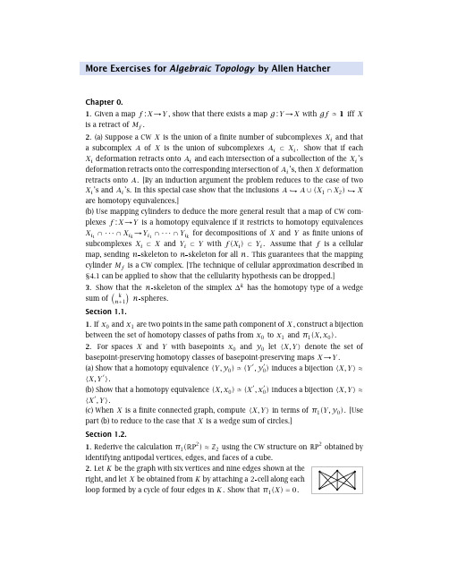
(b) X is the graph which is the suspension of n points and f is the suspension of a
cyclic permutation of the n points.
cylinder Mf is a CW complex. [The technique of cellular approximation described in §4.1 can be applied to show that the cellularity hypothesis can be dropped.]
3. Show that the n skeleton of the simplex ∆k has the homotopy type of a wedge
sum of
k n+1
n spheres.
Section 1.1.
1. If x0 and x1 are two points in the same path component of X , construct a bijection between the set of homotopy classes of paths from x0 to x1 and π1(X, x0) .
9. (a) Show that a finite CW complex, or more generally one with a finite 1 skeleton,
has finitely generated fundamental group.
(b) Show that a map f : X→Y with X compact and Y a CW complex cannot induce an
概率论与数理统计 习题4 英文版

EECE 7204
APPL. PROB. & STOCH. PROC.
Homework-4 Problem Set with Text
Due on October 18, 2011
2011 FALL
Reading Assignment: Chapter 4 from Stark and Woods, edition 4.
in part (a) above.
0.5
fX(x )
0.5
0
1
2
x
P4.9
Random variable X
is distributed according to the pd e−x u(x).
(a) Determine the mean µx = E [X ] of X . (b) Determine the variance σ2X = E X − µx 2 of X . (c) Determine the skewness of X given by
2x, 0 < x < 1, fX (x) = 0, else.
P4.2 Text Problem 4.18 (Page 285). Verify your answer in part (c) by computing the mean of the conditional mean determined in part (b). Let X and Y be two RVs. The pdf fX (x) of X is given as
P4.5 Text Problem 4.38 (Page 288).
Let X
be
a
uniform
- 1、下载文档前请自行甄别文档内容的完整性,平台不提供额外的编辑、内容补充、找答案等附加服务。
- 2、"仅部分预览"的文档,不可在线预览部分如存在完整性等问题,可反馈申请退款(可完整预览的文档不适用该条件!)。
- 3、如文档侵犯您的权益,请联系客服反馈,我们会尽快为您处理(人工客服工作时间:9:00-18:30)。
1 The Subgraph Bisimulation ProblemAgostino Dovier Carla PiazzaAbstractWe study the complexity of the Subgraph Bisimulation Problem,which stands to Graph Bisim-ulation as Subgraph Isomorphism stands to Graph Isomorphism and we prove its NP-Completeness.Our analysis is motivated by its applications to Semistructured Databases.Keywords:Bisimulation,Complexity,Semistructured DataI.I NTRODUCTIONGraph and Subgraph Isomorphism are two basic algorithmic problems[6].Although the latter is NP-complete,the lower bound for the time complexity of the former is still an open and very attractive issue.Bisimulation,a relation weaker than isomorphism,emerged as a fundamental property in various areas of Computer Science[1],[8].Polynomial time procedures can be used to check whether two distinct graphs are bisimilar[9].The Subgraph Bisimulation problem consists in identifying a subgraph Gof a graph G2bisimilar to a given graph G1.2The graphical query language G-log[10]uses this notion for retrieving data from semistruc-tured information[4].Data retrieval in the languages UnQL[2]and Graphlog[3]can be imple-mented on the basis of this notion,as shown in[5].Relationships between web-like databases and hypersets(where bisimulation is used for testing equivalence)are pointed out in[7].We prove that the Subgraph Bisimulation problem is NP-complete.As a consequence,data retrieval based on this notion in its generality is not feasible.However,a class of queries that allows polynomial time data retrieval based on Subgraph Bisimulation is shown in[5].A.Dovier is with the Dip.di Matematica e Informatica,Univ.di Udine.Via delle Scienze206,33100Udine(Italy).email: dovier@dimi.uniud.itC.Piazza is with the Dip.di Informatica,Univ.Ca’Foscari di Venezia.Via Torino155,30173Mestre—Venezia(Italy).email: piazza@dsi.unive.itII.B ASIC D EFINITIONS AND R ESULTSA directed graph (graph )is a pair G = N,E ,where N is the set of nodes and E ⊆N ×N is the set of edges.G 1= N 1,E 1 is a subgraph of G 2= N 2,E 2 if N 1⊆N 2and E 1⊆E 2.G 1= N 1,E 1 and G 2= N 2,E 2 are isomorphic (G 1≡G 2)if there exists a bijection f :N 1→N 2s.t.: u 1,v 1 ∈E 1⇔ f (u 1),f (v 1) ∈E 2.The Graph Isomorphism problem GI (G 1,G 2)amounts to determining whether G 1≡G 2;the Subgraph Isomorphism problem SI (G 1,G 2)consists in deciding whether there exists a subgraph G 2of G 2s.t.G 1≡G 2.A bisimulation [1]between G 1= N 1,E 1 and G 2= N 2,E 2 is a relation b ⊆N 1×N 2s.t.:(1)u 1∈N 1⇒∃u 2∈N 2(u 1b u 2),(2)u 2∈N 2⇒∃u 1∈N 1(u 1b u 2),(3)u 1b u 2∧ u 1,v 1 ∈E 1⇒∃v 2∈N 2(v 1bv 2∧ u 2,v 2 ∈E 2),(4)u 1bu 2∧ u 2,v 2 ∈E 2⇒∃v 1∈N 1(v 1bv 2∧ u 1,v 1 ∈E 1).If there is a bisimulation between G 1and G 2we say that G 1is bisimilar to G 2(G 1∼G 2).1The Graph Bisimulation problem GB (G 1,G 2)amounts to determining whether G 1∼G 2;the Subgraph Bisimulation problem SB (G 1,G 2)consists in deciding whether there exists a subgraph G 2of G 2s.t.G 1∼G 2.The problem GB (G 1,G 2)(GI (G 1,G 2))and the problem SB (G 1,G 2)(SI (G 1,G 2))are different.However,each graph isomorphism is a bisimulation.In Figure 1a bisimulation between two non isomorphic graphs is shown.u u u u u u 1u 2u 4u 3u 5E r r r j ¨¨¨B ¨¨¨B r r r j u u u u u v 1v 3v 2v 4v 5¨¨¨B r r r j r r r j ¨¨¨B E Fig.1.b ={ u 1,v 1 , u 2,v 2 , u 2,v 3 , u 3,v 4 , u 4,v 4 , u 5,v 5 }is a bisimulation between the two graphs.The size of an instance of each one of the problems is the sum of the number nodes and edges of G 1and G 2.The polynomiality of the GB problem follows from [9],where it is shown how to find the maximum bisimulation contraction in time O (|E |log |N |).1In [8]the notion is given on labeled graphs.The unlabeled notion of [1]is a particular case when all edges have the same label.Thus,NP hardness of the unlabeled version implies NP hardness of the labeled one.However,it can be shown that the labeled problem can be polynomially reduced to the unlabeled one.III.C OMPLEXITY R ESULTSSB (G 1,G 2)is in NP,since G 2∼G 1can be verified in polynomial time [9].We prove its NP-hardness by reducing the NP-complete Directed Hamilton Path (HP )problem 2([6],p.60)to SB.Let n ∈N ;C n = N,E is a n -chain if N ={x 1,...,x n }and E ={ x i +1,x i :1≤i <n }.Lemma 1:(i)If G = N,E ∼C n ,then |N |≥n .(ii)If G ∼C n and |N |=n ,then G ≡C n .Proof:The property (i)can be proved by induction on n ≥1.For (ii),let C n = {1,...,n },{ i +1,i :1≤i <n }and b a bisimulation between G and C n .We prove that b is a bijection from N to {1,...,n }.(1)states that b is defined on all nodes of N .We prove that b is a function.By contradiction,let i,j be the minimum pair (w.r.t.lexicographic order)s.t.∃n ∈N (y b i ∧y b j ∧i =j )(5).If y has no outgoing edges,by (4),i and j have no outgoing edges,i.e.i =j =1:a contradiction.Otherwise,let y,z ∈E .By (3),there are i ,j nodes of C n s.t. i,i and j,j are edges of C n and z b i and z b j .The form of C n ,however,implies that i =i −1and j =j −1.Hence, i,j is not the minimum pair satisfying the property(5):a contradiction.Thus,b is a function,and from (2)we know that b (N )={1,...,n },namely it is surjective.Since,by hypothesis and by the previous point,|N |=n =|b (N )|,b is also injective,and,thus,it is abijection.v v v v v E d d d ?-6-v v v v v E d d d c 'T 'v vv v v c E ''Fig.2.From left to right,the graph G admits a Hamilton path (‘thick’edges);G does not admit Hamilton paths;and C 5is a 5-chain (that trivially is a Hamilton path).Each Hamilton path on a 5-nodes graph is isomorphic (hence,bisimilar)to the 5-chain C 5.Theorem 1:The Subgraph Bisimulation problem is NP-complete.Proof:It remains to prove the NP-hardness of the problem.We reduce the HP problem to it.Let G = N,E ;we claim that HP (G )is equivalent to SB (C n ,G ),with C n a n -chain and n =|N |2HP (G )is the problem:given a graph G = N,E ,is there a path that visits each node of N exactly once?(see also Fig.2).Assume that G admits the Hamilton path:v n→v n−1→···→v1.By definition,the v i’s are pairwise distinct.Each edge occurring in the path occurs exactly once(otherwise,some node is repeated in the path).The path is a subgraph of G isomorphic(and hence bisimilar)to C n.Assume that there is a subgraph G of G bisimilar to C n.By Lemma1(i)G has at least n nodes;thus,being a subgraph of G,it has n nodes.By Lemma1(ii)G ≡C n,i.e.it is a n-chain describing a Hamilton path.The reduction is trivially in determisistic O(log n)space.Acknowledgements.We thank Elisa Quintarelli for the useful discussions concerning this work.R EFERENCES[1]P.Aczel.Non-well-founded sets.V ol.14of Lecture Notes,CLSI Stanford,1988.[2]P.Buneman,S.B.Davidson,G.G.Hillebrand,and D.Suciu.A Query Language and Opti-mization Techniques for Unstructured Data.In Proc.of the1996ACM SIGMOD,pp.505–516.[3]M.P.Consens and A.O.Mendelzon.Graphlog:a Visual Formalism for Real Life Recursion.In Proc.of9th ACM PODS’90,pp.404–416,1990.[4]A.Cortesi,A.Dovier,E.Quintarelli,and L.Tanca.Operational and Abstract Semantics of theQuery Language G-Log.Theoretical Computer Science,275(1–2):521–560,2002.[5]A.Dovier and E.Quintarelli:Model-Checking Based Data Retrieval.In Proc.of DatabaseProgramming Languages,8th Int.Workshop,LNCS V ol.2397,pp.62–77,2002.[6]M.R.Garey and puters and Intractability–A Guide to the Theory ofNP-Completeness.W.H.Freeman and Company,New York,1979.[7]A.Lisitsa and V.Sazonov.Bounded Hyperset Theory and Web-like Data Bases.In Proc.of5th Kurt G¨o del Colloquium,LNCS V ol.1289,pp.172–185,1997.[8]ner.Operational and Algebraic Semantics of Concurrent Processes.In Handbook ofTheoretical Computer Science,chapter19.Elsevier Science1990.[9]R.Paige and R.E.Tarjan.Three partition refinements algorithms.SIAM Journal on Comput-ing,16(6):973–989,1987.[10]J.Paredaens,P.Peelman,and L.Tanca.G-Log:A Declarative Graphical Query Language.IEEE Trans.on Knowledge and Data Eng.,7:436–453,1995.。
