Reliability Analysis of Multi-state Systems with S-dependent
舍不得说的PDF文件:Synopsys OptSim工具介绍说明书

DATASHEET Overview The Synopsys OptSim tool is an award-winning photonic integrated circuit and fiber-optic system simulator. With state-of-the-art time- and frequency-domain split-step algorithms, OptSim provides engineers around the globe with a native photonic-domain environment to design and optimize photonic circuits and systems. OptSim can be used as a standalone solution with its own graphical user interface (Windows and Linux), or integrated into the OptoCompiler Photonic IC design platform (Linux). When used as an OptoCompiler-integrated simulator, OptSim:•Supports electro-optic (E-O) co-simulation with Synopsys PrimeSim HSPICE and PrimeSim SPICE electrical circuit simulators •Integrates seamlessly with the PrimeWave Design Environment for advanced simulation, analyses, and visualization including parametric scans, Monte Carlo and corner analyses •Provides single- and multimode fiber-optic system modeling capabilities.When used as a standalone simulator, OptSim’s GUI provides functionalities of schematic entry, simulation setup, and visualization.Introduction Photonic integration is an answer to the ever-increasing demands for more bandwidth, better energy efficiency, smaller footprint, and improved reliability. The adaptation of photonic ICs (PICs) is rapidly growing acrossindustry segments such as telecom, data centers, optical interconnects,automotive, sensing, aerospace & defense, artificial intelligence (AI), andphotonic computing. PICs are becoming complex and the component count isincreasing at a rapid pace. Co-packaged optics (CPO) and xPU I/O are drivingmore complex trade-offs between electronics and photonics. Gone are the dayswhen it was sufficient to model photonics on the back of an envelope, withsome homegrown code, or as electronics in electrical circuit simulators. WithOptSim, you use the most comprehensive optical simulator with the industry’sbest electrical circuit simulators on the respective portions of the design withinthe OptoCompiler platform.Features at a Glance•E lectronic-photonic co-design via Synopsys PrimeSim HSPICE and PrimeSim SPICE•Simulation of single and multimode fiber optic systems and photonic integrated circuits•Seamless integration with OptoCompiler and PrimeWave Design Environment•Extensive libraries of photonic andelectronic components and analysistools•Support for numerous foundryprocess design kits (PDKs)•Support for custom photonics (PDKsand devices) via Photonic DeviceCompiler•Support for hierarchical design and bidirectional signal flow•Design for manufacturing via MonteCarlo and corner analyses OptSim Electro-Optic Co-Simulation of Photonic Integrated Circuits and Fiber-Optic SystemsDesigning single- and multimode fiber-optic systems requires capabilities to support advanced intensity- and phase-modulation for both single- and multi-channel transmission with direct and coherent detection. The interplay of polarization-dependent transmission impairments with noise, crosstalk, and multi-path interference (MPI) can create challenges to the channel capacity. In addition to PIC modeling capabilities, OptSim provides rich libraries of components and powerful analyses options to facilitate the design of a diverse range of system applications such as coherent telecom systems, RF-over-fiber, high-speed Ethernet, passive-optical-networks, and free-space optics.Figure 1: Photonic and electronic circuit and system simulation from the OptoCompiler cockpitFeatures•Works with foundry model libraries and provides a complete library of generic model templates of integrated photonics devices, enabling engineers to tailor models to measured behavior. In addition to supporting PIC design models and features, OptSim provides a rich library of single- and multimode fiber-optic system design models to support testing a PIC at the system levelFigure 2: The OptSim library includes electrical and photonic models to simulate circuits and systems•Models bidirectional signal flow for both optical (single- and multi-wavelength) and electrical signals•Models multipath interference (MPI), reflections, and resonances from network and PIC devices•Supports Monte Carlo and corner analyses•Supports simulation of design hierarchies•Supports measurement- and datafile-driven modeling of active and passive photonic components, electroniccomponents, and circuits•Supports custom design, combining foundry models and custom devices•Co-simulation with PrimeSim HSPICE and PrimeSim SPICE enables simulation of electronics in the PIC using industry-leading electrical circuit simulators together with the simulation of photonic circuits in OptSimFigure 3: Co-simulating electronic and photonic circuits in OptSim•OptSim is integrated with the Synopsys PrimeWave Design Environment, for both electrical and photonic netlists allowing setup of test benches, specifying simulation engine and parameters, performing scans and analyses for both electrical, photonic, and combined schematicsFigure 4: Setting up a testbench and simulation in PrimeWave Design Environment•OptSim results and waveforms (logical, electrical, and optical) can be viewed in both the PrimeWave Design Environment WaveView and OptSim Viewer©2021 Synopsys, Inc. All rights reserved. Synopsys is a trademark of Synopsys, Inc. in the United States and other countries. A list of Synopsys trademarks isavailable at /copyright .html . All other names mentioned herein are trademarks or registered trademarks of their respective owners.Figure 5: OptSim: Viewing simulation waveforms in PrimeWave Design Environment WaveView•Standalone OptSim (Windows, Linux) has its own graphical user interface and provides an intuitive simulation experienceFigure 6: OptSim GUI: Simulation of a PAM4 fiber-optic systemApplications:•Single- and multi-stage PICs for photonic computing, optical neural networks, life sciences, photonic sensor PICs •Segmented-electrode (SE) and traveling-wave Mach-Zehnder modulators (TW-MZM), optical filters, ring resonators,ring modulators•Transceivers for coherent and non-coherent fiber optic communication systems (such as NRZ, RZ, m-PAM, BPSK, QPSK,m-QAM, and OFDM)•Single- and multimode fiber-optic systems and circuits•Free-space optics, RF-over-fiber: Intermodulation distortion (IMD), dynamic range, sensitivity•Datacenter and automotive interconnects•Photonic systems with multipath interference (MPI), reflections, and resonancesPlatform Support•Linux: Red Hat Enterprise (64-bit), CentOS (64-bit)•Windows (64-bit): Standalone OptSim。
类圆曲线及其性质研究
5 结论本文提出了对含部件选择性失效传播的复杂可修系统进行可靠性与可用性计算的M C S C A 集成算法,给出了计算可靠性㊁瞬时可用性㊁区间可用性㊁平均维修时间以及平均单位时间维修次数五个指标的算法具体步骤,并最终通过实例具体说明了算法的应用㊂本文提出的算法解决了传统方法面临的两个主要问题,一是传统方法只能解决考虑部件选择性失效传播的简单系统可靠性问题,对于不能转化为串并联结构的复杂系统则无能为力,二是传统方法没有考虑系统的维修性,因此,对于复杂可修系统的可靠性与可用性评估传统方法也无从下手㊂本文提出的算法利用了计算机模拟的优势,并借鉴了具有并行计算能力的元胞自动机的思想,为含部件选择性失效传播的复杂可修系统的可靠性与可用性分析提供了一条有效的思路㊂参考文献:[1] L e v i t i nG,X i n g LD.R e l i a b i l i t y a n dP e r f o r m a n c eo fM u l t i s t a t e S y s t e m s w i t h P r o p a g a t e d F a i l u r e sH a v i n g S e l e c t i v eE f f e c t[J].R e l i a b i l i t y E n g i n e e r i n ga n dS y s t e mS a f e t y,2010,95(6):655‐661.[2] L e v i t i nG,X i n g LD,B e n‐H a i m H,e t a l.M u l t i‐s t a t eS y s t e m sw i t hS e l e c t i v eP r o p a g a t e dF a i l u r e s a n d I m-p e r f e c t I n d i v i d u a l a n dG r o u p P r o t e c t i o n s[J].R e l i a-b i l i t y E n g i n e e r i n g a n dS y s t e mS a f e t y,2011,96(12):1657‐1666.[3] G o b l eW M,B r o m b a c h e rAC,B u k o w s k i JV.U s i n gS t r e s s‐s t r a i nS i m u l a t i o n st o C h a r a c t e r i z eC o mm o nC a u s e[M].N e w Y o r k:S p r i n g e r,1998.[4] R o y D,D a s g u p t aT.A D i s c r e t i z i n g A p p r o a c h f o rE-v a l u a t i n g R e l i a b i l i t y o f C o m p l e x S y s t e m s u n d e rS t r e s s‐s t r e n g t h M o d e l[J].I E E E T r a n s a c t i o n so nR e l i a b i l i t y,2001,50(2):145‐150.[5] M y e r sA.K‐o u t‐o f‐N:GS y s t e m R e l i a b i l i t y w i t h I m-p e r f e c tF a u l tC o v e r a g e[J].I E E E T r a n s a c t i o n so nR e l i a b i l i t y,2007,56(3):464‐473.[6] X i n g L D.R e l i a b i l i t y E v a l u a t i o no fP h a s e d‐M i s s i o nS y s t e m sw i t hI m p e r f e c tF a u l tC o v e r a g ea n d C o m-m o n‐c a u s eF a i l u r e s[J].I E E ET r a n s a c t i o n s o nR e l i a-b i l i t y,2007,56(1):58‐68.[7] X i n g LD,D u g a n JB,M o r r i s s e t t eBA.E f f i c i e n tR e-l i a b i l i t y A n a l y s i so fS y s t e m s w i t h F u n c t i o n a lD e-p e n d e n c eL o o p s[J].M a i n t e n a n c ea n d R e l i a b i l i t y,2009,43(3):65‐69.[8] 王正,谢里阳,李兵,等.共因失效系统动态可靠性模型[J].中国机械工程,2008,19(1):5‐9.W a n g Z h e n g,X i eL i y a n g,L iB i n g,e ta l.T i m e‐d e-p e n d e n tR e l i a b i l i t y M o d e l o fS y s t e m w i t hC o mm o nC a u s eF a i l u r e[J].C h i n a M e c h a n i c a lE n g i n e e r i n g,2008,19(1):5‐9.[9] 李春洋,陈循,易晓山.考虑共因失效的多态系统可靠性优化[J].中国机械工程,2010,21(2):155‐159.L i C h u n y a n g,C h e n X u n,Y i X i a o s h a n.R e l i a b i l i t yO p t i m i z a t i o no f M u l t i‐s t a t eS y s t e mi nP r e s e n c eo fC o mm o nC a u s eF a i l u r e s[J].C h i n aM e c h a n i c a l E n g i-n e e r i n g,2010,21(2):155‐159.[10] W a n g C N,X i n g L D,L e v i t i nG.P r o p a g a t e dF a i l-u r eA n a l y s i s f o rN o n‐r e p a i r a b l e S y s t e m sC o n s i d e r-i n g B o t hG l o b a l a n dS e l e c t i v eE f f e c t s[J].R e l i a b i l i-t y E n g i n e e r i n g a n d S y s t e m S a f e t y,2012,99:96‐104.[11] 尹晓伟,钱文学,谢里阳.基于贝叶斯网络的系统可靠性共因失效模型[J].中国机械工程,2009,20(1):90‐94.Y i n X i a o w e i,Q i a n W e n x u e,X i eL i y a n g.C o mm o nC a u s eF a i l u r e M o d e lo fS y s t e m R e l i a b i l i t y B a s e do nB a y e s i a nN e t w o r k s[J].C h i n a M e c h a n i c a lE n g i-n e e r i n g,2009,20(1):90‐94.[12] A g g a r w a lK,G u p t aJ,M i s r aK.A S i m p l e M e t h o df o rR e l i a b i l i t y E v a l u a t i o n o f aC o mm u n i c a t i o nS y s-t e m[J].I E E E T r a n s a c t i o n so n C o mm u n i c a t i o n s,1975,23(5):563‐566.[13] Y e h W C.A R e v i s e dL a y e r e d‐n e t w o r k A l g o r i t h mt oS e a r c hf o r A l ld‐m i n p a t h so fa L i m i t e d‐f l o wA c y c l i cN e t w o k[J].I E E E T r a n s a c t i o n so n R e l i a-b i l i t y,1998,47(4):436‐442.[14] A v e n T.A v a i l a b i l i t y E v a l u a t i o no fO i l/G a sP r o-d u c t i o na n dT r a n s p o r t a t i o nS y s te m s[J].R e l i a b i l i t yE n g i n e e r i n g,1987,18(2):35‐44.[15] B i l l i n t o n R,A l l a n R N.R e l i a b i l i t y E v a l u a t i o no fE n g i n e e r i n g S y s t e m s,C o n c e p t s a n d T e c h n i q u e s[M].N e w Y o r k:P l e n u m P r e s s,1992. [16] F i s h m a nGS.A C o m p a r i s o no fF o u rM o n t eC a r l oM e t h o d s f o rE s t i m a t i n g t h eP r o b a b i l i t y o f s‐t C o n-n e c t e d n e s s[J].I E E E T r a n s a c t i o n so n R e l i a b i l i t y,1986,35(2):145‐155.[17] Y e h W C,L i nYC,C h u n g YY.P e r f o r m a n c eA n a l-y s i s o fC e l l u l a rA u t o m a t a M o n t eC a r l oS i m u l a t i o nf o r E s t i m a t i ng N e t w o r k R e l i a b i l i t y[J].E x p e r tS y s t e m s w i t h A p p l i c a t i o n s,2010,37(5):3537‐3544.[18] Z i o E,P o d o f i l l i n iL,Z i l l e V.A C o m b i n a t i o n o fM o n t eC a r l oS i m u l a t i o na n dC e l l u l a rA u t o m af o rC o m p u t i n g t h e A v a i l a b i l i t y o fC o m p l e x N e t w o r kS y s t e m s[J].R e l i a b i l i t y E n g i n e e r i n g a n d S y s t e mS a f e t y,2006,91(2):181‐190.[19] D e m i r S.R e l i a b i l i t y o fC o m b i n e dk‐o u t‐o f‐na n d㊃3231㊃存在共因失效的复杂可修系统可靠性评估 阮渊鹏 何 桢 张旭涛等Copyright©博看网. All Rights Reserved.C o n s e c u t i v ek (c )‐o u t ‐o f ‐nS y s t e m so fM a r k o vD e -p e n d e n tC o m p o n e n t s [J ].I E E ET r a n s a c t i o n so nR e -l i a b i l i t y,2009,58(4):691‐693.[20] G u oH T ,Y a n g X H.A u t o m a t i cC r e a t i o n o fM a r k -o v M o d e l s f o rR e l i a b i l i t y A s s e s s m e n t o f S a f e t y I n -s t r u m e n t e d S y s t e m s [J ].R e l i a b i l i t y E n g i n e e r i n g a n dS y s t e mS a f e t y,2008,93(6):829‐837.[21] X i a oG ,L i ZZ .E s t i m a t i o no fD e p e n d a b i l i t y M e a s -u r e s a n dP a r a m e t e r S e n s i t i v i t i e s o f aC o n s e c u t i v e ‐k‐o u t ‐o f ‐n :F R e p a i r a b l eS y s t e m w i t h (k-1)‐s t e p M a r k o v D e p e n d e n c e b y S i m u l a t i o n [J ].I E E E T r a n s a c t i o n s o nR e l i a b i l i t y ,2008,57(1):71‐83.[22] M a r q u e z A C ,H e g u e d a s A S ,L u n g B .M o n t e C a r l o ‐b a s e d A s s e s s m e n t o f S y s t e m A v a i l a b i l i t y[J ].R e l i a b i l i t y E n g i n e e r i n g a n d S y s t e m S a f e t y,2005,88(3):273‐289.[23] D u r g oR a oK ,G o p i k aV ,S a n ya s i R a oV VS ,e t a l .D y n a m i cF a u l tT r e e A n a l y s i s U s i n g Mo n t eC a r l o S i m u l a t i o n i nP r o b a b i l i s t i cS a f e t y A s s e s s m e n t [J ].R e l i a b i l i t y E n g i n e e r i n g a n dS y s t e mS a f e t y ,2009,94(4):872‐883.(编辑 王艳丽)作者简介:阮渊鹏,男,1985年生㊂天津大学管理与经济学部博士研究生,杭州电子科技大学管理学院讲师㊂主要研究方向为质量与可靠性工程㊂发表论文8篇㊂何 桢,男,1967年生㊂天津大学管理与经济学部教授㊁博士研究生导师㊂张旭涛,1981年生㊂天津大学管理与经济学部博士研究生,军事交通学院装备保障系讲师㊂张 驰,1988年生㊂天津大学管理与经济学部博士研究生㊂类圆曲线及其性质研究陈 明 刘延平哈尔滨工业大学,哈尔滨,150001摘要:对偏心圆节曲线非圆齿轮传动和椭圆节曲线非圆齿轮传动的关键设计参数偏心率e 和离心率ε分别进行了分析㊂在椭圆曲线的基础上,通过改变极坐标极点,得到了一种新型的封闭曲线类圆曲线,它可以看作是更广义的椭圆曲线或偏心圆曲线㊂针对一般意义的椭圆曲线和偏心圆曲线只是类圆曲线的两种特殊类型的情况,在类圆曲线的数学表达式中,引入了两个关键设计参数偏心率e 和离心率ε,建立了具有不同性质的非圆齿轮节圆曲线方程㊂研究发现,偏心率e 可以确定类圆曲线的最小和最大向径,离心率ε可以确定类圆曲线的形状㊂类圆曲线非圆齿轮传动具有与偏心圆齿轮和椭圆齿轮类似的传动特点,同时在设计上比偏心圆齿轮和椭圆齿轮更加灵活㊁方便㊂关键词:类圆曲线;偏心圆节曲线;椭圆节曲线;非圆齿轮中图分类号:T H 3 D O I :10.3969/j.i s s n .1004-132X.2014.10.010S t u d y o n Q u a s i -c i r c u l a rC u r v e a n d I t s P r o pe r t i e s C h e n M i n g L i uY a n p i n gH a r b i n I n s t i t u t e o fT e c h n o l o g y,H a r b i n ,150001A b s t r a c t :T h i s p a p e r s t u d i e d t h e k e y d e s i g n p a r a m e t e r s ,t h e e c c e n t r i c i t yr a t i o e o f e c c e n t r i c c i r c u l a r c u r v e a n d t h e e c c e n t r i c i t y εo f e l l i p t i c c u r v e ,w h i c hw e r eu s e dc o mm o n l y f o rn o n ‐c i r c u l a r g e a r t r a n s -m i s s i o n .B y c h a n g i n g t h e p o l e o f t h e p o l a r c o o r d i n a t e s ,an e wt r a n s f o r m e de l l i pt i c c u r v en a m e d q u a s i ‐c i r c u l a r c u r v e c a nb e o b t a i n e d ,w h i c h c a nb e r e g a r d e d a s g e n e r a l i z e d e l l i p t i c c u r v e o r g e n e r a l i z e d e c c e n -t r i c c u r v e .A i m i n g a t t h a t t h eo r i g i n a l e l l i p t i c c u r v e a n de c c e n t r i c c u r v ew e r e j u s t s pe c i a l c a s e sof t h e q u a s i ‐c i r c u l a r c u r v e ,t w ok e y d e s ig n p a r a m e t e r s ,e c c e n t r i c i t y ra t i o e a n de c c e n t r i c i t y εw e r e i n t r o d u c e d i n t o t h em a t h e m a t i c a l e x p r e s s i o no f t h e q u a s i ‐c i r c u l a r c u r v e t ob u i l dan e we x p r e s s i o no f t h e p i tc ho f n o n ‐c i r c u l a r g e a r .T h e r e s e a r c h i nd i c a te s t h a t t h ee c c e n t r i c i t y r a t i od e t e r m i n e s t h em i n i m u ma n d t h e m a x i m u mr a d i u s of t h e q u a s i ‐c i r c u l a r c u r v e a n d t h e e c c e n t r i c i t y d e t e r m i n e s t h e s h a p e o f t h e q u a s i ‐c i r -c u l a r c u r v e .T h e q u a s i ‐c i r c u l a r ge a r t r a n s m i s s i o n h a s t h e c h a r a c t e r i s t i c s s i m i l a r t o t h e e c c e n t r i c c i r c u l a r g e a r s a n de l l i p t i c g e a r s ,b u t i t i sm o r ef l e x i b l e a n d c o n v e n i e n t t od e s i gn .K e y wo r d s :q u a s i ‐c i r c u l a r c u r v e ;e c c e n t r i c c i r c u l a r g e a r ;e l l i p t i c g e a r ;n o n ‐c i r c u l a r g e a r 0 引言偏心圆节曲线非圆齿轮传动和椭圆节曲线非收稿日期:2012 10 08圆齿轮传动在机械系统中常常分别作为典型传动形式应用[1‐3]㊂但是,从几何学的角度来看,偏心圆和椭圆之间有着密切的渊源关系㊂通过研究椭㊃4231㊃中国机械工程第25卷第10期2014年5月下半月Copyright ©博看网. All Rights Reserved.圆和偏心圆曲线之间的渊源关系,可以揭示与椭圆和偏心圆曲线具有统一数学表达形式的一族曲线的性质㊂为了叙述方便,把这一族曲线称为 类圆曲线”㊂把 类圆曲线”应用到非圆齿轮传动中,可以使非圆齿轮传动的设计更加方便和灵活㊂1 偏心圆㊁椭圆节曲线的数学模型1.1 偏心圆齿轮的节曲线图1 偏心圆齿轮的节曲线图1所示为偏心圆齿轮的节曲线㊂点C 是该节曲线的圆心,点O 1是偏心圆齿轮的回转中心,a 是该节曲线的半径,r 1是该节曲线的向径㊂该偏心圆齿轮的偏心距为E =O 1C(1)由此,可以写出偏心圆齿轮节曲线的极坐标方程[4]:r 1=a 2-E 2s i n 2φ1-E c o s φ1(2)为了研究问题方便,经常把式(2)写成以下形式:r 1=a (1-e 2s i n 2φ1-e c o s φ1)(3)式中,e 为偏心率,e =E a㊂偏心圆齿轮的节曲线虽然从形状上看是一个圆,但是节曲线上的各点到回转中心的距离不相同㊂当偏心圆齿轮与另外一个齿轮啮合,中心距为常数时,这个齿轮的节曲线为非圆曲线,这两个齿轮的速比也不是常数㊂因此,偏心圆齿轮在传动中所表现出来的特征与非圆齿轮相同㊂为叙述方便,把非圆齿轮节曲线上距离回转中心最近的点称为节曲线的 近端点”,距离回转中心最远的点称为节曲线的 远端点”㊂1.2 变形偏心圆曲线把偏心圆齿轮节曲线的极坐标方程(式(2))写成如下形式:r 1=a [1-e 2s i n 2(n 1φ1)-e c o s (n 1φ1)](4)式中,n 1为变形偏心圆曲线的叶(支)数,为正整数㊂显然,该函数周期为2π/n 1[4]㊂当n 1=1时,式(4)与式(3)一样,所表达的是一个偏心圆㊂当n 1>1时,式(4)所表达的曲线称为变形偏心圆㊂图2为n 1=3时的变形偏心圆曲线,图3㊁图4分别为相应的相对向径(r 1/a )和相对曲率(a /ρ1)变化曲线㊂如图2~图4所示,随着偏心率的增大,变形偏心圆曲线的叶形变得越来越扁长,变形偏心圆的最大向径增大而其最小向径减小;当偏心率为零时,变形偏心圆曲线的相对曲率(a /ρ1)为常数1,也就是说,此时变形偏心圆是一个圆㊂随着偏心率的增大,变形偏心圆曲线的相对曲率(a /ρ1)发生较大变化,偏心率越大,相对曲率变化越剧烈㊂在最大向径(远端)附近,相对曲率变化较平缓,在最小向径(近端)附近,相对曲率变化较剧烈㊂1.e =02.e =0.23.e =0.44.e =0.65.e =0.8图2 偏心率对变形偏心圆曲线(n 1=3)的影响1.e =0 2.e =0.2 3.e =0.4 4.e =0.6 5.e =0.8图3 变形偏心圆曲线(n 1=3)的相对向径1.e =0 2.e =0.2 3.e =0.4 4.e =0.6 5.e =0.8图4 变形偏心圆曲线(n 1=3)的相对曲率1.3 椭圆齿轮的节曲线图5所示是椭圆齿轮的节曲线,点C 是椭圆曲线的几何中心,点O 1是椭圆曲线的焦点也是椭圆齿轮的回转中心,a 是椭圆曲线的长半轴,b 是椭圆曲线的短半轴,c 是椭圆曲线的焦距㊂选焦点O 1为极坐标的极点,O 1p 为极坐标的极轴,则椭圆曲线的极坐标方程为[5]r 1=a (1-ε2)1+εc o s φ1(5)ε=ca =a 2-b 2a㊃5231㊃类圆曲线及其性质研究陈 明 刘延平Copyright ©博看网. All Rights Reserved.图5 椭圆齿轮的节曲线式中,ε为离心率㊂椭圆曲线是非圆齿轮传动中常用的一种节曲线,可以实现主动轮与从动轮节曲线相同的共轭传动[6‐7]㊂这在非圆齿轮传动中是不多见的㊂1.4 变形椭圆曲线把椭圆齿轮节曲线的极坐标方程(式(5))写成如下形式[8]:r 1=a (1-ε2)1+εc o s (n 1φ1)(6)式中,n 1为变形椭圆曲线的叶(支)数,为正整数㊂显然,该函数周期为2π/n 1㊂当n 1=1时,式(6)与式(5)一样,表达的是一个椭圆㊂椭圆曲线离心率越大,相对曲率的变化越剧烈,其近端和远端的相对曲率也越大㊂当n 1>1时,式(6)所表达的曲线称为变形椭圆曲线(即卵形曲线)㊂当n 1=3时,对应不同离心率的变形椭圆曲线如图6所示,变形椭圆曲线的相对向径(r 1/a )和相对曲率(a /ρ1)变化分别如图7㊁图8所示㊂由图6可以看出,随着离心率的增大,变形椭圆曲线的叶形变得越来越扁长;由图7可以看出,随着离心率的增大,变形椭圆曲线的最大向径增大而其最小向径减小;由图8可以看出,当离心率ε=0时,变形椭圆曲线的相对曲率(a /ρ1)为常数1,此时变形椭圆实际上是一个圆㊂随着离心率的增大,变形椭圆曲线的相对曲率(a /ρ1)发生较大变化,离心率越大,相对曲率变化越剧烈㊂在最大相对向径附近(远端),相对曲率变化较剧烈,在最小相对向径附近(近端),相对曲率变化较平缓㊂1.ε=02.ε=0.23.ε=0.44.ε=0.65.ε=0.8图6 离心率对变形椭圆曲线(n 1=3)的影响1.ε=0 2.ε=0.2 3.ε=0.4 4.ε=0.6 5.ε=0.8图7 变形椭圆曲线(n 1=3)的相对向径1.ε=0 2.ε=0.2 3.ε=0.4 4.ε=0.6 5.ε=0.8图8 变形椭圆曲线(n 1=3)的相对曲率2 偏心圆线与椭圆曲线性质的对比由上文分析可知,影响偏心圆曲线相对向径的关键因素是偏心圆曲线的偏心率e ,影响椭圆曲线相对向径的关键因素是椭圆曲线的离心率ε㊂因此,可以说影响偏心圆齿轮传动比的关键因素是其偏心率e ,影响椭圆齿轮传动比的关键因素是其离心率ε㊂非圆齿轮传动比的计算公式为[9]i =A -r 1r 1(7)式中,A 为非圆齿轮传动的中心距;r 1为主动轮节曲线向径;i 为传动比㊂传动比的最大值发生在主动轮的近端点,即i m a x =A -r m i n 1r m i n 1(8)传动比的最小值发生在主动轮的远端点,即i m i n =A -r m a x 1r m a x 1(9)最大最小传动比差值为Δi =i m a x -i m i n =A (r m a x 1-r m i n 1)r m i n 1r m a x 1(10)对于偏心圆节曲线,根据式(3),得到其最大向径为r m a x 1=a (1+e )(11)最小向径为r m i n 1=a(1-e )(12)把式(11)㊁式(12)代入式(10)得偏心圆齿轮传动的最大最小传动比差为㊃6231㊃中国机械工程第25卷第10期2014年5月下半月Copyright ©博看网. All Rights Reserved.Δi=2A ea(1-e2)(13)对于椭圆节曲线,根据式(5),得到其最大向径为r m a x1=a(1+ε)(14)最小向径为r m i n1=a(1-ε)(15)把式(14)㊁式(15)代入式(10)得椭圆齿轮传动的最大最小传动比差为Δi=2Aεa(1-ε2)(16)由式(13)㊁式(16)可以看出,偏心圆齿轮传动和椭圆齿轮传动的最大最小传动比差分别受到偏心率和离心率的影响,并且这种影响程度是相同的㊂但是,偏心圆齿轮传动的偏心率e仅影响传动比,不影响偏心圆节曲线的形状;而椭圆齿轮传动的离心率ε不仅影响其传动比,还影响椭圆节曲线的形状[10]㊂3 变形偏心圆曲线与变形椭圆曲线性质的对比通过对1.2节中变形偏心圆曲线与1.4节中变形椭圆曲线的性质进行对比可以发现,两种曲线的性质既有相同点又有差异,具体如表1所示㊂表1 变形偏心圆与变形椭圆曲线性质对比相同点叶数n1等于曲线远端点数目和近端点数目远端点极角φ1=180°n1+(j-1)360°n1j=1,2, ,n1近端点极角φ1=(j-1)360°n1j=1,2, ,n1曲线的向径变化趋势在变形偏心圆曲线与变形椭圆曲线的远端点和近端点之间,曲线的向径均为单调增大或单调减小偏心率e(离心率ε)对远近端的影响随着e(ε)的增大,变形偏心圆曲线(变形椭圆曲线)的远端越远,近端越近偏心率e(离心率ε)对相对曲率的影响随着e(ε)的增大,变形偏心圆曲线(变形椭圆曲线)的远端相对曲率增大,近端相对曲率由正变负,且其绝对值越来越大偏心率e(离心率ε)对叶形的影响变形偏心圆曲线(变形椭圆曲线)的e(ε)越大,曲线的叶形越扁长㊂不同点偏心率e(离心率ε)对相对曲率变化率的影响随着e的增大,变形偏心圆曲线的远端相对曲率变化较平缓并变得更加丰满圆润,近端相对曲率变化剧烈㊂随着ε的增大,变形椭圆曲线的远端相对曲率变化剧烈并急剧变尖,近端相对曲率变化较为平缓㊂通过对比变形偏心圆曲线和变形椭圆曲线的性质发现,在偏心率e较大时,变形偏心圆曲线的近端凹陷较剧烈,致使变形偏心圆曲线不能用作非圆齿轮的节曲线;在离心率ε较大时,变形椭圆曲线的远端变尖较剧烈,致使变形椭圆曲线不能用作非圆齿轮的节曲线㊂如果能够把变形偏心圆曲线和变形椭圆曲线的这种性质综合在一起,得到一种新型曲线,使得偏心率e或离心率ε较大时,曲线的远端变化类似变形偏心圆曲线,而曲线的近端变化类似变形椭圆曲线,那么这种新型曲线将会给非圆齿轮节曲线的设计带来很大的方便性和灵活性[11]㊂4 类圆曲线的数学模型图9所示为椭圆曲线,点O是椭圆曲线的几何中心,点C1㊁点C2是椭圆曲线的焦点,点O1是椭圆齿轮的回转中心,a是椭圆曲线的长半轴,b图9 椭圆齿轮的节曲线是椭圆曲线的短半轴,c是椭圆曲线的焦距,E是椭圆齿轮的偏心距㊂选回转中心O1为极坐标的极点,O1p为极坐标的极轴,则椭圆曲线的极坐标方程为r1=a(1-ε2)(1-ε2c o s2φ1-e2s i n2φ1)1-ε2c o s2φ1-a e(1-ε2)c o sφ11-ε2c o s2φ1(17)当令式(17)中的离心率ε=0时,则式(17)退化成式(3);当令式(17)中的偏心率e=ε时,则式(17)退化成式(5)㊂由此可见,偏心圆曲线和椭圆曲线是式(17)的特殊情况;当式(17)中ε≠0,e≠ε时,式(17)所表示的曲线具有偏心圆曲线和椭圆曲线均不具备的特性㊂由于式(17)所表达的曲线与偏心圆曲线和椭圆曲线既有渊源关系又有不同的特性,因此,把这类曲线称为类圆曲线㊂实际上,当式(17)中ε=0,e=0时,式(17)所表达的曲线是一个圆㊂类圆曲线也可以像偏心圆曲线和椭圆曲线那样,在其表达式的自变量前乘以一个正整数以实现变形,其表达式为㊃7231㊃类圆曲线及其性质研究 陈 明 刘延平Copyright©博看网. All Rights Reserved.r 1=a(1-ε2)[1-ε2c o s 2(n 1φ1)-e 2s i n 2(n 1φ1)]1-ε2c o s 2(n 1φ1)-a e (1-ε2)c o s (n 1φ1)1-ε2c o s 2(n 1φ1)(18)当n 1=1时,式(18)与式(17)所表达的曲线相同㊂当偏心率e =0,离心率ε=0㊁0.4㊁0.6㊁0.7㊁0.8时,类圆曲线如图10所示,类圆曲线的相对向径(r 1/a )变化如图11所示,类圆曲线的相对曲率(a /ρ1)变化如图12所示㊂由图10可以看出,随着离心率的增大,类圆曲线变得越来越扁,且极坐标系的极点O 1在曲线的几何中心㊂由图11可以看出,类圆曲线的最大相对向径出现在极角φ1=0°和180°时,并且最大相对向径不随离心率ε的变化而变化;类圆曲线的最小相对向径出现在极角φ1=90°和270°时,并且最小相对向径随离心率ε的增大而减小㊂由图12可以看出,类圆曲线的最大相对向径处的相对曲率,随着离心率ε的增大而增大;类圆曲线的最小相对向径处的相对曲率,随着离心率ε的增大而减小㊂由图10~图12可以看出,当离心率ε=0时,类圆曲线实际上就是一个圆㊂因此可以说,圆是类圆曲线的一种特殊情况㊂1.ε=02.ε=0.23.ε=0.44.ε=0.65.ε=0.8图10 离心率对类圆曲线(n 1=1,e =0)的影响1.ε=0 2.ε=0.2 3.ε=0.4 4.ε=0.6 5.ε=0.8图11 类圆曲线(n 1=1,e =0)的相对向径当n 1=1,偏心率e =0.2,离心率分别取ε=0㊁0.4㊁0.6㊁0.7㊁0.8时,类圆曲线如图13所示,类圆曲线的相对向径(r 1/a )变化如图14所示,类圆曲线的相对曲率(a /ρ1)变化如图15所示㊂由图13可以看出,随着离心率的增大,类圆曲线变得越来1.ε=0 2.ε=0.2 3.ε=0.4 4.ε=0.6 5.ε=0.8图12 类圆曲线(n 1=1,e =0)的相对曲率1.ε=0 2.ε=0.2 3.ε=0.4 4.ε=0.6 5.ε=0.8图13 离心率对类圆曲线(n 1=1,e =0.2)的影响1.ε=0 2.ε=0.2 3.ε=0.4 4.ε=0.6 5.ε=0.8图14 类圆曲线(n 1=1,e =0.2)的相对向径1.ε=0 2.ε=0.2 3.ε=0.4 4.ε=0.6 5.ε=0.8图15 类圆曲线(n 1=1,e =0.2)的相对曲率越扁,且极坐标系的极点O 1偏离曲线的几何中心㊂由图14可以看出,类圆曲线的最小相对向径在离心率ε较小时,出现在极角φ1=0°时,但是,随着离心率ε的增大,最小相对向径出现的位置发生了变化;类圆曲线的最大相对向径出现在极角φ1=180°时,并且最大相对向径不随离心率ε的变化而变化㊂由图15可以看出,类圆曲线的最㊃8231㊃中国机械工程第25卷第10期2014年5月下半月Copyright ©博看网. All Rights Reserved.大相对向径附近的相对曲率,随着离心率ε的增大而增大,最小相对向径附近的相对曲率,随着离心率ε的增大而减小㊂由图13~图15可以看出,当离心率ε=0时,类圆曲线实际上就是一个偏心圆㊂通过对上述两种单叶(n 1=1)类圆曲线的分析可知,上述两种类圆曲线实际上都是椭圆曲线㊂只不过描述这两种椭圆曲线的极坐标系的极点O 1不像通常那样处在椭圆的焦点上,而是处在椭圆的长轴上,其到椭圆几何中心的距离为a e (椭圆长半轴a 与偏心率e 的乘积)㊂所谓类圆曲线实质上是在椭圆曲线的数学表达式中引入了新的参数 偏心率e ,用偏心率e 描述极坐标系极点到其几何中心的距离,而离心率ε则只用来描述椭圆曲线的形状,即椭圆 扁”的程度㊂而普通椭圆曲线只有一个参数离心率ε,它不仅用来描述椭圆 扁”的程度,还要用来描述椭圆曲线极坐标系极点到其几何中心的距离㊂当n 1=2,偏心率e =0,离心率ε=0㊁0.4㊁0.6㊁0.7㊁0.8时,类圆曲线如图16所示,类圆曲线的相对向径(r 1/a )变化如图17所示,类圆曲线的相对曲率(a /ρ1)变化如图18所示㊂由图16可以看出,随着离心率的增大,类圆曲线的叶形变得越来越扁,且极坐标系的极点O 1位于曲线的几何中心㊂由图17可以看出,类圆曲线的最小相对向径出现在极角φ1=45°㊁135°㊁225°㊁315°时,且最小相对向径随着随离心率ε的增大而减小;类圆曲线的最大相对向径出现在极角φ1=0°㊁90°㊁180°㊁270°时,并且最大相对向径不随离心率ε的变化而变化㊂由图18可以看出,类圆曲线的最大相对向径附近的相对曲率,随着离心率ε的增大而增大,最小相对向径附近的相对曲率,随着离心率ε的增大而减小㊂由图16~图18可以看出,当离心率ε=0时,类圆曲线实际上就是一个偏心圆㊂1.ε=02.ε=0.23.ε=0.44.ε=0.65.ε=0.8图16 离心率对类圆曲线(n 1=2,e =0)的影响当n 1=2,偏心率e =0.2,离心率ε=0㊁0.4㊁0.6㊁0.7㊁0.8时,类圆曲线如图19所示,类圆曲线1.ε=0 2.ε=0.2 3.ε=0.4 4.ε=0.6 5.ε=0.8图17 类圆曲线(n 1=2,e =0)的相对向径1.ε=0 2.ε=0.2 3.ε=0.4 4.ε=0.6 5.ε=0.8图18 类圆曲线(n 1=2,e =0)的相对曲率的相对向径(r 1/a )变化如图20所示,类圆曲线的相对曲率(a /ρ1)变化如图21所示㊂由图19可以看出,随着离心率的增大,类圆曲线的叶形变得越来越扁,且极坐标系的极点O 1位于曲线的几何中心㊂由图20可以看出,在离心率ε较小时,类圆曲线的最小相对向径出现在极角φ1=0°和180°时;但是,随着离心率ε的增大,最小相对向径出现的位置发生了变化;类圆曲线的最大相对向径出现在极角φ1=90°和270°时,并且最大相对向径不随离心率ε的变化而变化㊂由图21可以看出,类圆曲线的最大相对向径附近的相对曲率随着离心率ε的增大而增大,最小相对向径附近的相对曲率,随着离心率ε的增大而减小㊂1.ε=0 2.ε=0.2 3.ε=0.4 4.ε=0.6 5.ε=0.8图19 离心率对类圆曲线(n 1=2,e =0.2)的影响当n 1=3,偏心率e =0,离心率ε=0㊁0.4㊁0.6㊁0.7㊁0.8时,类圆曲线如图22所示,类圆曲线的相对向径(r 1/a )变化如图23所示,类圆曲线的相对曲率(a /ρ1)变化如图24所示㊂由图22可以看出,随着离心率的增大,类圆曲线的叶形变得越来㊃9231㊃类圆曲线及其性质研究陈 明 刘延平Copyright ©博看网. All Rights Reserved.1.ε=02.ε=0.23.ε=0.44.ε=0.65.ε=0.8图20 类圆曲线(n 1=2,e =0.2)的相对向径1.ε=0 2.ε=0.2 3.ε=0.4 4.ε=0.6 5.ε=0.8图21 类圆曲线(n 1=2,e =0.2)的相对曲率越扁,且极坐标系的极点O 1位于曲线的几何中心㊂由图23可以看出,类圆曲线的最小相对向径出现在极角φ1=30°㊁90°㊁150°㊁210°㊁270°㊁330°时,且最小相对向径随着随离心率ε的增大而减小;类圆曲线的最大相对向径出现在极角φ1=0㊁60°㊁120°㊁180°㊁240°㊁300°时,并且最大相对向径不随离心率ε的变化而变化㊂由图24可以看出,类圆曲线的最大相对向径附近的相对曲率,随着离心率ε的增大而增大,最小相对向径附近的相对曲率,随着离心率ε的增大而减小㊂由图22~图24可以看出,当离心率ε=0时,类圆曲线实际上就是一个偏心圆㊂1.ε=02.ε=0.23.ε=0.44.ε=0.65.ε=0.8图22 离心率对类圆曲线(n 1=3,e =0)的影响当n 1=3,偏心率e =0.2,离心率ε分别取0㊁0.4㊁0.6㊁0.7㊁0.8时,类圆曲线如图25所示,类圆曲线的相对向径(r 1/a )变化如图26所示,类圆曲线的相对曲率(a /ρ1)变化如图27所示㊂由图251.ε=0 2.ε=0.2 3.ε=0.4 4.ε=0.6 5.ε=0.8图23 类圆曲线(n 1=3,e =0)的相对向径1.ε=0 2.ε=0.2 3.ε=0.4 4.ε=0.6 5.ε=0.8图24 类圆曲线(n 1=3,e =0)的相对曲率可以看出,随着离心率的增大,类圆曲线的叶形变得越来越扁,且极坐标系的极点O 1位于曲线的几何中心㊂由图26可以看出,在离心率ε较小时,类圆曲线的最小相对向径出现在极角φ1=0°㊁120°㊁240°时;但是,随着离心率ε的增大,最小相对向径出现的位置发生了变化;类圆曲线的最大相对向径出现在极角φ1=60°㊁180°㊁300°时,并且最大相对向径不随离心率ε的变化而变化㊂由图27可以看出,类圆曲线的最大相对向径附近的相对曲率随着离心率ε的增大而增大,最小相对向径附近的相对曲率随着离心率ε的增大而减小㊂1.ε=02.ε=0.23.ε=0.44.ε=0.65.ε=0.8图25 离心率对类圆曲线(n 1=3,e =0.2)的影响由上述分析可知,类圆曲线的最大相对向径的位置只与类圆曲线的叶数n 1有关,与离心率ε无关,可以称相对向径最大处为类圆曲线的远端㊂类圆曲线的最小相对向径的位置不仅与类圆曲线的叶数n 1有关,还与离心率ε有关㊂为了研㊃0331㊃中国机械工程第25卷第10期2014年5月下半月Copyright ©博看网. All Rights Reserved.1.ε=02.ε=0.23.ε=0.44.ε=0.65.ε=0.8图26 类圆曲线(n1=3,e=0.2)的相对向径1.ε=02.ε=0.23.ε=0.44.ε=0.65.ε=0.8图27 类圆曲线(n1=3,e=0.2)的相对曲率究问题方便,把离心率ε较小时的相对向径最小处称为类圆曲线的准近端,类圆曲线相对向径最小处称为类圆曲线的近端㊂综上所述,得到类圆曲线的性质如下: (1)类圆曲线的叶数n1分别等于曲线远端点数目和准近端点数目㊂(2)类圆曲线的远端点极角为φ1=180°n1+(j-1)360°n1(19)j=1,2, ,n1准近端点极角为φ1=(j-1)360°n1(20)j=1,2, ,n1(3)当离心率ε较小时,在类圆曲线的远端点和准近端点之间,曲线的相对向径是单调增大或单调减小的㊂随着离心率ε的增大,在类圆曲线的远端点和准近端点之间,曲线的相对向径不再单调增大或单调减小㊂(4)类圆曲线的远端点和准近端点不随离心率ε的变化而变化㊂(5)随着离心率ε的增大,类圆曲线的远端相对曲率增大,准近端相对曲率也增大,而其近端相对曲率由正变负,且其绝对值越来越大㊂(6)类圆曲线的离心率ε越大,曲线叶形越扁㊂(7)随着离心率ε的变化,类圆曲线的远端和准近端相对曲率的变化程度相近㊂根据上述分析,总结偏心圆曲线㊁椭圆曲线和类圆曲线的性质见表2㊂表2 偏心圆㊁椭圆㊁类圆曲线性质项目曲线类型偏心圆曲线椭圆曲线类圆曲线偏心距e有无有离心率ε无有有(准)近端位置φ1=(j-1)360°n1j=1,2, ,n近端位置与上相同与上相同与上不同远端位置φ1=180°n1+(j-1)360°n1j=1,2, ,n向径变化规律曲率变化规律近端→远端近端→远端准近端→远端单调增大单调增大ε较小时单调增大近端→远端近端→远端准近端→远端单调减小单调减小ε较小时单调减小近端近端准近端剧烈减小平缓减小较平缓增大远端远端远端平缓增大剧烈增大较平缓增大 把类圆曲线的远端点极角表达式(式(19))代入类圆曲线表达式(式(18))得类圆曲线的最大向径为r m a x1=a(1+e)(21)把准近端点极角表达式(式(20))代入类圆曲线表达(式(18))得类圆曲线的最小向径为r m i n1=a(1-e)(22)则类圆曲线作为节曲线的非圆齿轮传动的最大最小传动比差为Δi=2A ea(1-e2)(23)对比图22和图25可以看出,非圆齿轮类圆节曲线的最大向径只与偏心率e有关,与离心率ε无关;而其最小向径不仅与偏心率e有关,同时也受离心率ε的影响㊂同时,由式(23)也可以看出,类圆齿轮传动的最大最小传动比差主要受偏心率e的影响,离心率ε对其影响较小(式(23)中的中心距A与离心率ε有关)㊂这样,在设计类圆节曲线非圆齿轮时,可以通过改变偏心率e和离心率ε来确定类圆曲线的最小㊁最大向径及类圆曲线的形状,满足非圆齿轮的最大㊁最小传动比要求和非圆齿轮的传动比变化规律或非圆齿轮节曲线形状的要求㊂类圆节曲线非圆齿轮的设计,要比偏心㊃1331㊃类圆曲线及其性质研究 陈 明 刘延平Copyright©博看网. All Rights Reserved.。
计算机英文文献加翻译

Management Information System Overview Management Information System is that we often say that the MIS, is a human, computers and other information can be composed of the collection, transmission, storage, maintenance and use of the system, system, emphasizing emphasizing the the management, management, management, stressed stressed stressed that that the modern information society In the increasingly popular. MIS is a new subject, it across a number of areas, such as scientific scientific management management management and and and system system system science, science, science, operations operations operations research, research, research, statistics statistics statistics and and and computer computer science. In these subjects on the basis of formation of information-gathering and processing methods, thereby forming a vertical and horizontal weaving, and systems. The 20th century, along with the vigorous development of the global economy, many economists have proposed a new management theory. In the 1950s, Simon made dependent on information management and decision-making ideas. Wiener published the same period of the control theory, that he is a management control process. 1958, Gail wrote: "The management will lower the cost of timely and accurate information to b etter control." During better control." During this period, accounting for the beginning of the computer, data processing in the term.1970, Walter T . Kenova just to the management information system under a definition of the . Kenova just to the management information system under a definition of the term: "verbal or written form, at the right time to managers, staff and outside staff for the past, present, the projection of future Enterprise and its environment-related information 原文请找腾讯3249114六,维^论~文.网 no no application application application model, model, model, no no mention mention of of computer applications. 1985, management information systems, the founder of the University of Minnesota professor of management at the Gordon B. Davis to a management information system a more complete definition of "management information system is a computer hardware and software resources, manual operations, analysis, planning , Control and decision -making model and the database - System. System. It It provides information to to support support enterprises enterprises or or organizations organizations of of the operation, management and decision-making function. "Comprehensive definition of this Explained Explained that that that the the the goal goal goal of of of management management management information information information system, system, system, functions functions functions and and and composition, composition, composition, but but also reflects the management information system at the time of level.With the continuous improvement of science and technology, computer science increasingly mature, the computer has to be our study and work on the run along. Today, computers are already already very low price, performance, but great progress, and it was used in many areas, the very low price, performance, but great progress, and it was used in many areas, the computer computer was was was so so so popular popular popular mainly mainly mainly because because because of of of the the the following following following aspects: aspects: aspects: First, First, First, the the the computer computer computer can can substitute for many of the complex Labor. Second, the computer can greatly enhance people's work work efficiency. efficiency. efficiency. Third, Third, Third, the the the computer computer computer can can can save save save a a a lot lot lot of of of resources. resources. resources. Fourth, Fourth, Fourth, the the the computer computer computer can can make sensitive documents more secure.Computer application and popularization of economic and social life in various fields. So that the original old management methods are not suited now more and social development. Many people still remain in the previous manual. This greatly hindered the economic development of mankind. mankind. In recent years, with the University of sponsoring scale is In recent years, with the University of sponsoring scale is growing, the number of students students in in in the the the school school school also also also have have have increased, increased, increased, resulting resulting resulting in in in educational educational educational administration administration administration is is is the the growing complexity of the heavy work, to spend a lot of manpower, material resources, and the existing management of student achievement levels are not high, People have been usin g the traditional method of document management student achievement, the management there are many shortcomings, such as: low efficiency, confidentiality of the poor, and Shijianyichang, will have a large number of of documents documents documents and and data, which is is useful useful for finding, finding, updating updating and maintaining Have brought a lot of difficulties. Such a mechanism has been unable to meet the development of the times, schools have become more and more day -to-day management of a bottleneck. bottleneck. In In In the the the information information information age age age this this this traditional traditional traditional management management management methods methods methods will will will inevitably inevitably inevitably be be computer-based information management replaced. As As part part part of of of the the the computer computer computer application, application, application, the the the use use use of of of computers computers computers to to to students students students student student student performance performance information for management, with a manual management of the incomparable advantages for example: example: rapid rapid rapid retrieval, retrieval, retrieval, to to to find find find convenient, convenient, convenient, high high high reliability reliability reliability and and and large large large capacity capacity capacity storage, storage, storage, the the confidentiality confidentiality of of of good, good, good, long long long life, life, life, cost cost cost Low. Low. Low. These These These advantages advantages advantages can can can greatly greatly greatly improve improve improve student student performance management students the efficiency of enterprises is also a scientific, standardized standardized management, management, management, and and and an an an important important important condition condition condition for for for connecting connecting connecting the the the world. world. world. Therefore, Therefore, the development of such a set of management software as it is very necessary thing.Design ideas are all for the sake of users, the interface nice, clear and simple operation as far as possible, but also as a practical operating system a good fault-tolerant, the user can misuse a timely manner as possible are given a warning, so that users timely correction . T o take full advantage advantage of the of the functions of visual FoxPro, design p owerful software powerful software at the same time, as much as possible to reduce the occupiers system resources. Visual FoxPro the command structure and working methods: Visual FoxPro was originally originally called called FoxBASE, FoxBASE, the the U.S. U.S. Fox Fox Software has introduced introduced a a database products, products, in in the run on DOS, compatible with the abase family. Fox Fox Software Software Microsoft acquisition, to be developed so that it can run on Windows, and changed its name to Visual FoxPro. Visual FoxPro is a powerful relational database rapid application development tool, tool, the the the use use use of of of Visual Visual Visual FoxPro FoxPro FoxPro can can can create create create a a a desktop desktop desktop database database database applications, applications, applications, client client client / / / server server applications applications and and and Web Web Web services services services component-based component-based component-based procedures, procedures, procedures, while while while also also also can can can use use use ActiveX ActiveX controls or API function, and so on Ways to expand the functions of Visual FoxPro.1651First, work methods 1. Interactive mode of operation (1) order operation VF in the order window, through an order from the keyboard input of all kinds of ways to complete the operation order. (2) menu operation VF use menus, windows, dialog to achieve the graphical interface features an interactive operation. (3) aid operation VF in the system provides a wide range of user-friendly operation of tools, such as the wizard, design, production, etc.. 2. Procedure means of implementation VF in the implementation of the procedures is to form a group of orders and programming language, an extension to save. PRG procedures in the document, and then run through the automatic implementation of this order documents and award results are displayed. Second, the structure of command 1. Command structure 2. VF orders are usually composed of two parts: The first part is the verb order, also known as keywords, for the operation of the designated order functions; second part of the order clause, for an order that the operation targets, operating conditions and other information . VF order form are as follows: 3. <Order verb> "<order clause>" 4. Order in the format agreed symbols 5. 5. VF in the order form and function of the use of the symbol of the unity agreement, the meaning of VF in the order form and function of the use of the symbol of the unity agreement, the meaning of these symbols are as follows: 6. Than that option, angle brackets within the parameters must be based on their format input parameters. 7. That may be options, put in brackets the parameters under specific requ ests from users choose to enter its parameters. 8. Third, the project manager 9. Create a method 10. command window: CREA T PROJECT <file name> T PROJECT <file name> 11. Project Manager 12. tab 13. All - can display and project management applications of all types of docume nts, "All" tab contains five of its right of the tab in its entirety . 14. Data - management application projects in various types of data files, databases, free form, view, query documents. 15. Documentation - display 原文请找腾讯原文请找腾讯3249114六,维^论~文.网 , statements, documents, labels and other documents. 16. Category - the tab display and project management applications used in the class library documents, including VF's class library system and the user's own design of the library. 17. Code - used in the project management procedures code documents, such as: program files (. PRG), API library and the use of project management for generation of applications (. APP). 18. (2) the work area 19. The project management work area is displayed and management of all types of document window. 20. (3) order button 21. Project Manager button to the right of the order of the work area of the document window to provide command. 22. 4, project management for the use of 23. 1. Order button function 24. New - in the work area window selected certain documents, with new orders button on the new document added to the project management window. 25. Add - can be used VF "file" menu under the "new" order and the "T ools" menu under the "Wizard" order to create the various independent paper added to the project manager, unified organization with management. 26. Laws - may amend the project has been in existence in the various documents, is still to use such documents to modify the design interface. 27. Sports - in the work area window to highlight a specific document, will run the paper.28. Mobile - to check the documents removed from the project. 29. 29. Even Even Even the the the series series series - - - put put put the the the item item item in in in the the the relevant relevant relevant documents documents documents and and and even even even into into into the the the application application executable file. Database System Design :Database design is the logical database design, according to a forthcoming data classification system and the logic of division-level organizations, is user-oriented. Database design needs of various departments of the integrated enterprise archive data and data needs analysis of the relationship between the various data, in accordance with the DBMS. 管理信息系统概要管理信息系统概要管理信息系统就是我们常说的MIS (Management Information System ),是一个由人、计算机等组成的能进行信息的收集、传送、储存、维护和使用的系统,在强调管理,强调信息的现代社会中它越来越得到普及。
UPG 508 网络分析仪用户手册说明书

Alarm managementColour graphical displayPower qualityGraphic programmingEthernet connection5 digital outputs•Pulse output kWh / kvarh •Switch output•Threshold value output •Logic output•Pulse input •Logic input•State monitoring •HT / LT switchingPeak demand management (optional)•Up to 64 switch-off stagesNetwork visualisation software • Free GridVis ®-BasicInterfaces •Ethernet•Profibus / RS485 (DSUB-9)• T FTP•N TP (time synchronisation)•S MTP (email function)• D HCP•Energy: Class 0.2S (… / 5 A)•Current: 0.2 %• Voltage: 0.1 %Networks• IT , T N, T T networks•3 and 4-phase networks•Up to 4 single-phase networksMeasured data memory • 256 MByte Flash • 32 MB SDRAM•Unbalance•F ull wave effective value recording (up to 4.5 min.)PLC functionality•Graphical programming•Jasic ® programming language•Programming of threshold values etc.Ethernet-Modbus gatewayChapter 02UMG 508•Continuous monitoring of the power quality •Energy management systems (ISO 50001)• M aster device with Ethernet gateway for subordinate measurement points• Visualisation of the energy supply in the L VDB • A nalysis of electrical disturbances in the event of power quality problems •Cost centre analysis•Remote monitoring in the property operation •Use in test fields (e.g. in universities)Areas of applicationMain featuresHigh quality measurement with high sampling rate (20 kHz per channel)Power quality•Harmonics analysis up to 40th harmonic • Acquisition of short-term interruptions • Acquisition of transients•Display of waveforms (current and voltage)•Unbalance• Vector diagramUser -friendly, colour graphical display with intuitive user guidance •High resolution graphics display•User-friendly, self-explanatory and intuitive operation • C lear and informative representation of online graphs and further power quality eventsModern communications architecture via Ethernet•Ethernet interface and web server • F aster, better cost-optimised and more reliable communication system•High flexibility due to the use of open standards • I ntegration in PLC systems and BMS through additional interfaces • BACnet optionally availableFig.: GridVis ® – Graph setFig.: Large colour display, e.g. 12 monthly demandvaluesFig.: Illustration of the full wave effective valuesfor an eventChapter 02UMG 508Modbus Gateway function• E conomical connection of devices without Ethernet interface • I ntegration of devices with Modbus-RTU interface possible •Data can be scaled and described•Minimised number of IP addresses requiredGraphical programming•Comprehensive programming options (PLC functionality)•Jasic ® source code programming • S ustainable functional expansions far beyond pure measurement•Complete APPs from the Janitza libraryPowerful alarm management• C an be programmed via the graphic programming or Jasic ®source code• All measured values can be used•Can be arbitrarily, mathematically processed• Individual forwarding via email sending, switching of digital outputs, writing to Modbus addresses etc.• Watchdog APP• Further alarm management functions via GridVis ®-Service alarmmanagementFig.: GridVis ® topology viewFig.: The alarm management system reports events arising in good time.Fig.: Example for the configuration of currentmeasurement via 3 current transformers in a three-phase 4-wire network on the UMG 508 displayChapter 02UMG 508Typical connectionSide viewView from belowDimension diagramsAll dimensions in mmCut out: 138+0,8 x 138+0,8 mmChapter 02UMG 508Device overview and technical dataChapter 02UMG 5081 ) T he device can only determine measured values, if an L -N voltage of greater than 10 Veff or an L -L voltage of greater than 18 Veff is applied to atleast one voltage measurement input.Chapter 02UMG 508Fig.: Current and voltage measurementFig.: Connection of two electronic relays to digitaloutputs 4 and 5Comment: For detailed technical information please refer to the operation manual and the Modbus address list.。
LP5907超低噪声稳压器说明书
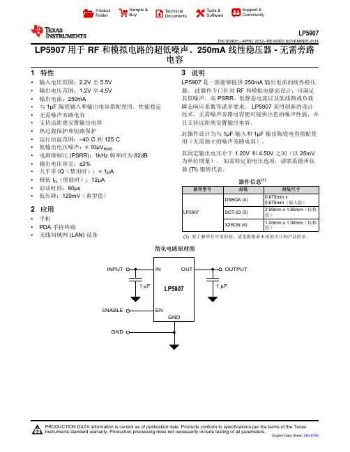
FINPUTENABLE GNDOUTPUTProduct FolderSample &BuyTechnical Documents Tools &SoftwareSupport &CommunityLP5907ZHCSD40H –APRIL 2012–REVISED NOVEMBER 2014LP5907用于RF 和模拟电路的超低噪声、250mA 线性稳压器-无需旁路电容1特性3说明•输入电压范围:2.2V 至5.5V LP5907是一款能够提供250mA 输出电流的线性稳压器。
此器件专门针对RF 和模拟电路而设计,可满足•输出电压范围:1.2V 至4.5V 其低噪声、高PSRR 、低静态电流以及低线路或负载•输出电流:250mA瞬态响应系数等诸多要求。
LP5907采用创新的设计•与1µF 陶瓷输入和输出电容搭配使用,性能稳定技术,无需噪声旁路电容便可提供出色的噪声性能,并•无需噪声旁路电容且支持远距离安置输出电容。
•支持远距离安置输出电容•热过载保护和短路保护此器件设计为与1µF 输入和1µF 输出陶瓷电容搭配使•运行结温范围:–40°C 到125C 用(无需独立的噪声旁路电容)。
•低输出电压噪声:<10µV RMS其固定输出电压介于1.20V 和4.50V 之间(以25mV •电源抑制比(PSRR):1kHz 频率时为82dB 为单位增量)。
如需特定的电压选项,请联系德州仪•输出电压容差:±2%器(TI)销售代表。
•几乎零IQ (禁用时):<1µA •极低I Q (使能时):12µA 器件信息(1)•启动时间:80µs器件型号封装封装尺寸•低压降:120mV (典型值)0.675mm xDSBGA (4)0.675mm (最大值)2.90mm x 1.60mm (标称2应用LP5907SOT-23(5)值)•手机1.00mm x 1.00mm (标称X2SON (4)•PDA 手持终端值)•无线局域网(LAN)设备(1)要了解所有可用封装,请见数据表末尾的可订购产品附录。
ABAQUS_疲劳分析简介

Low-cycle Fatigue in Bulk Materials
• Results
Damage initiation at joint toe Cycle number 199
Damage evolution Cycle number 749
Damage evolution Cycle number 801
Low-cycle Fatigue at Material Interfaces
• The onset and fatigue delamination growth at the interfaces are characterized by using the Paris Law, which relates crack growth rates da/dN to the relative fracture energy release rate G,
• The details of choosing characteristic length will be discussed later.
• Note: c3 depends on the system of units in which you are working; care is required to modify c3 when converting to a different system units.
CYCLEINI Number of cycles to initialized the damage
Low-cycle Fatigue in Bulk Materials
• Damage evolution for ductile damage in low-cycle fatigue • Once the damage initiation criterion is satisfied at a material point, the damage state is calculated and updated based on the inelastic hysteresis energy for the stabilized cycle. • The rate of the damage (dD/dN) at a material point per cycle is given by
双馈风电变流器IGBT模块损耗及结温的计算分析及变化规律研究

双馈风电变流器IGBT模块损耗及结温的计算分析及变化规律研究王臻卓;王慧;郝春玲【摘要】Aiming at the problem of the high failure rate caused by the IGBT module of the converter of double fed wind turbine generator,a calculation model under different working conditions of IGBT junction temperature and effect analyses were investigated.Firstly,a calculation model based on the switching period of machine side and grid side converter IGBT module was presented.Secondly,the effects of the IGBT steady state junction temperature were analyzed under conditions of different wind speed.Results showed that,with increasing wind speed,the overall loss of machine side and grid side converter IGBT module showed increasing trend,the change trend of the two parts was different in the local area.The temperature change of the IGBT module of the machine side converter is more severe than that of the net side.%针对双馈风电机组变流器由于IGBT模块失效造成高故障率的问题,提出了在不同工况下其 IGBT模块结温的准确计算方法及其变化规律分析.首先,建立了机侧及网侧变流器IGBT模块基于开关周期的损耗及结温计算模型;其次,在全工况运行下对机侧及网侧变流器IGBT模块损耗和稳态结温的变化规律进行了分析.结果表明,随着风速的不断增加,机侧及网侧变流器IGBT模块的损耗总体呈增大趋势,二者变化趋势局部不同;机侧变流器IGBT模块结温变化要比网侧的更为剧烈.【期刊名称】《电子器件》【年(卷),期】2017(040)002【总页数】5页(P296-300)【关键词】双馈风电变流器;IGBT;模块损耗;计算分析;变化规律【作者】王臻卓;王慧;郝春玲【作者单位】河南工业职业技术学院教务处,河南南阳 473000;河南工业职业技术学院机电自动化学院,河南南阳 473000;渤海船舶职业学院机电工程系,辽宁葫芦岛 125100【正文语种】中文【中图分类】TM464;TN32近年来,风力发电飞速发展,风机容量也随之不断上升,对电网的影响也越来越大。
Photovoltaic (pv) grid system

Abstract--This paper focuses on the study of a two-stage, multi-string photovoltaic (PV) system connected by a common DC bus to a centralized inverter, interfaced with a utility grid. The distribution network model, load model and DC bus model are used for simulation. PV system exhibits non-linear v-i characteristics and an intermediate boost converter is employed to operate the PV array at its maximum power point. An incremental conductance algorithm is employed to control the boost converter. A centralized inverter is controlled via a decoupled current control method and interfaced to the utility grid through a distribution transformer. The control of inverter is completely independent of maximum power point control of boost converter. Finally system stability is assessed with respect to variation in solar radiation of the PV and distribution network parameters.Index Terms--Photovoltaic, multi-string, two-stage, voltage-source converter, MPPT.I. N OMENCLATUREV s Inverter-filtered voltage; PCC voltageV l Load voltageV g Substation (grid) bus voltageV dc DC-link voltagei Inverter currenti g1Distribution line current between PCC and loadi g2Distribution line current between load and gridi l Load currenti pv PV module currentV pv PV module voltageP Real power output of PV system at PCCQ Reactive power output of PV system at PCCN Interface transformer turns ratioL Inductance of interface reactorR Resistance of interface reactorC f Shunt capacitance at PCCR1Line resistance between PCC and loadL1Line inductance between PCC and loadR2Line resistance between load and gridL2Line inductance between load and gridThis work was supported in part by the Florida Energy System Consortium under Grant HB7135.The authors are with Centre for Advanced Power Systems, Florida State University, Tallahassee, FL 32310 USA (e-mail: edrington; sarithab; {@}, jc09u@).C l Power factor correction capacitor at loadC dc DC link capacitanceR dc DC bus resistanceL dc DC bus inductanceω dq-frame angular speedρ dq-frame reference angleII. I NTRODUCTIONENEWABLE energy sources like solar, wind, biomassand fuel cells are good alternatives for conventionalpower generation. In recent years, due to the reduction incost of photovoltaic (PV) arrays, penetration of mediumpower PV systems into utility grid is becoming morecommon. The voltage rating up to 30 kV and power in therange of 10-100 MVA are classified as medium power withreference to AC side. The commercial scale PV panels of25MW capacity are planned for installation in Florida.SunPower Corporation has installed more than 400 MW of large-scale solar power systems around the world [1]. The perfor mance analysis of PV system is essential in order to ensure the reliability of grid. PV systems can be connected tothe grid using single-stage or two-stage topologies. A two-stage multi-string converter configuration, where one or morestrings of PV cells are connected to a single inverter, as in Fig.1, is more suitable for medium power applications [2].Fig. 1. Multi-string converter configurationThe maximum power point tracking (MPPT) technique can be implemented in DC/DC converters to achieve maximum efficiency of PV systems. Among the available DC/DCAnalysis and Control of a Multi-stringPhotovoltaic (PV) System Interfaced with aUtility GridChris S. Edrington, Senior Member, IEEE, Saritha Balathandayuthapani, Member, IEEE, and Jianwu CaoR978-1-4244-6551-4/10/$26.00 ©2010 IEEEconverters, buck and boost converters have a higher efficiency for a given cost [2]. Boost converters show significant advantages over buck converters, due to the presence of blocking diodes that prevent reverse flow of current into thePV cell [3]. The Incremental conductance (IncCond) methodis used for controlling the boost converter. The IncCondtechnique [4] can be implemented utilizing a DSP, which can easily keep track of previous values of current and voltages and make all the switching decisions. The current control of the inverter is implemented in the synchronous reference frame which yields a fast dynamic response and eliminates steady state error in three-phase inverter current. The decoupled current control and MPPT control were implemented in [5]; however, the distribution network model and DC bus model were not taken into account. Moreover, a detailed analysis of multi-string PV systems has yet to be accomplished.Many previous works deal with the penetration of PV systems into grid. In [6] the authors have conducted studies on single-phase two-stage PV systems with DC bus models. Isolated DC/DC converters in a single-phase two-stage PV system with emphasis on Eigen value analysis is given in [7]. The use of multiple PV systems with a boost converter andinverter connected to each module is illustrated in [8]. The common AC bus interconnecting the PV inverters is connected to the grid through an interfacing reactor. However, the distribution network and load model were not used in the analysis in [7-8]. Reference [9] has a detailed analysis of a single-stage PV system connected to the utility grid, using a distribution network and load model for stability analysis of the system. It is noted that, multi-string PV system with a centralized inverter and DC bus model were not used for any of the referenced studies.In this paper, the simulation of two-stage multi-string PV system connected by a common dc bus to a centralized inverter, interfaced with the utility grid are presented. Thedistribution network model, load model, DC bus model areused for simulation. Maximum power point control isimplemented in boost converter and decoupled current control is implemented in voltage source inverter (VSI). The rest of the paper is organized as follows- The system description is given in section III, the control of DC/DC converter and VSI are discussed in section IV and V, the small signal analysis is discussed in section VI, the simulation results are discussed in section VII, followed by conclusion in section VIII. III. D ESCRIPTION OF THE SYSTEMFig. 2 demonstrates the one-line diagram of a multi-string PV system connected to the grid. Each PV module consists of 176 parallel and 150 series arrays. The output of the PV is highly non-linear and thus can not be represented by a simple current or voltage source in parallel with the diode. The model of a PV module is built using PLECS library components [10] as shown in Fig. 3. The output voltage of the PV module, V PV , is a function of solar radiation and environmental temperature. The voltage V PV is fed to the inverter through a dc transmission line. The dc line is considered to be a short transmission line and represented by RL equivalent circuit. The boost converters are assumed to be at an equal distance from the centralized inverter. The capacitor C dc is a dc link capacitor at the input of the inverter. The output of inverter is connected to the distribution network through an interfacing reactor at the pointof common coupling (PCC). The filter capacitor C f provides the low-impedance path for the current harmonics generated by inverter.The distribution network consists of a transformer T r1, loadand capacitor C l . The capacitor C l is used for load powerfactor correction. The low voltage side of T r1 is deltaconnected to the PV inverter and its high voltage side has agrounded wye connection. The transmission line between load and PCC is represented by R 1 and L 1. The distribution network is connected to the grid V gthrough a transmissionline represented by R 2 and L 2, assuming a short line approximation.Fig. 2. Single-line schematic diagram of multi-string PV system interfaced to a utility gridFig. 3. Circuit representation of a PV moduleIV. C ONTROL OF BOOST CONVERTERHigh initial cost and limited life span of PV arrays make it more important to extract as much power from them aspossible. Several MPPT algorithms have been proposed in literature with the IncCond method [11] being one of the morepopular among them. PV arrays must be operated at a V ref PV , where maximum power can be extracted from the PV. TheIncCond control strategy is based on the fact that the slope of the PV array power curve is zero at the maximum power point(MPP), positive on the left and negative on the right of MPP. By comparing the instantaneous conductance (i/v) to the incremental conductance (Δi/Δv), the reference voltage V ref PV is adjusted. At the MPP, V ref PV is equal to V MPP PV . Once the MPP is reached, the operation of the PV array is maintained at V MPPPV unless there is a change in ΔI, in which the algorithm decrements or increments V ref PV to track the new MPP. Theincrement size determines how fast the MPP is tracked. Fig. 4. Control circuit of boost converterIn a boost converter, the input capacitor voltage is compared with the V ref PV , which is obtained from the IncCond algorithm. When the capacitor voltage exceeds V ref PV , the switch is turned ON and capacitor is discharged. When the capacitor voltage reduces below a lower limit, the switch is turned off. The desired switching frequency of the boost converter f d is selected as 20KHz. The lower limit is a function of switching frequency and current i pv . There is a trade-off between switching frequency and capacitor value C 1 to get the desired voltage variation. This control structure is implemented in [12] to control the buck converter of a current source inverter. In this paper, the same control strategy as shown in Fig. 4 is used to control the boost converter feeding the voltage source inverter.V. C ONTROL OF VOLTAGE SOURCE INVERTERThe real power output of inverter is regulated by controlling i d and the reactive power is regulated by controlling i q . The voltage V PV and I PV of PV module is usedfor calculating the real power output of the inverter, pumpedinto distribution network. ...2211++=PV PV PV PV ref I V I V P(1) The reactive power Q ref injected into the network from theinverter is set to zero. When the output voltage and power references are known, the current reference can be calculated via a power calculator. The references are calculated according to⎥⎦⎤⎢⎣⎡⎥⎦⎤⎢⎣⎡−+∗=⎥⎦⎤⎢⎣⎡ref ref sd sq sq sd q d qref dref Q P V V V V V V I I 22132 (2) The error signal e d = i dref - i d and e q =i qref -i qare passed througha PI controller. The PI controller constants are chosen such thati i i p RK L K ττ==(3) W here τi is time constant of current control loop. The switching frequency of inverter is 3 kHz and the time constantτi is taken as ten times smaller than the switching time [9]. It should be made small for a fast current-control response, but adequately large so that the bandwidth of the closed-current loop is smaller than the switching frequency.Fig. 5. a) Switch model in PSCAD b) Linear model in MATLABVI. S MALL SIGNAL ANALYSISThe linear model of the system is built in Matlab for stability analysis. The overall system is given byU B X A X sys sys +=* (4) The linear model is the function of steady state operating pointof PV system. Eigen values lie in left hand side of the S-plane and the system is stable. The model is validated by comparingthe results with switching model in PSCAD. The solar radiation in PV2 is varied from S=1 to 0.5 at t=0.7s. The change in interface current is compared in Fig. 5. The steady state values of current are equal but the transients differ asdynamics of boost converter is not considered in linear model.In future studies, we plan to include the dynamics of Boostconverter in our study. VII. S IMULATION RESULTSSimulation of the model given in Fig. 2 has been accomplished using Simulink and PLECS. The parameters of the system are given in Table I.A. Solar irradiation S=1 in PV1 and PV2The diode rectifier, induction motor and RL load are connected to the distribution network. The size of the loads is available in Table I. Both the PV modules have solar radiation S=1 i.e. 1000 w/m 2 and plot of dq axes inverter currents are shown in Fig. 6. The dc voltage of the inverter V dc is shown in Fig. 7. The PCC current and voltage are shown in Fig. 8.Time (Sec)C u r r e n t (A )Fig. 6. I d and I q of PV inverter with S=1 in both PV modulesTime (sec)V o l t a g e (V )Fig. 7. V dc of PV inverter with S=1 in both PV modulesB. Change in Solar irradiation of PV2A disturbance in the system is caused by changing the solar irradiation of the 2nd PV module from S = 1 to S = 0.2 at t = 0.4s. As can be seen, there is a change in the operating point of PV2 and the inverter current is varied accordingly as shownin Fig. 9. The voltage V dc of the inverter changes, as in Fig. 10.TABLE I S YSTEM PARAMETERST r1 nominal Power 3.5 MVAT r1 Voltage Ratio 6.6/0.48 KV T r1 leakage inductance 0.1 pu T r1 Resistance 0.02 pu Interface resistance 3e-3 Ω Interface inductance 250e-3 H Filter capacitance600e-6 F Switching frequency of inverter 3e3 HzDC bus resistance 3e-3 Ω per unit length DC bus inductance50e-6 H per unit length Length of Common DC bus to inverter 10 units Length of DC bus from Boost converter to Common DC point 2 units Grid voltage 6.6 KV rmsLine inductance 0.105e-3 H per unit length Line resistance5e-3 Ω per unit length Length of Transmission line 20 units R-L Load Parameter Resistance Inductance50 Ω 10e-3 H Diode Rectifier Load Resistance Load inductance100 Ω 10e-3 H Induction Motor Stator resistance Stator inductance Rotor resistance Rotor inductanceMagnetizing inductance Inertia0.8 4e-3 0.8 2e-3 70e-3 0.1Time (Sec)V o l t a g e (V ),C u r r e n t (A )Fig. 8. PCC current and voltage with S=1 in both PV modulesC. Fault at PV2When a PV module develops a fault, it is isolated by virtue of, from the boost converter. This is simulated in the 2nd PV module at t = 0.4s and it is shown that the system will remain stable with only PV1 energizing the inverter. The change in inverter current is shown in Fig. 11.Time (sec)C u r r e n t (A )Fig. 9. I d of PV inverter under change in solar radiationTime (sec)V o l t a g e (V )Fig. 10. V dc of PV inverter under change in solar radiationTime (sec)C u r r e n t (A )Fig. 11. I d current of PV inverter with PV2 openD. Change in load connected to the gridThe RL load is connected to the grid and a diode rectifier is introduced into the distribution network at t = 0.35 s. The PVmodules are operating at their MPP and the introduction of non-linear load affects the harmonic content of the inverter current. Fig. 12 shows the increase in RMS value of grid current, to supply the power required by the non-linear load and inverter output current. When an induction motor is line started at t = 0.3s, there is a high inrush current in the network. It is reflected as transients in the inverter current, as seen in Fig. 13.E. Drop in grid voltageWith the diode rectifier and RL load connected into the network, there is a drop in grid voltage by 20% at t = 0.35s and the voltage restores its level after 200ms. In [7], when the voltage drops for a longer duration (200ms), the PV system collapses. In our model, the PV system is stable and it is able to restore its original value as seen in Fig. 14. The PV system is stable due to decoupled current control algorithm.F. Fault at DC BusWhen the RL load is connected into the network, there is a fault at DC bus close to the voltage source inverter at t=0.5s. The dc voltage drops to zero and the transients in interface current is shown in Fig. 15. The circuit breaker opens at t=0.6s. The fault is cleared at t=0.75s and the breaker recloses at t=0.8s. The system attains its pre-fault condition without error.Time (sec)C u r r e n t (A )Time (sec)C u r r e n t (A )Fig. 12. I d of PV inverter and grid current with non-linear load in the networkTime (sec)C u r r e n t (A )Fig. 13. I d of PV inverter with line-start induction motor in the networkTime (sec)C u r r e n t (A )Time (sec)V o l a t g e (V )Fig. 14. I d and V d of PV inverter with drop in grid voltage and fault cleared after 200 msTime (Sec)C u r r e n t (A )Fig. 15. I d at PCC with fault at DC bus at t=0.5s and fault cleared after250 msVIII. C ONCLUSION A Multi-string PV system is interfaced into a distribution network and has been investigated. The MPPT control of DC/DC converter and decoupled current control of inverter are employed in the system. The transient response of the system has been studied under disturbance conditions and abasic analysis has been conducted. It can be concluded fromthe simulated results that the combined PV–utility system is stable under different disturbance conditions and that performance is acceptable.IX. R EFERENCES[1] Mike R. Lopez, “Florida power & light breaks ground for biggest solar photovoltaic installation in the US”, , para. 1, March 03,2009. [Online]. Available: /en/general-green-news/green-business-news/corporate-communications/846. [Accessed:Feb. 05, 2010].[2]G. Walker and P. Sernia, “Cascaded DC/DC converter connection ofphotovoltaic modules”, IEEE Trans. Power Electronics , vol. 19, pp.1130-1139, Jul. 2004.[3] Weidong Xiao, Nathan Ozog, and William G. Dunford, “Topology studyof photovoltaic Interface for maximum power point tracking”, IEEE Trans. Ind. Electronics , vol. 54, pp. 1696-1704, Jun. 2007.[4] W. Wu, N. Pongratanankul, W. Qiu, K. Rustom, T. Kasparis, and I.Bataresh, “DSP-based multiple peak power tracking for expandable power system” in 18th Ann. IEEE Appl. Power Electronic Conf. and Expo ., 2003, pp. 525-530.[5] M. Milosevic, G.Anderson, and S. Garbic, “Decoupling current controland maximum power point control in small power network with Photovoltaic Source” in Power Systems Conf. and Expo. 2006, pp. 1005-1011.[6] Li Wang, and Ying-Hao Lin, “Dynamic stability of a photovoltaic arrayconnected to a large utility grid”, in Proc. IEEE Power Eng. Soc. Winter Meeting , 2000, vol. 1, pp. 476-480.[7] C. Rodriguez, and G.A.J. Amaratunga, “Dynamic stability of a gridconnected photovoltaic systems”, in Proc. IEEE Power Eng. Soc. General Meeting , 2004, vol. 2, pp. 2193-2199.[8] Li Wang, and Tzu-Ching Lin, “Dynamic stability and transient responseof multiple grid-connected PV systems”, in Transmission and Distribution Conf. and Expo . 2008, pp. 1-6.[9] A. Yazdani, and P. P. Dash, “A control methodology andcharacterization of dynamics for a photovoltaic system interfaced with a distribution network”, IEEE Trans. Power Delivery , vol. 24, pp. 1538-1551, Jul. 2009.[10] Ryan C. Campbell, “A circuit-based photovoltaic array model for powersystem studies”, in 39th North American Power Symposium , 2007, pp. 97-101.[11] S. Jain, and V. Agarwal, “Comparison of the performance of maximumpower point tracking schemes as applied to single-stage grid connected photovoltaic systems”, IET Electric Power Applications , vol. 1, pp. 753-762, Sept. 2007.[12] S.A. Khajehoddin, A. Bakhshai, and P. Jain, “A novel toplogy andcontrol strategy for maximum power point trackers and multi-string grid-connected PV interface”, in 23rd Annu. IEEE Applied Power Elec. Conf. and Expo . 2008, pp. 173-178.X. B IOGRAPHIESChris S. Edrington (S’94, M’04, SM’09) received his Ph.D. in electrical engineering from theUniversity of Missouri-Rolla in 2004 where he wasboth a GAANN and IGERT fellow. From 2004 ~ 2007, he was an Assistant Professor of Electrical Engineering in the College of Engineering at Arkansas State University. He currently is an Assistant Professor of Electrical and Computer Engineering with the FAMU-FSU College ofEngineering and is a research associate for theFlorida State University-Center for Advanced Power Systems. His research interests include modeling, simulation, and control of electromechanical drivesystems; applied power electronics; and integration of distributed energyresources.Saritha Balathandayuthapani (S’01, M’03, SM’07) received the Ph.D. degree in electricalengineering from Indian Institute of Technology,Madras, India in 2007. She was with GE Global research, India. She joined CAPS, Florida StateUniversity, FL, USA in 2009, where she is currently pursuing Post-doc. Her research interests include control of power electronic converters, renewableenergy, machines and drives.Jianwu Cao (S’09) received the B.Eng degree in Electrical Engineering from Huazhong University of Science and Technology, Wuhan, China, in 2009. He joined the Center for Advanced Power Systems, Florida State University, Tallahassee, FL, in 2009, where he is currently pursing his Ph.D. degree. His research interests include distributed generation, renewable energy, and power system.。
- 1、下载文档前请自行甄别文档内容的完整性,平台不提供额外的编辑、内容补充、找答案等附加服务。
- 2、"仅部分预览"的文档,不可在线预览部分如存在完整性等问题,可反馈申请退款(可完整预览的文档不适用该条件!)。
- 3、如文档侵犯您的权益,请联系客服反馈,我们会尽快为您处理(人工客服工作时间:9:00-18:30)。
failures of the affected components but results in an increase or decrease of deterioration of the affected components. In Type 1 failure dependence (IFD), when a component fails, it will either cause the affected components to fail with probability p or leave no effect on the affected components with probability 1- p. Further discussion on IFD can be found in [2]-[4]. Type 2 s-dependence implies that the failure of a component affects the failure rates of the affected components. Sun et al. [1] modeled the failure rate of an affected component by adding a portion of failure rate from the influencing component to its independent failure rate. Lai and Chen [5] studied a two-unit system with Type 2 failure dependence. The failure of unit 1 causes damage to unit 2 by increasing the failure rate of unit 2 by a certain amount corresponding to the number of failures experienced by unit 1. Rasmekonen and Parlikad [6] considered a system consisting of M parallel non-critical machines feeding a critical machine. Parallel elements are independent but the performance of the critical component decreases when a non-critical component fails. The failure and repair times of components were assumed to be deterministic. In practice, many systems and components can degrade and operate at reduced performance levels. As a component deteriorates, its performance may be in several states varying from perfect functioning to complete failure. Such a component is called multi-state component, and a system consisting of multi-state components is called multi-state system (MSS). MSS with s-independent components have been studied in the literature. General concepts and reliability analysis methods can be found in [7]. Recently, more efforts have been made on the analysis of MSS with dependent components. Levitin [8] studied the reliability evaluation problem for MSS with dependent components using the universal generating function (UGF) technique. He assumed that the conditional probability distributions of the affected components are deterministic and explicitly known. In addition, the detailed mechanism of s-dependence was not discussed. Type 1 s-dependence in multi-state systems can be treated in the same way as in binary systems, i.e. the failure of a
Reliability Analysis of Multi-state Systems with S-dependent Components
Cuong D. Dao, University of Alberta Ming J. Zuo, PhD, University of Alberta
Key Words: Multi-state systems, multi-state components, s-dependence, reliability, universal generating function, Monte Carlo simulation SUMMARY & CONCLUSIONS The assumption of stochastic independence between components is frequently made in studies of system reliability. However, in a specific system, the failure of a component can trigger the failure of other components, or the current health condition of a component may affect the performance of other components. Thus, the state of a component can affect the state and degradation of other components in a multicomponent system, that is, stochastic dependence (sdependence) may exist in real and complex systems. In this paper, reliability analysis of multi-state systems (MSS) with sdependent components will be considered. The MSS consists of 2 multi-state components in series, with each component possibly operating at different performance levels, varying from perfect functioning to complete failure. When the first component degrades to a lower performance level, it affects the state as well as the degradation of the other component in the system. A combined technique of stochastic process and modified universal generating function is used to evaluate the system reliability. The combined approach is then verified using the Monte Carlo Simulation method. An illustrative example on reliability analysis of MSS with dependent components is also provided. 1 INTRODUCTION In binary systems, s-dependence is referred to as “failure dependence” and it is often analyzed based on the nature of components’ failures or operating modes. The components are interconnected in a specific system design or subjected to a common stress such as operating environment, shocks, etc. Thus, the failure of a component may affect the operation of other components in a multi-component system. In [1], sdependence between components is referred to as “interactive failure” and it can be categorized into two types based on the consequences that arise when a component in the system fails. • Type 1 - Immediate failure dependence (IFD): whenonent) fails, it immediately causes the failures of other components (affected components). • Type 2 - Gradual degradation dependence: The failure of the influencing component does not immediately cause