turbulence modeling options in fluent
fluent二维大涡模拟命令
fluent二维大涡模拟命令Fluent是流体动力学模拟软件的一种,它提供了二维大涡模拟命令用于模拟二维涡旋动力学过程。
本文将分步骤阐述如何使用Fluent二维大涡模拟命令。
第一步,打开Fluent软件。
进入“File”菜单,选择“New”打开一个新的工作文件。
在Fluent主界面的左侧面板选择“2D”选项卡,然后选择“Viscous”和“Steady”选项后点击“Create/Edit”按钮。
第二步,进入“Grid”界面。
在“Mesh”选项卡中选择“2D Mesh”菜单,选择“Triangle”网格类型。
随后,选择“Mechanical”类型并调整所需参数,包括网格的大小、分辨率、以及其他关键点的划分数量。
最后,点击“Generate Mesh”按钮生成网格。
第三步,设置边界条件。
在Fluent主界面的左侧面板选择“Boundary Conditions”选项卡。
根据需要设置边界条件,包括入口和出口边界、容器壁边界和物体边界。
基本的物理条件包括质量流速、温度和密度。
第四步,设置模拟参数。
在Fluent主界面的左侧面板选择“Solution”选项卡。
首先选择“Viscous”和“Steady”选项,然后在“Methods”菜单中选择“Unsteady”. 调整所需参数并计算时间,包括时间步长和计算时间范围。
第五步,开始求解二维大涡模拟。
在Fluent主界面的左侧面板选择“Compute”选项卡,点击“Start Calculation”按钮开始求解。
第六步,查看二维大涡模拟结果。
在Fluent主界面的左侧面板选择“Graphics”选项卡。
根据需要选择显示不同的结果,包括速度分布、温度变化、实体形态等等。
以上是使用Fluent二维大涡模拟命令的步骤。
通过学习和实践,我们可以使用Fluent来分析和解决各种相关的物理、化学和工程问题。
fluent中多孔介质设置问题和算例

经过痛苦的一段经历,终于将局部问题真相大白,为了使保位某某不再经过我之痛苦,现在将本人多孔介质经验公布如下,希望各位能加精:1。
Gambit中划分网格之后,定义需要做为多孔介质的区域为fluid,与缺省的fluid分别开来,再定义其名称,我习惯将名称定义为porous;2。
在fluent中定义边界条件define-boundary condition-porous(刚定义的名称),将其设置边界条件为fluid,点击set按钮即弹出与fluid边界条件一样的对话框,选中porous zone与laminar复选框,再点击porous zone标签即出现一个带有滚动条的界面;3。
porous zone设置方法:1〕定义矢量:二维定义一个矢量,第二个矢量方向不用定义,是与第一个矢量方向正交的;三维定义二个矢量,第三个矢量方向不用定义,是与第一、二个矢量方向正交的;〔如何知道矢量的方向:打开grid图,看看X,Y,Z的方向,如果是X向,矢量为1,0,0,同理Y向为0,1,0,Z向为0,0,1,如果所需要的方向与坐标轴正向相反,如此定义矢量为负〕圆锥坐标与球坐标请参考fluent帮助。
2〕定义粘性阻力1/a与内部阻力C2:请参看本人上一篇博文“终于搞清fluent中多孔粘性阻力与内部阻力的计算方法〞,此处不赘述;3〕如果了定义粘性阻力1/a与内部阻力C2,就不用定义C1与C0,因为这是两种不同的定义方法,C1与C0只在幂率模型中出现,该处保持默认就行了;4〕定义孔隙率porousity,默认值1表示全开放,此值按实验测值填写即可。
完了,其他设置与普通k-e或RSM一样。
总结一下,与君共享!Tutorial 7. Modeling Flow Through Porous MediaIntroductionMany industrial applications involve the modeling of flow through porous media, such as filters, catalyst beds, and packing. This tutorial illustrates how to set up and solve a problem involving gas flow through porous media.The industrial problem solved here involves gas flow through a catalytic converter. Catalytic converters are monly used to purify emissions from gasoline and diesel engines by converting environmentally hazardous exhaust emissions to acceptable substances.Examples of such emissions include carbon monoxide (CO), nitrogen oxides (NOx), and unburned hydrocarbon fuels. These exhaust gas emissions are forced through a substrate, which is a ceramic structure coated with a metal catalyst such as platinum or palladium.The nature of the exhaust gas flow is a very important factor in determining the performance of the catalytic converter. Of particular importance is the pressure gradient and velocity distribution through the substrate. Hence CFD analysis is used to design efficient catalytic converters: by modeling the exhaust gas flow, the pressure drop and the uniformity of flow through the substrate can be determined. In this tutorial, FLUENT is used to model the flow of nitrogen gas through a catalytic converter geometry, so that the flow field structure may be analyzed.This tutorial demonstrates how to do the following:_ Set up a porous zone for the substrate with appropriate resistances._ Calculate a solution for gas flow through the catalytic converter using the pressure based solver. _ Plot pressure and velocity distribution on specified planes of the geometry._ Determine the pressure drop through the substrate and the degree of non-uniformity of flow through cross sections of the geometry using X-Y plots and numerical reports.Problem DescriptionThe catalytic converter modeled here is shown in Figure 7.1. The nitrogen flows in through the inlet with a uniform velocity of 22.6 m/s, passes through a ceramic monolith substrate with square shaped channels, and then exits through the outlet.While the flow in the inlet and outlet sections is turbulent, the flow through the substrate is laminar and is characterized by inertial and viscous loss coefficients in the flow (X) direction. The substrate is impermeable in other directions, which is modeled using loss coefficients whose values are three orders of magnitude higher than in the X direction.Setup and SolutionStep 1: Grid1. Read the mesh file (catalytic converter.msh).File /Read /Case...2. Check the grid. Grid /CheckFLUENT will perform various checks on the mesh and report the progress in the console. Make sure that the minimum volume reported is a positive number.3. Scale the grid.Grid! Scale...(a) Select mm from the Grid Was Created In drop-down list.(b) Click the Change Length Units button. All dimensions will now be shown in millimeters.(c) Click Scale and close the Scale Grid panel.4. Display the mesh. Display /Grid...(a) Make sure that inlet, outlet, substrate-wall, and wall are selected in the Surfaces selection list.(b) Click Display.(c) Rotate the view and zoom in to get the display shown in Figure 7.2.(d) Close the Grid Display panel.The hex mesh on the geometry contains a total of 34,580 cells.Step 2: Models1. Retain the default solver settings. Define /Models /Solver...2. Select the standard k-ε turbulence model. Define/ Models /Viscous...Step 3: Materials1. Add nitrogen to the list of fluid materials by copying it from the Fluent Database for materials.Define /Materials...(a) Click the Fluent Database... button to open the Fluent Database Materials panel.i. Select nitrogen (n2) from the list of Fluent Fluid Materials.ii. Click Copy to copy the information for nitrogen to your list of fluid materials. iii. Close the Fluent Database Materials panel.(b) Close the Materials panel.Step 4: Boundary Conditions. Define /Boundary Conditions...1. Set the boundary conditions for the fluid (fluid).(a) Select nitrogen from the Material Name drop-down list.(b) Click OK to close the Fluid panel.2. Set the boundary conditions for the substrate (substrate).(a) Select nitrogen from the Material Name drop-down list.(b) Enable the Porous Zone option to activate the porous zone model.(c) Enable the Laminar Zone option to solve the flow in the porous zone without turbulence.(d) Click the Porous Zone tab.i. Make sure that the principal direction vectors are set as shown in Table7.1. Use the scroll bar to access the fields that are not initially visible in the panel.ii. Enter the values in Table 7.2 for the Viscous Resistance and Inertial Resistance. Scroll down to access the fields that are not initially visible in the panel.(e) Click OK to close the Fluid panel.3. Set the velocity and turbulence boundary conditions at the inlet (inlet).(a) Enter 22.6 m/s for the Velocity Magnitude.(b) Select Intensity and Hydraulic Diameter from the Specification Method dropdown list in the Turbulence group box.(c) Retain the default value of 10% for the Turbulent Intensity.(d) Enter 42 mm for the Hydraulic Diameter.(e) Click OK to close the Velocity Inlet panel.4. Set the boundary conditions at the outlet (outlet).(a) Retain the default setting of 0 for Gauge Pressure.(b) Select Intensity and Hydraulic Diameter from the Specification Method dropdown list in the Turbulence group box.(c) Enter 5% for the Backflow Turbulent Intensity.(d) Enter 42 mm for the Backflow Hydraulic Diameter.(e) Click OK to close the Pressure Outlet panel.5. Retain the default boundary conditions for the walls (substrate-wall and wall) and close the Boundary Conditions panel.Step 5: Solution1. Set the solution parameters. Solve /Controls /Solution...(a) Retain the default settings for Under-Relaxation Factors.(b) Select Second Order Upwind from the Momentum drop-down list in the Discretization group box.(c) Click OK to close the Solution Controls panel.2. Enable the plotting of residuals during the calculation. Solve/Monitors /Residual...(a) Enable Plot in the Options group box.(b) Click OK to close the Residual Monitors panel.3. Enable the plotting of the mass flow rate at the outlet.Solve / Monitors /Surface...(a) Set the Surface Monitors to 1.(b) Enable the Plot and Write options for monitor-1, and click the Define... button to open the Define Surface Monitor panel.i. Select Mass Flow Rate from the Report Type drop-down list.ii. Select outlet from the Surfaces selection list.iii. Click OK to close the Define Surface Monitors panel.(c) Click OK to close the Surface Monitors panel.4. Initialize the solution from the inlet. Solve /Initialize /Initialize...(a) Select inlet from the pute From drop-down list.(b) Click Init and close the Solution Initialization panel.5. Save the case file (catalytic converter.cas). File /Write /Case...6. Run the calculation by requesting 100 iterations. Solve /Iterate...(a) Enter 100 for the Number of Iterations.(b) Click Iterate.The FLUENT calculation will converge in approximately 70 iterations. By this point the mass flow rate monitor has attended out, as seen in Figure 7.3.(c) Close the Iterate panel.7. Save the case and data files (catalytic converter.cas and catalytic converter.dat).File /Write /Case & Data...Note: If you choose a file name that already exists in the current folder, FLUENTwill prompt you for confirmation to overwrite the file.Step 6: Post-processing1. Create a surface passing through the centerline for post-processing purposes.Surface/Iso-Surface...(a) Select Grid... and Y-Coordinate from the Surface of Constant drop-down lists.(b) Click pute to calculate the Min and Max values.(c) Retain the default value of 0 for the Iso-Values.(d) Enter y=0 for the New Surface Name.(e) Click Create.2. Create cross-sectional surfaces at locations on either side of the substrate, as well as at its center.Surface /Iso-Surface...(a) Select Grid... and X-Coordinate from the Surface of Constant drop-down lists.(b) Click pute to calculate the Min and Max values.(c) Enter 95 for Iso-Values.(d) Enter x=95 for the New Surface Name.(e) Click Create.(f) In a similar manner, create surfaces named x=130 and x=165 with Iso-Values of 130 and 165, respectively. Close the Iso-Surface panel after all the surfaces have been created.3. Create a line surface for the centerline of the porous media.Surface /Line/Rake...(a) Enter the coordinates of the line under End Points, using the starting coordinate of (95, 0, 0) and an ending coordinate of (165, 0, 0), as shown.(b) Enter porous-cl for the New Surface Name.(c) Click Create to create the surface.(d) Close the Line/Rake Surface panel.4. Display the two wall zones (substrate-wall and wall). Display /Grid...(a) Disable the Edges option.(b) Enable the Faces option.(c) Deselect inlet and outlet in the list under Surfaces, and make sure that only substrate-wall and wall are selected.(d) Click Display and close the Grid Display panel.(e) Rotate the view and zoom so that the display is similar to Figure 7.2.5. Set the lighting for the display. Display /Options...(a) Enable the Lights On option in the Lighting Attributes group box.(b) Retain the default selection of Gourand in the Lighting drop-down list.(c) Click Apply and close the Display Options panel.6. Set the transparency parameter for the wall zones (substrate-wall and wall).Display/Scene...(a) Select substrate-wall and wall in the Names selection list.(b) Click the Display... button under Geometry Attributes to open the Display Properties panel.i. Set the Transparency slider to 70.ii. Click Apply and close the Display Properties panel.(c) Click Apply and then close the Scene Description panel.7. Display velocity vectors on the y=0 surface.Display /Vectors...(a) Enable the Draw Grid option. The Grid Display panel will open.i. Make sure that substrate-wall and wall are selected in the list under Surfaces.ii. Click Display and close the Display Grid panel.(b) Enter 5 for the Scale.(c) Set Skip to 1.(d) Select y=0 from the Surfaces selection list.(e) Click Display and close the Vectors panel.The flow pattern shows that the flow enters the catalytic converter as a jet, with recirculation on either side of the jet. As it passes through the porous substrate, it decelerates and straightens out, and exhibits a more uniform velocity distribution.This allows the metal catalyst present in the substrate to be more effective.Figure 7.4: Velocity Vectors on the y=0 Plane8. Display filled contours of static pressure on the y=0 plane.Display /Contours...(a) Enable the Filled option.(b) Enable the Draw Grid option to open the Display Grid panel.i. Make sure that substrate-wall and wall are selected in the list under Surfaces.ii. Click Display and close the Display Grid panel.(c) Make sure that Pressure... and Static Pressure are selected from the Contours of drop-down lists.(d) Select y=0 from the Surfaces selection list.(e) Click Display and close the Contours panel.Figure 7.5: Contours of the Static Pressure on the y=0 planeThe pressure changes rapidly in the middle section, where the fluid velocity changes as it passes through the porous substrate. The pressure drop can be high, due to the inertial and viscous resistance of the porous media. Determining this pressure drop is a goal of CFD analysis. In the next step, you will learn how to plot the pressure drop along the centerline of the substrate.9. Plot the static pressure across the line surface porous-cl.Plot /XY Plot...(a) Make sure that the Pressure... and Static Pressure are selected from the Y Axis Function drop-down lists.(b) Select porous-cl from the Surfaces selection list.(c) Click Plot and close the Solution XY Plot panel.Figure 7.6: Plot of the Static Pressure on the porous-cl Line SurfaceIn Figure 7.6, the pressure drop across the porous substrate can be seen to be roughly 300 Pa.10. Display filled contours of the velocity in the X direction on the x=95, x=130 and x=165 surfaces.Display /Contours...(a) Disable the Global Range option.(b) Select Velocity... and X Velocity from the Contours of drop-down lists.(c) Select x=130, x=165, and x=95 from the Surfaces selection list, and deselect y=0.(d) Click Display and close the Contours panel.The velocity profile bees more uniform as the fluid passes through the porous media. The velocity is very high at the center (the area in red) just before the nitrogen enters the substrate and then decreases as it passes through and exits the substrate. The area in green, which corresponds to a moderate velocity, increases in extent.Figure 7.7: Contours of the X Velocity on the x=95, x=130, and x=165 Surfaces11. Use numerical reports to determine the average, minimum, and maximum of the velocity distribution before and after the porous substrate.Report /Surface Integrals...(a) Select Mass-Weighted Average from the Report Type drop-down list.(b) Select Velocity and X Velocity from the Field Variable drop-down lists.(c) Select x=165 and x=95 from the Surfaces selection list.(d) Click pute.(e) Select Facet Minimum from the Report Type drop-down list and click pute again.(f) Select Facet Maximum from the Report Type drop-down list and click pute again.(g) Close the Surface Integrals panel.The numerical report of average, maximum and minimum velocity can be seen in the main FLUENT console, as shown in the following example:word21 /21The spread between the average, maximum, and minimum values for X velocity gives the degree to which the velocity distribution is non-uniform. You can also use these numbers to calculate the velocity ratio (i.e., the maximum velocity divided by the mean velocity) and the space velocity (i.e., the product of the mean velocity and the substrate length).Custom field functions and UDFs can be also used to calculate more plex measures of non-uniformity, such as the standard deviation and the gamma uniformity index.SummaryIn this tutorial, you learned how to set up and solve a problem involving gas flow through porous media in FLUENT. You also learned how to perform appropriate post-processing to investigate the flow field, determine the pressure drop across the porous media and non-uniformity of the velocity distribution as the fluid goes through the porous media.Further ImprovementsThis tutorial guides you through the steps to reach an initial solution. You may be able to obtain a more accurate solution by using an appropriate higher-order discretization scheme and by adapting the grid. Grid adaption can also ensure that the solution is independent of the grid. These steps are demonstrated in Tutorial 1.。
Fluent模型使用技巧
1.多相流动模式我们可以根据下面的原则对多相流分成四类:•气-液或者液-液两相流:o气泡流动:连续流体中的气泡或者液泡。
o液滴流动:连续气体中的离散流体液滴。
o活塞流动:在连续流体中的大的气泡o分层自由面流动:由明显的分界面隔开的非混合流体流动。
•气-固两相流:o充满粒子的流动:连续气体流动中有离散的固体粒子。
o气动输运:流动模式依赖诸如固体载荷、雷诺数和粒子属性等因素。
最典型的模式有沙子的流动,泥浆流,填充床,以及各向同性流。
o流化床:由一个盛有粒子的竖直圆筒构成,气体从一个分散器导入筒内。
从床底不断充入的气体使得颗粒得以悬浮。
改变气体的流量,就会有气泡不断的出现并穿过整个容器,从而使得颗粒在床内得到充分混合。
•液-固两相流o泥浆流:流体中的颗粒输运。
液-固两相流的基本特征不同于液体中固体颗粒的流动。
在泥浆流中,Stokes数通常小于1。
当Stokes数大于1时,流动成为流化(fluidization)了的液-固流动。
o水力运输:在连续流体中密布着固体颗粒o沉降运动:在有一定高度的成有液体的容器内,初始时刻均匀散布着颗粒物质。
随后,流体将会分层,在容器底部因为颗粒的不断沉降并堆积形成了淤积层,在顶部出现了澄清层,里面没有颗粒物质,在中间则是沉降层,那里的粒子仍然在沉降。
在澄清层和沉降层中间,是一个清晰可辨的交界面。
•三相流(上面各种情况的组合)各流动模式对应的例子如下:•气泡流例子:抽吸,通风,空气泵,气穴,蒸发,浮选,洗刷•液滴流例子:抽吸,喷雾,燃烧室,低温泵,干燥机,蒸发,气冷,刷洗•活塞流例子:管道或容器内有大尺度气泡的流动•分层自由面流动例子:分离器中的晃动,核反应装置中的沸腾和冷凝•粒子负载流动例子:旋风分离器,空气分类器,洗尘器,环境尘埃流动•风力输运例子:水泥、谷粒和金属粉末的输运•流化床例子:流化床反应器,循环流化床•泥浆流例子:泥浆输运,矿物处理•水力输运例子:矿物处理,生物医学及物理化学中的流体系统•沉降例子:矿物处理2.多相流模型FLUENT中描述两相流的两种方法:欧拉一欧拉法和欧拉一拉格朗日法,后面分别简称欧拉法和拉格朗日法。
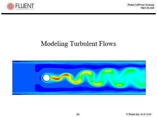
ansys fluent教程fluent12-lecture06-turbulence

Flux of energy
Dissipating eddies
Energy Cascade (after Richardson, 1922)
ANSYS, Inc. Proprietary © 2009 ANSYS, Inc. All rights reserved.
6-4
April 28, 2009 Inventory #002600
Turbulence Modeling
Introduction to Turbulence Modeling
Training Manual
• Characterization of Turbulent Flows • From Navier-Stokes Equations to Reynolds-Averaged Navier-Stokes (RANS) Models • Reynolds Stress Tensor and the Closure Problem • Turbulence Kinetic Energy (k) Equation • Eddy Viscosity Models (EVM) • Reynolds Stress Model • Near-wall Treatments Options and Mesh Requirement • Inlet Boundary Conditions • Summary: Turbulence Modeling Guidelines • Appendix
• Very sensitive to (or dependent on) initial conditions.
ANSYS, Inc. Proprietary © 2009 ANSYS, Inc. All rights reserved.
Computational Fluid Dynamics

Computational Fluid Dynamics Computational Fluid Dynamics (CFD) is a branch of fluid mechanics thatutilizes numerical analysis and algorithms to solve and analyze problems that involve fluid flows. It has become an essential tool in various industries, including aerospace, automotive, environmental engineering, and many more. CFD allows engineers and scientists to simulate the behavior of fluids in complex systems, providing valuable insights and predictions that are crucial for design and optimization processes. One of the key challenges in CFD is the accurate modeling of turbulent flows. Turbulence is a complex and chaotic phenomenon that occurs in many practical fluid flow situations. It is characterized by irregular fluctuations in velocity and pressure, making it difficult to predict and analyze using traditional fluid dynamics equations. CFD techniques have been developed to address these challenges, such as large eddy simulation (LES) and detached eddy simulation (DES), which aim to capture the large-scale structures of turbulence while modeling the smaller scales. In addition to turbulence modeling, another significant issue in CFD is the validation and verification of simulation results. Real-world experimental data is often limited, especially in extreme or hazardous environments, making it challenging to validate the accuracy of CFD simulations. Engineers and researchers must carefully validate their CFD models against available experimental data and continuously improve their simulation methodologies to ensure reliability and confidence in the results. Furthermore, the computational cost of CFD simulations can be a significant barrier, especially for complex and large-scale problems. High-fidelity simulations with fine spatial and temporal resolutions can require substantial computational resources and time, limiting the practicality of CFD for some applications. Researchers arecontinually developing and optimizing numerical algorithms and computational techniques to improve the efficiency and scalability of CFD simulations, enabling faster and more cost-effective analyses. From an industry perspective, CFD plays a crucial role in the design and optimization of various engineering systems. In the aerospace industry, CFD is used to analyze airflows over aircraft wings, optimize aerodynamic performance, and reduce drag. In the automotive sector, CFD helps engineers design more efficient and aerodynamic vehicles, leading toimproved fuel efficiency and reduced emissions. Moreover, in the renewable energy sector, CFD is utilized to optimize the design of wind turbines and tidal energy systems, maximizing energy extraction and minimizing environmental impact. Despite its challenges, CFD continues to advance and evolve, driven by the increasing demand for accurate and reliable fluid flow simulations. The ongoing development of high-performance computing, coupled with advancements in numerical methods and turbulence modeling, is pushing the boundaries of what is achievable with CFD. As a result, CFD is poised to play an even more significant role in shaping the future of engineering and technology, offering unprecedented insights into fluid dynamics and empowering engineers to tackle complex design and optimization challenges.。
FLUENT软件操作界面中英文对照

FLUENT软件操作界面中英文对照编辑整理:尊敬的读者朋友们:这里是精品文档编辑中心,本文档内容是由我和我的同事精心编辑整理后发布的,发布之前我们对文中内容进行仔细校对,但是难免会有疏漏的地方,但是任然希望(FLUENT软件操作界面中英文对照)的内容能够给您的工作和学习带来便利。
同时也真诚的希望收到您的建议和反馈,这将是我们进步的源泉,前进的动力。
本文可编辑可修改,如果觉得对您有帮助请收藏以便随时查阅,最后祝您生活愉快业绩进步,以下为FLUENT软件操作界面中英文对照的全部内容。
FLUENT 软件操作界面中英文对照File 文件Grid 网格Models 模型 : solver 解算器Read 读取文件:scheme 方案 journal 日志profile 外形Write 保存文件Import:进入另一个运算程序Interpolate :窜改,插入Hardcopy : 复制,Batch options 一组选项Save layout 保存设计Pressure based 基于压力Density based 基于密度implicit 隐式, explicit 显示Space 空间:2D,axisymmetric(转动轴),axisymmetric swirl (漩涡转动轴);Time时间:steady 定常,unsteady 非定常Velocity formulation 制定速度:absolute绝对的; relative 相对的Gradient option 梯度选择:以单元作基础;以节点作基础;以单元作梯度的最小正方形。
Porous formulation 多孔的制定:superticial velocity 表面速度;physical velocity 物理速度;solver求解器Multiphase 多相 energy 能量方程Visous 湍流层流,流态选择Radiation 辐射Species 种类,形式(燃烧和化学反应)Discrete phase 离散局面Solidification & melting (凝固/熔化)Acoustics 声音学:broadband noise sources多频率噪音源models模型Materials 定义物质性质Phase 阶段,相Operating conditions 操作压力条件Boundary conditions 边界条件Periodic conditions 周期性条件Grid interfaces 两题边界的表面网格Dynamic mesh 动力学的网孔Mixing planes 混合飞机?混合翼面?Turbo topology 涡轮拓扑Injections 注射DTRM rays DTRM射线Custom field functions 常用函数Profiles 外观,Units 单位User-defined 用户自定义materials 材料Name 定义物质的名称 chemical formula 化学反应式 material type 物质类型(液体,固体)Fluent fluid materials 流动的物质 mixture 混合物order materials by 根据什么物质(名称/化学反应式)Fluent database 流体数据库 user-defined database 用户自定义数据库Propertles 物质性质从上往下分别是密度比热容导热系数粘滞系数Operating conditions操作条件操作压力设置:operating pressure操作压力reference pressure location 参考压力位置gravity 重力,地心引力gravitational Acceleration 重力加速度operating temperature 操作温度variable—density parameters 可变密度的参数specified operating density 确切的操作密度Boundary conditions边界条件设置Fluid定义流体Zone name区域名 material name 物质名 edit 编辑Porous zone 多空区域 laminar zone 薄层或者层状区域 source terms (源项?)Fixed values 固定值motion 运动rotation—axis origin旋转轴原点Rotation—axis direction 旋转轴方向Motion type 运动类型: stationary静止的; moving reference frame 移动参考框架; Moving mesh 移动网格Porous zone 多孔区Reaction 反应Source terms (源项)Fixed values 固定值velocity—inlet速度入口Momentum 动量 thermal 温度 radiation 辐射 species 种类DPM DPM模型(可用于模拟颗粒轨迹) multipahse 多项流UDS(User define scalar 是使用fluent求解额外变量的方法)Velocity specification method 速度规范方法: magnitude,normal to boundary 速度大小,速度垂直于边界;magnitude and direction 大小和方向;components 速度组成?Reference frame 参考系:absolute绝对的;Relative to adjacent cell zone 相对于邻近的单元区Velocity magnitude 速度的大小Turbulence 湍流Specification method 规范方法k and epsilon K—E方程:1 Turbulent kinetic energy湍流动能;2 turbulent dissipation rate 湍流耗散率Intensity and length scale 强度和尺寸: 1湍流强度 2 湍流尺度=0.07L(L为水力半径)intensity and viscosity rate强度和粘度率:1湍流强度2湍流年度率intensity and hydraulic diameter强度与水力直径:1湍流强度;2水力直径pressure-inlet压力入口Gauge total pressure 总压supersonic/initial gauge pressure 超音速/初始表压constant常数direction specification method 方向规范方法:1direction vector方向矢量;2 normal to boundary 垂直于边界mass—flow—inlet质量入口Mass flow specification method 质量流量规范方法:1 mass flow rate 质量流量;2 massFlux 质量通量 3mass flux with average mass flux 质量通量的平均通量supersonic/initial gauge pressure 超音速/初始表压direction specification method 方向规范方法:1direction vector方向矢量;2 normal to boundary 垂直于边界Reference frame 参考系:absolute绝对的;Relative to adjacent cell zone 相对于邻近的单元区pressure-outlet压力出口Gauge pressure表压backflow direction specification method 回流方向规范方法:1direction vector方向矢量;2 normal to boundary 垂直于边界;3 from neighboring cell 邻近单元Radial equilibrium pressure distribution 径向平衡压力分布Target mass flow rate 质量流量指向pressure-far—field压力远程Mach number 马赫数 x-component of flow direction X分量的流动方向outlet自由出流Flow rate weighting 流量比重inlet vent进口通风Loss coeffcient 损耗系数 1 constant 常数;2 piecewise—linear分段线性;3piecewise-polynomial 分段多项式;4 polynomial 多项式EditPolynomial Profile高次多项式型线Define 定义 in terms of 在一下方面 normal-velocity 正常速度 coefficients系数intake Fan进口风扇Pressure jump 压力跃 1 constant 常数;2 piecewise—linear分段线性;3piecewise—polynomial 分段多项式;4 polynomial 多项式exhaust fan排气扇对称边界(symmetry)周期性边界(periodic)Wall固壁边界adjicent cell zone相邻的单元区Wall motion 室壁运动:stationary wall 固定墙Shear condition 剪切条件: no slip 无滑;specified shear 指定的剪切;specularity coefficients 镜面放射系数 marangoni stress 马兰格尼压力?Wall roughness 壁面粗糙度:roughness height 粗糙高度 roughness constant粗糙常数Moving wall移动墙壁Translational 平移rotational 转动components 组成Solve/controls/solution 解决/控制/解决方案Equations 方程 under—relaxation factors 松弛因子: body forces 体积力Momentum动量 turbulent kinetic energy 湍流动能turbulent dissipation rate湍流耗散率Turbulent viscosity 湍流粘度 energy 能量Pressure-velocity coupling 压力速度耦合: simple ,simplec,plot和coupled是4种不同的算法。
fluent中多孔介质设置问题和算例
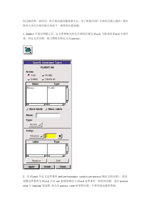
经过痛苦的一段经历,终于将局部问题真相大白,为了使保位同仁不再经过我之痛苦,现在将本人多孔介质经验公布如下,希望各位能加精:1。
Gambit中划分网格之后,定义需要做为多孔介质的区域为fluid,与缺省的fluid分别开来,再定义其名称,我习惯将名称定义为porous;2。
在fluent中定义边界条件define-boundary condition-porous(刚定义的名称),将其设置边界条件为fluid,点击set按钮即弹出与fluid边界条件一样的对话框,选中porous zone与laminar复选框,再点击porous zone标签即出现一个带有滚动条的界面;3。
porous zone设置方法:1)定义矢量:二维定义一个矢量,第二个矢量方向不用定义,是与第一个矢量方向正交的;三维定义二个矢量,第三个矢量方向不用定义,是与第一、二个矢量方向正交的;(如何知道矢量的方向:打开grid图,看看X,Y,Z的方向,如果是X向,矢量为1,0,0,同理Y向为0,1,0,Z向为0,0,1,如果所需要的方向与坐标轴正向相反,则定义矢量为负)圆锥坐标与球坐标请参考fluent帮助。
2)定义粘性阻力1/a与内部阻力C2:请参看本人上一篇博文“终于搞清fluent中多孔粘性阻力与内部阻力的计算方法”,此处不赘述;3)如果了定义粘性阻力1/a与内部阻力C2,就不用定义C1与C0,因为这是两种不同的定义方法,C1与C0只在幂率模型中出现,该处保持默认就行了;4)定义孔隙率porousity,默认值1表示全开放,此值按实验测值填写即可。
完了,其他设置与普通k-e或RSM相同。
总结一下,与君共享!Tutorial 7. Modeling Flow Through Porous MediaIntroductionMany industrial applications involve the modeling of flow through porous media, such as filters, catalyst beds, and packing. This tutorial illustrates how to set up and solve a problem involving gas flow through porous media.The industrial problem solved here involves gas flow through a catalytic converter. Catalytic converters are commonly used to purify emissions from gasoline and diesel engines by converting environmentally hazardous exhaust emissions to acceptable substances.Examples of such emissions include carbon monoxide (CO), nitrogen oxides (NOx), and unburned hydrocarbon fuels. These exhaust gas emissions are forced through a substrate, which is a ceramic structure coated with a metal catalyst such as platinum or palladium.The nature of the exhaust gas flow is a very important factor in determining the performance of the catalytic converter. Of particular importance is the pressure gradient and velocity distribution through the substrate. Hence CFD analysis is used to design efficient catalytic converters: by modeling the exhaust gas flow, the pressure drop and the uniformity of flow through the substrate can be determined. In this tutorial, FLUENT is used to model the flow of nitrogen gas through a catalytic converter geometry, so that the flow field structure may be analyzed.This tutorial demonstrates how to do the following:_ Set up a porous zone for the substrate with appropriate resistances._ Calculate a solution for gas flow through the catalytic converter using the pressure based solver. _ Plot pressure and velocity distribution on specified planes of the geometry._ Determine the pressure drop through the substrate and the degree of non-uniformity of flow through cross sections of the geometry using X-Y plots and numerical reports.Problem DescriptionThe catalytic converter modeled here is shown in Figure 7.1. The nitrogen flows in through the inlet with a uniform velocity of 22.6 m/s, passes through a ceramic monolith substrate with square shaped channels, and then exits through the outlet.While the flow in the inlet and outlet sections is turbulent, the flow through the substrate is laminar and is characterized by inertial and viscous loss coefficients in the flow (X) direction. The substrate is impermeable in other directions, which is modeled using loss coefficients whose values are three orders of magnitude higher than in the X direction.Setup and SolutionStep 1: Grid1. Read the mesh file (catalytic converter.msh).File /Read /Case...2. Check the grid. Grid /CheckFLUENT will perform various checks on the mesh and report the progress in the console. Make sure that the minimum volume reported is a positive number.3. Scale the grid.Grid! Scale...(a) Select mm from the Grid Was Created In drop-down list.(b) Click the Change Length Units button. All dimensions will now be shown in millimeters.(c) Click Scale and close the Scale Grid panel.4. Display the mesh. Display /Grid...(a) Make sure that inlet, outlet, substrate-wall, and wall are selected in the Surfaces selection list.(b) Click Display.(c) Rotate the view and zoom in to get the display shown in Figure 7.2.(d) Close the Grid Display panel.The hex mesh on the geometry contains a total of 34,580 cells.Step 2: Models1. Retain the default solver settings. Define /Models /Solver...2. Select the standard k-ε turbulence model. Define/ Models /Viscous...Step 3: Materials1. Add nitrogen to the list of fluid materials by copying it from the Fluent Database for materials.Define /Materials...(a) Click the Fluent Database... button to open the Fluent Database Materials panel.i. Select nitrogen (n2) from the list of Fluent Fluid Materials.ii. Click Copy to copy the information for nitrogen to your list of fluid materials. iii. Close the Fluent Database Materials panel.(b) Close the Materials panel.Step 4: Boundary Conditions. Define /Boundary Conditions...1. Set the boundary conditions for the fluid (fluid).(a) Select nitrogen from the Material Name drop-down list.(b) Click OK to close the Fluid panel.2. Set the boundary conditions for the substrate (substrate).(a) Select nitrogen from the Material Name drop-down list.(b) Enable the Porous Zone option to activate the porous zone model.(c) Enable the Laminar Zone option to solve the flow in the porous zone without turbulence.(d) Click the Porous Zone tab.i. Make sure that the principal direction vectors are set as shown in Table7.1. Use the scroll bar to access the fields that are not initially visible in the panel.ii. Enter the values in Table 7.2 for the Viscous Resistance and Inertial Resistance. Scroll down to access the fields that are not initially visible in the panel.(e) Click OK to close the Fluid panel.3. Set the velocity and turbulence boundary conditions at the inlet (inlet).(a) Enter 22.6 m/s for the Velocity Magnitude.(b) Select Intensity and Hydraulic Diameter from the Specification Method dropdown list in the Turbulence group box.(c) Retain the default value of 10% for the Turbulent Intensity.(d) Enter 42 mm for the Hydraulic Diameter.(e) Click OK to close the Velocity Inlet panel.4. Set the boundary conditions at the outlet (outlet).(a) Retain the default setting of 0 for Gauge Pressure.(b) Select Intensity and Hydraulic Diameter from the Specification Method dropdown list in the Turbulence group box.(c) Enter 5% for the Backflow Turbulent Intensity.(d) Enter 42 mm for the Backflow Hydraulic Diameter.(e) Click OK to close the Pressure Outlet panel.5. Retain the default boundary conditions for the walls (substrate-wall and wall) and close the Boundary Conditions panel.Step 5: Solution1. Set the solution parameters. Solve /Controls /Solution...(a) Retain the default settings for Under-Relaxation Factors.(b) Select Second Order Upwind from the Momentum drop-down list in the Discretization group box.(c) Click OK to close the Solution Controls panel.2. Enable the plotting of residuals during the calculation. Solve/Monitors /Residual...(a) Enable Plot in the Options group box.(b) Click OK to close the Residual Monitors panel.3. Enable the plotting of the mass flow rate at the outlet.Solve / Monitors /Surface...(a) Set the Surface Monitors to 1.(b) Enable the Plot and Write options for monitor-1, and click the Define... button to open the Define Surface Monitor panel.i. Select Mass Flow Rate from the Report Type drop-down list.ii. Select outlet from the Surfaces selection list.iii. Click OK to close the Define Surface Monitors panel.(c) Click OK to close the Surface Monitors panel.4. Initialize the solution from the inlet. Solve /Initialize /Initialize...(a) Select inlet from the Compute From drop-down list.(b) Click Init and close the Solution Initialization panel.5. Save the case file (catalytic converter.cas). File /Write /Case...6. Run the calculation by requesting 100 iterations. Solve /Iterate...(a) Enter 100 for the Number of Iterations.(b) Click Iterate.The FLUENT calculation will converge in approximately 70 iterations. By this point the mass flow rate monitor has attended out, as seen in Figure 7.3.(c) Close the Iterate panel.7. Save the case and data files (catalytic converter.cas and catalytic converter.dat).File /Write /Case & Data...Note: If you choose a file name that already exists in the current folder, FLUENTwill prompt you for confirmation to overwrite the file.Step 6: Post-processing1. Create a surface passing through the centerline for post-processing purposes.Surface/Iso-Surface...(a) Select Grid... and Y-Coordinate from the Surface of Constant drop-down lists.(b) Click Compute to calculate the Min and Max values.(c) Retain the default value of 0 for the Iso-Values.(d) Enter y=0 for the New Surface Name.(e) Click Create.2. Create cross-sectional surfaces at locations on either side of the substrate, as well as at its center.Surface /Iso-Surface...(a) Select Grid... and X-Coordinate from the Surface of Constant drop-down lists.(b) Click Compute to calculate the Min and Max values.(c) Enter 95 for Iso-Values.(d) Enter x=95 for the New Surface Name.(e) Click Create.(f) In a similar manner, create surfaces named x=130 and x=165 with Iso-Values of 130 and 165, respectively. Close the Iso-Surface panel after all the surfaces have been created.3. Create a line surface for the centerline of the porous media.Surface /Line/Rake...(a) Enter the coordinates of the line under End Points, using the starting coordinate of (95, 0, 0) and an ending coordinate of (165, 0, 0), as shown.(b) Enter porous-cl for the New Surface Name.(c) Click Create to create the surface.(d) Close the Line/Rake Surface panel.4. Display the two wall zones (substrate-wall and wall). Display /Grid...(a) Disable the Edges option.(b) Enable the Faces option.(c) Deselect inlet and outlet in the list under Surfaces, and make sure that only substrate-wall and wall are selected.(d) Click Display and close the Grid Display panel.(e) Rotate the view and zoom so that the display is similar to Figure 7.2.5. Set the lighting for the display. Display /Options...(a) Enable the Lights On option in the Lighting Attributes group box.(b) Retain the default selection of Gourand in the Lighting drop-down list.(c) Click Apply and close the Display Options panel.6. Set the transparency parameter for the wall zones (substrate-wall and wall).Display/Scene...(a) Select substrate-wall and wall in the Names selection list.(b) Click the Display... button under Geometry Attributes to open the Display Properties panel.i. Set the Transparency slider to 70.ii. Click Apply and close the Display Properties panel.(c) Click Apply and then close the Scene Description panel.7. Display velocity vectors on the y=0 surface.Display /Vectors...(a) Enable the Draw Grid option. The Grid Display panel will open.i. Make sure that substrate-wall and wall are selected in the list under Surfaces.ii. Click Display and close the Display Grid panel.(b) Enter 5 for the Scale.(c) Set Skip to 1.(d) Select y=0 from the Surfaces selection list.(e) Click Display and close the Vectors panel.The flow pattern shows that the flow enters the catalytic converter as a jet, with recirculation on either side of the jet. As it passes through the porous substrate, it decelerates and straightens out, and exhibits a more uniform velocity distribution.This allows the metal catalyst present in the substrate to be more effective.Figure 7.4: Velocity Vectors on the y=0 Plane8. Display filled contours of static pressure on the y=0 plane.Display /Contours...(a) Enable the Filled option.(b) Enable the Draw Grid option to open the Display Grid panel.i. Make sure that substrate-wall and wall are selected in the list under Surfaces.ii. Click Display and close the Display Grid panel.(c) Make sure that Pressure... and Static Pressure are selected from the Contours of drop-down lists.(d) Select y=0 from the Surfaces selection list.(e) Click Display and close the Contours panel.Figure 7.5: Contours of the Static Pressure on the y=0 planeThe pressure changes rapidly in the middle section, where the fluid velocity changes as it passes through the porous substrate. The pressure drop can be high, due to the inertial and viscous resistance of the porous media. Determining this pressure drop is a goal of CFD analysis. In the next step, you will learn how to plot the pressure drop along the centerline of the substrate.9. Plot the static pressure across the line surface porous-cl.Plot /XY Plot...(a) Make sure that the Pressure... and Static Pressure are selected from the Y Axis Function drop-down lists.(b) Select porous-cl from the Surfaces selection list.(c) Click Plot and close the Solution XY Plot panel.Figure 7.6: Plot of the Static Pressure on the porous-cl Line SurfaceIn Figure 7.6, the pressure drop across the porous substrate can be seen to be roughly 300 Pa.10. Display filled contours of the velocity in the X direction on the x=95, x=130 and x=165 surfaces.Display /Contours...(a) Disable the Global Range option.(b) Select Velocity... and X Velocity from the Contours of drop-down lists.(c) Select x=130, x=165, and x=95 from the Surfaces selection list, and deselect y=0.(d) Click Display and close the Contours panel.The velocity profile becomes more uniform as the fluid passes through the porous media. The velocity is very high at the center (the area in red) just before the nitrogen enters the substrate and then decreases as it passes through and exits the substrate. The area in green, which corresponds to a moderate velocity, increases in extent.Figure 7.7: Contours of the X Velocity on the x=95, x=130, and x=165 Surfaces11. Use numerical reports to determine the average, minimum, and maximum of the velocity distribution before and after the porous substrate.Report /Surface Integrals...(a) Select Mass-Weighted Average from the Report Type drop-down list.(b) Select Velocity and X Velocity from the Field Variable drop-down lists.(c) Select x=165 and x=95 from the Surfaces selection list.(d) Click Compute.(e) Select Facet Minimum from the Report Type drop-down list and click Compute again.(f) Select Facet Maximum from the Report Type drop-down list and click Compute again.(g) Close the Surface Integrals panel.The numerical report of average, maximum and minimum velocity can be seen in the main FLUENT console, as shown in the following example:The spread between the average, maximum, and minimum values for X velocity gives the degree to which the velocity distribution is non-uniform. You can also use these numbers to calculate the velocity ratio (i.e., the maximum velocity divided by the mean velocity) and the space velocity (i.e., the product of the mean velocity and the substrate length).Custom field functions and UDFs can be also used to calculate more complex measures ofnon-uniformity, such as the standard deviation and the gamma uniformity index.SummaryIn this tutorial, you learned how to set up and solve a problem involving gas flow through porous media in FLUENT. You also learned how to perform appropriate post-processing to investigate the flow field, determine the pressure drop across the porous media and non-uniformity of the velocity distribution as the fluid goes through the porous media.Further ImprovementsThis tutorial guides you through the steps to reach an initial solution. You may be able to obtain a more accurate solution by using an appropriate higher-order discretization scheme and by adapting the grid. Grid adaption can also ensure that the solution is independent of the grid. These steps aredemonstrated in Tutorial 1.。
Fluent经典教材.5.turbulence
ρU i
Convection
Generation
Diffusion
Dissipation Rate
ε2 ε ε ε U j U i U j ρU i + + = C1ε t C 2ε ρ ( t σ ε ) k x x xi x j i xi xi k i
D5
Fluent Inc. 6/18/2010
Fluent Software Training TRN-98-006
Choices to be Made
Flow Physics Computational Resources
Turbulence Model & Near-Wall Treatment
D9 Fluent Inc. 6/18/2010
Fluent Software Training TRN-98-006
One-Equation Model: Spalart-Allmaras
Designed specifically for aerospace applications involving wallbounded flows.
One Equation Model: Spalart-Allmaras
Turbulent viscosity is determined from:
~ (ν /ν )3 ~ t = ρν ~ 3 (ν /ν ) + cν 13
~ ν is determined from the modified viscosity transport equation:
- 1、下载文档前请自行甄别文档内容的完整性,平台不提供额外的编辑、内容补充、找答案等附加服务。
- 2、"仅部分预览"的文档,不可在线预览部分如存在完整性等问题,可反馈申请退款(可完整预览的文档不适用该条件!)。
- 3、如文档侵犯您的权益,请联系客服反馈,我们会尽快为您处理(人工客服工作时间:9:00-18:30)。
2 / 53
Fluent Inc. 6/7/2005
Fluent User Services Center
Advanced Fluent Training Turbulence Apr 2005
Importance of Near-Wall Turbulence
Viscous sublayer
dimensional analysis U = f(ρ, τ, , y) U = uτf(y+)
– uτ = (τw/ρ)1/2
– y+ = yuτ/ν Clauser defect layer
U = Ue - uτg(η) – η = y/
Local turbulent equilibrium k = uτ2/C1/2 ε = uτ3/κy Precludes transport of turbulence in log layer
3 / 53
Fluent Inc. 6/7/2005
Fluent User SeTraining Turbulence Apr 2005
Near-Wall Modeling Issues
k-ε and RSM models are valid in the turbulent core region and through the log layer
ρ C 1/ 4k 1/ 2 yP P y ≡
Similar ‘wall laws’ apply for energy and species. Cell center is immersed in log layer Local equilibrium (production = dissipation) prevails kn = 0 at surface
k and ε functions of uτ only
Overlap layer
large scale variance (ν /uτ<< ) uτf(y+) = Ue - uτg(η) uτ2f′(y+)/ν = -uτg′(η)/ or ( x y/uτ ) y+f′(y+) = -ηg′(η) U 1 u + = ln( y + ) + C ; u + = κ uτ
Fluent User Services Center
Advanced Fluent Training Turbulence Apr 2005
Topics to be discussed
Near wall modeling options Low Reynolds number turbulence models Large Eddy Simulation (LES) and Detached Eddy Simulation (DES)
Severe p Transpiration through wall strong body forces highly 3D flow rapidly changing fluid properties near wall
Low-Re flows are pervasive throughout model Small gaps are present
k production and dissipation are nearly equal in overlap layer
‘turbulent equilibrium’
dissipation >> production in sublayer region
Fluent Inc. 6/7/2005
Forcing (Production = Dissipation) over (Production << Dissipation)
8 / 53
Fluent Inc. 6/7/2005
Fluent User Services Center
Advanced Fluent Training Turbulence Apr 2005
Fluent User Services Center
Advanced Fluent Training Turbulence Apr 2005
Near-Wall Modeling Options
In general, ‘wall functions’ are a collection or set of laws that serve as boundary conditions for momentum, energy, and species as well as for turbulence quantities Wall Function Options
U = U(ρ, τ, , y, k )
Introduces additional velocity scale for ‘general’ application
U = y for U = 1 ln Ey κ
* y* < yv UP C 1/ 4k 1/ 2 P * * where U ≡ y > yv τw / ρ
Enhanced Wall Treatment or Low-Re Option
This near-wall model combines the use of enhanced wall functions and a two-layer model
Used for low-Re flows or flows with complex near-wall phenomena Generally requires a very fine near-wall mesh capable of resolving the near-wall region Turbulence models are modified for ‘inner’ layer
Velocity profile exhibits layer structure identified from dimensional analysis
Inner layer viscous forces rule, U = f(ρ, τw, , y) Outer layer dependent upon mean flow Overlap layer log-law applies 5 / 53
Fluent Inc. 6/7/2005
Fluent User Services Center
Advanced Fluent Training Turbulence Apr 2005
Flow Behavior in Near-Wall Region
U/uτ k
Near-wall flows are anisotropic due to presence of walls
Special near-wall treatments are necessary since equations cannot be integrated down to wall
4 / 53
Generally, k is obtained from solution of k transport equation
ε calculated at wall-adjacent cells using local equilibrium assumption
ε = C3/4k3/2/κy
Wall functions less reliable when cell intrudes viscous sublayer
Fluent User Services Center
Advanced Fluent Training Turbulence Apr 2005
Turbulence Modeling Options in FLUENT
1 / 53
Fluent Inc. 6/7/2005
Walls are main source of vorticity and turbulence Accurate near-wall modeling is important for most engineering applications
Successful prediction of frictional drag for external flows, or pressure drop for internal flows, depends on fidelity of local wall shear predictions Pressure drag for bluff bodies is dependent upon extent of separation Thermal performance of heat exchangers, etc., is determined by wall heat transfer whose prediction depends upon near-wall effects
6 / 53
outer layer inner layer
Fluent Inc. 6/7/2005
Fluent User Services Center
Advanced Fluent Training Turbulence Apr 2005
Wall Functions
Limitations of Standard Wall Functions
Wall functions become less reliable when flow departs from the conditions assumed in their derivation:
Local equilibrium assumption fails