On the maximum of r-Stirling numbers
浅谈Stirling数极其简单应用

摘要组合数学中的许多问题是数学中的精华,组合数学的应用也涉及到自然科学的许多领域。
本文对Stirling数进行了研究。
本文的工作分为三部分:第一部分,介绍了Stirling数的概念和性质;第二部分列举了关于两类Stirling数之间的几个关系式。
重点介绍了两类Stirling阵之间的关系,并分别用Stirling阵和Stirling展开式证明了两类Stirling数的反演和互逆关系;第三部分则简单介绍了两类Stirling数的简单应用。
关键词:Stirling数;基本性质;关系;简单应用AbstractThe problems in combination of mathematics is the essence of mathematics.the application of combination of mathematics relates to many fields of natural science.This paper is divided into three parts: the first part,introduces the concept and the characteristics of Stirling number ; the second part lists several relations which is about two Stirling number . It focuses on the relations between the two types of Stirling array, using the Stirling matrix and Stirling expansion to proved the inversion and reciprocal relationship of the two kinds of Stirling numbers; the third part introduces the simple application of the two kinds of the Stirling numbers.Keywords Stirling number; basic characteristics; relations; simple application目录引言 (4)第一章 Stirling数的概念及其性质 (2)1.1 第一类、第二类Stirling函数的概念 (2)1.2 两类Stirling函数的性质 (3)1.3 两类Stirling数的解析表达式 (5)第二章两类Stirling数之间的关系式 (7)2.1 两类Stirling数之间的反演关系 (7)2.2 两类Stirling阵之间的关系 (8)第三章 Stirling数的推广和简单应用 (11)3.1 第一类Stirling数简单应用 (11)3.2 利用第二类Stirling数分配计数 (11)总结 (13)参考文献 (14)谢辞 (15)引言组合数学是既古老又年轻的数学分支,她的渊源可以追溯到公元前2200年中国的大禹治水时代,中外历史上许多著名的数学游戏是她古典部分的主要内容。
ASTM D 790-2007(弯曲)
Designation:D790–07Standard Test Methods forFlexural Properties of Unreinforced and Reinforced Plastics and Electrical Insulating Materials1This standard is issued under thefixed designation D790;the number immediately following the designation indicates the year of original adoption or,in the case of revision,the year of last revision.A number in parentheses indicates the year of last reapproval.A superscript epsilon(e)indicates an editorial change since the last revision or reapproval.This standard has been approved for use by agencies of the Department of Defense.1.Scope*1.1These test methods cover the determination offlexural properties of unreinforced and reinforced plastics,including high-modulus composites and electrical insulating materials in the form of rectangular bars molded directly or cut from sheets, plates,or molded shapes.These test methods are generally applicable to both rigid and semirigid materials.However,flexural strength cannot be determined for those materials that do not break or that do not fail in the outer surface of the test specimen within the5.0%strain limit of these test methods. These test methods utilize a three-point loading system applied to a simply supported beam.A four-point loading system method can be found in Test Method D6272.1.1.1Procedure A,designed principally for materials that break at comparatively small deflections.1.1.2Procedure B,designed particularly for those materials that undergo large deflections during testing.1.1.3Procedure A shall be used for measurement offlexural properties,particularlyflexural modulus,unless the material specification states otherwise.Procedure B may be used for measurement offlexural strength only.Tangent modulus data obtained by Procedure A tends to exhibit lower standard deviations than comparable data obtained by means of Proce-dure B.1.2Comparative tests may be run in accordance with either procedure,provided that the procedure is found satisfactory for the material being tested.1.3The values stated in SI units are to be regarded as the standard.The values provided in brackets are for information only.1.4This standard does not purport to address all of the safety concerns,if any,associated with its use.It is the responsibility of the user of this standard to establish appro-priate safety and health practices and determine the applica-bility of regulatory limitations prior to use.N OTE1—These test methods are not technically equivalent to ISO178.2.Referenced Documents2.1ASTM Standards:2D618Practice for Conditioning Plastics for TestingD638Test Method for Tensile Properties of PlasticsD883Terminology Relating to PlasticsD4000Classification System for Specifying Plastic Mate-rialsD4101Specification for Polypropylene Injection and Ex-trusion MaterialsD5947Test Methods for Physical Dimensions of Solid Plastics SpecimensD6272Test Method for Flexural Properties of Unrein-forced and Reinforced Plastics and Electrical Insulating Materials by Four-Point BendingE4Practices for Force Verification of Testing Machines E691Practice for Conducting an Interlaboratory Study to Determine the Precision of a Test Method2.2ISO Standard:3ISO178Plastics—Determination of Flexural Properties of Rigid Plastics3.Terminology3.1Definitions—Definitions of terms applying to these test methods appear in Terminology D883and Annex A1of Test Method D638.4.Summary of Test Method4.1A bar of rectangular cross section rests on two supports and is loaded by means of a loading nose midway between the supports.A support span-to-depth ratio of16:1shall be used unless there is reason to suspect that a larger span-to-depth ratio may be required,as may be the case for certain laminated materials(see Section7and Note7for guidance).1These test methods are under the jurisdiction of ASTM Committee D20on Plastics and are the direct responsibility of Subcommittee D20.10on Mechanical Properties.Current edition approved Sept.1,2007.Published October2007.Originally approved st previous edition approved in2003as D790–03.2For referenced ASTM standards,visit the ASTM website,,or contact ASTM Customer Service at service@.For Annual Book of ASTM Standards volume information,refer to the standard’s Document Summary page on the ASTM website.3Available from American National Standards Institute(ANSI),25W.43rd St., 4th Floor,New York,NY10036,.*A Summary of Changes section appears at the end of this standard. Copyright©ASTM International,100Barr Harbor Drive,PO Box C700,West Conshohocken,PA19428-2959,United States.4.2The specimen is deflected until rupture occurs in the outer surface of the test specimen or until a maximum strain (see 12.7)of5.0%is reached,whichever occurs first.4.3Procedure A employs a strain rate of 0.01mm/mm/min [0.01in./in./min]and is the preferred procedure for this test method,while Procedure B employs a strain rate of 0.10mm/mm/min [0.10in./in./min].5.Significance and Use5.1Flexural properties as determined by these test methods are especially useful for quality control and specification purposes.5.2Materials that do not fail by the maximum strain allowed under these test methods (3-point bend)may be more suited to a 4-point bend test.The basic difference between the two test methods is in the location of the maximum bending moment and maximum axial fiber stresses.The maximum axial fiber stresses occur on a line under the loading nose in 3-point bending and over the area between the loading noses in 4-point bending.5.3Flexural properties may vary with specimen depth,temperature,atmospheric conditions,and the difference in rate of straining as specified in Procedures A and B (see also Note 7).5.4Before proceeding with these test methods,reference should be made to the ASTM specification of the material being tested.Any test specimen preparation,conditioning,dimensions,or testing parameters,or combination thereof,covered in the ASTM material specification shall take prece-dence over those mentioned in these test methods.Table 1in Classification System D 4000lists the ASTM material speci-fications that currently exist for plastics.6.Apparatus6.1Testing Machine —A properly calibrated testing ma-chine that can be operated at constant rates of crosshead motion over the range indicated,and in which the error in the load measuring system shall not exceed 61%of the maximum load expected to be measured.It shall be equipped with a deflection measuring device.The stiffness of the testing machine shall be such that the total elastic deformation of the system does not exceed 1%of the total deflection of the test specimen duringtesting,or appropriate corrections shall be made.The load indicating mechanism shall be essentially free from inertial lag at the crosshead rate used.The accuracy of the testing machine shall be verified in accordance with Practices E 4.6.2Loading Noses and Supports —The loading nose and supports shall have cylindrical surfaces.The default radii of the loading nose and supports shall be 5.060.1mm [0.19760.004in.]unless otherwise specified in an ASTM material specification or as agreed upon between the interested parties.When the use of an ASTM material specification,or an agreed upon modification,results in a change to the radii of the loading nose and supports,the results shall be clearly identified as being obtained from a modified version of this test method and shall include the specification (when available)from which the modification was specified,for example,Test Method D 790in accordance with Specification D 4101.6.2.1Other Radii for Loading Noses and Supports —When other than default loading noses and supports are used,in order to avoid excessive indentation,or failure due to stress concen-tration directly under the loading nose,they must comply with the following requirements:they shall have a minimum radius of 3.2mm [1⁄8in.]for all specimens.For specimens 3.2mm or greater in depth,the radius of the supports may be up to 1.6times the specimen depth.They shall be this large if significant indentation or compressive failure occurs.The arc of the loading nose in contact with the specimen shall be sufficiently large to prevent contact of the specimen with the sides of the nose.The maximum radius of the loading nose shall be no more than four times the specimen depth.6.3Micrometers —Suitable micrometers for measuring the width and thickness of the test specimen to an incremental discrimination of at least 0.025mm [0.001in.]should be used.All width and thickness measurements of rigid and semirigid plastics may be measured with a hand micrometer with ratchet.A suitable instrument for measuring the thickness of nonrigid test specimens shall have:a contact measuring pressure of 2562.5kPa [3.660.36psi],a movable circular contact foot 6.3560.025mm [0.25060.001in.]in diameter and a lower fixed anvil large enough to extend beyond the contact foot in all directions and being parallel to the contact foot within 0.005mm [0.002in.]over the entire foot area.Flatness of foot and anvil shall conform to the portion of the Calibration section of Test Methods D 5947.7.Test Specimens7.1The specimens may be cut from sheets,plates,or molded shapes,or may be molded to the desired finished dimensions.The actual dimensions used in Section 4.2,Cal-culation,shall be measured in accordance with Test Methods D 5947.N OTE 2—Any necessary polishing of specimens shall be done only in the lengthwise direction of the specimen.7.2Sheet Materials (Except Laminated Thermosetting Ma-terials and Certain Materials Used for Electrical Insulation,Including Vulcanized Fiber and Glass Bonded Mica):7.2.1Materials 1.6mm [1⁄16in.]or Greater in Thickness —For flatwise tests,the depth of the specimen shall be the thickness of the material.For edgewise tests,the width of theTABLE 1Flexural StrengthMaterial Mean,103psiValues Expressed in Units of %of 103psi V r A V R B r C R D ABS9.99 1.59 6.05 4.4417.2DAP thermoset 14.3 6.58 6.5818.618.6Cast acrylic 16.3 1.6711.3 4.7332.0GR polyester19.5 1.43 2.14 4.05 6.08GR polycarbonate 21.0 5.16 6.0514.617.1SMC26.04.767.1913.520.4AV r =within-laboratory coefficient of variation for the indicated material.It is obtained by first pooling the within-laboratory standard deviations of the test results from all of the participating laboratories:Sr =[[(s 1)2+(s 2)2...+(s n )2]/n]1/2then V r =(S r divided by the overall average for the material)3100.BV r =between-laboratory reproducibility,expressed as the coefficient of varia-tion:S R ={S r 2+S L 2}1/2where S L is the standard deviation of laboratory means.Then:V R =(S R divided by the overall average for the material)3100.Cr =within-laboratory critical interval between two test results =2.83V r .DR =between-laboratory critical interval between two test results =2.83V R.specimen shall be the thickness of the sheet,and the depth shall not exceed the width(see Notes3and4).For all tests,the support span shall be16(tolerance61)times the depth of the beam.Specimen width shall not exceed one fourth of the support span for specimens greater than3.2mm[1⁄8in.]in depth.Specimens3.2mm or less in depth shall be12.7mm[1⁄2 in.]in width.The specimen shall be long enough to allow for overhanging on each end of at least10%of the support span, but in no case less than6.4mm[1⁄4in.]on each end.Overhang shall be sufficient to prevent the specimen from slipping through the supports.N OTE3—Whenever possible,the original surface of the sheet shall be unaltered.However,where testing machine limitations make it impossible to follow the above criterion on the unaltered sheet,one or both surfaces shall be machined to provide the desired dimensions,and the location of the specimens with reference to the total depth shall be noted.The value obtained on specimens with machined surfaces may differ from those obtained on specimens with original surfaces.Consequently,any specifi-cations forflexural properties on thicker sheets must state whether the original surfaces are to be retained or not.When only one surface was machined,it must be stated whether the machined surface was on the tension or compression side of the beam.N OTE4—Edgewise tests are not applicable for sheets that are so thin that specimens meeting these requirements cannot be cut.If specimen depth exceeds the width,buckling may occur.7.2.2Materials Less than1.6mm[1⁄16in.]in Thickness—The specimen shall be50.8mm[2in.]long by12.7mm[1⁄2in.] wide,testedflatwise on a25.4-mm[1-in.]support span.N OTE5—Use of the formulas for simple beams cited in these test methods for calculating results presumes that beam width is small in comparison with the support span.Therefore,the formulas do not apply rigorously to these dimensions.N OTE6—Where machine sensitivity is such that specimens of these dimensions cannot be measured,wider specimens or shorter support spans,or both,may be used,provided the support span-to-depth ratio is at least14to1.All dimensions must be stated in the report(see also Note5).7.3Laminated Thermosetting Materials and Sheet and Plate Materials Used for Electrical Insulation,Including Vulcanized Fiber and Glass-Bonded Mica—For paper-base and fabric-base grades over25.4mm[1in.]in nominal thickness,the specimens shall be machined on both surfaces to a depth of25.4mm.For glass-base and nylon-base grades, specimens over12.7mm[1⁄2in.]in nominal depth shall be machined on both surfaces to a depth of12.7mm.The support span-to-depth ratio shall be chosen such that failures occur in the outerfibers of the specimens,due only to the bending moment(see Note7).Therefore,a ratio larger than16:1may be necessary(32:1or40:1are recommended).When laminated materials exhibit low compressive strength perpendicular to the laminations,they shall be loaded with a large radius loading nose(up to four times the specimen depth to prevent premature damage to the outerfibers.7.4Molding Materials(Thermoplastics and Thermosets)—The recommended specimen for molding materials is127by 12.7by3.2mm[5by1⁄2by1⁄8in.]testedflatwise on a support span,resulting in a support span-to-depth ratio of16(tolerance 61).Thicker specimens should be avoided if they exhibit significant shrink marks or bubbles when molded.7.5High-Strength Reinforced Composites,Including Highly Orthotropic Laminates—The span-to-depth ratio shall be cho-sen such that failure occurs in the outerfibers of the specimens and is due only to the bending moment(see Note7).A span-to-depth ratio larger than16:1may be necessary(32:1or 40:1are recommended).For some highly anisotropic compos-ites,shear deformation can significantly influence modulus measurements,even at span-to-depth ratios as high as40:1. Hence,for these materials,an increase in the span-to-depth ratio to60:1is recommended to eliminate shear effects when modulus data are required,it should also be noted that the flexural modulus of highly anisotropic laminates is a strong function of ply-stacking sequence and will not necessarily correlate with tensile modulus,which is not stacking-sequence dependent.N OTE7—As a general rule,support span-to-depth ratios of16:1are satisfactory when the ratio of the tensile strength to shear strength is less than8to1,but the support span-to-depth ratio must be increased for composite laminates having relatively low shear strength in the plane of the laminate and relatively high tensile strength parallel to the support span.8.Number of Test Specimens8.1Test at leastfive specimens for each sample in the case of isotropic materials or molded specimens.8.2For each sample of anisotropic material in sheet form, test at leastfive specimens for each of the following conditions. Recommended conditions areflatwise and edgewise tests on specimens cut in lengthwise and crosswise directions of the sheet.For the purposes of this test,“lengthwise”designates the principal axis of anisotropy and shall be interpreted to mean the direction of the sheet known to be stronger inflexure.“Cross-wise”indicates the sheet direction known to be the weaker in flexure and shall be at90°to the lengthwise direction.9.Conditioning9.1Conditioning—Condition the test specimens at236 2°C[73.463.6°F]and5065%relative humidity for not less than40h prior to test in accordance with Procedure A of Practice D618unless otherwise specified by contract or the relevant ASTM material specification.Reference pre-test con-ditioning,to settle disagreements,shall apply tolerances of 61°C[1.8°F]and62%relative humidity.9.2Test Conditions—Conduct the tests at2362°C[73.46 3.6°F]and5065%relative humidity unless otherwise specified by contract or the relevant ASTM material specifica-tion.Reference testing conditions,to settle disagreements, shall apply tolerances of61°C[1.8°F]and62%relative humidity.10.Procedure10.1Procedure A:10.1.1Use an untested specimen for each measurement. Measure the width and depth of the specimen to the nearest 0.03mm[0.001in.]at the center of the support span.For specimens less than2.54mm[0.100in.]in depth,measure the depth to the nearest0.003mm[0.0005in.].These measure-ments shall be made in accordance with Test Methods D5947.10.1.2Determine the support span to be used as described in Section7and set the support span to within1%of the determinedvalue.10.1.3Forflexuralfixtures that have continuously adjust-able spans,measure the span accurately to the nearest0.1mm [0.004in.]for spans less than63mm[2.5in.]and to the nearest 0.3mm[0.012in.]for spans greater than or equal to63mm [2.5in.].Use the actual measured span for all calculations.For flexuralfixtures that havefixed machined span positions,verify the span distance the same as for adjustable spans at each machined position.This distance becomes the span for that position and is used for calculations applicable to all subse-quent tests conducted at that position.See Annex A2for information on the determination of and setting of the span.10.1.4Calculate the rate of crosshead motion as follows and set the machine for the rate of crosshead motion as calculated by Eq1:R5ZL2/6d(1) where:R=rate of crosshead motion,mm[in.]/min,L=support span,mm[in.],d=depth of beam,mm[in.],andZ=rate of straining of the outerfiber,mm/mm/min[in./ in./min].Z shall be equal to0.01.In no case shall the actual crosshead rate differ from that calculated using Eq1,by more than610%.10.1.5Align the loading nose and supports so that the axes of the cylindrical surfaces are parallel and the loading nose is midway between the supports.The parallelism of the apparatus may be checked by means of a plate with parallel grooves into which the loading nose and supports willfit when properly aligned(see A2.3).Center the specimen on the supports,with the long axis of the specimen perpendicular to the loading nose and supports.10.1.6Apply the load to the specimen at the specified crosshead rate,and take simultaneous load-deflection data. Measure deflection either by a gage under the specimen in contact with it at the center of the support span,the gage being mounted stationary relative to the specimen supports,or by measurement of the motion of the loading nose relative to the supports.Load-deflection curves may be plotted to determine theflexural strength,chord or secant modulus or the tangent modulus of elasticity,and the total work as measured by the area under the load-deflection curve.Perform the necessary toe compensation(see Annex A1)to correct for seating and indentation of the specimen and deflections in the machine.10.1.7Terminate the test when the maximum strain in the outer surface of the test specimen has reached0.05mm/mm [in./in.]or at break if break occurs prior to reaching the maximum strain(Notes8and9).The deflection at which this strain will occur may be calculated by letting r equal0.05 mm/mm[in./in.]in Eq2:D5rL2/6d(2) where:D=midspan deflection,mm[in.],r=strain,mm/mm[in./in.],L=support span,mm[in.],andd=depth of beam,mm[in.].N OTE8—For some materials that do not yield or break within the5% strain limit when tested by Procedure A,the increased strain rate allowed by Procedure B(see10.2)may induce the specimen to yield or break,or both,within the required5%strain limit.N OTE9—Beyond5%strain,this test method is not applicable.Some other mechanical property might be more relevant to characterize mate-rials that neither yield nor break by either Procedure A or Procedure B within the5%strain limit(for example,Test Method D638may be considered).10.2Procedure B:10.2.1Use an untested specimen for each measurement.10.2.2Test conditions shall be identical to those described in10.1,except that the rate of straining of the outer surface of the test specimen shall be0.10mm/mm[in./in.]/min.10.2.3If no break has occurred in the specimen by the time the maximum strain in the outer surface of the test specimen has reached0.05mm/mm[in./in.],discontinue the test(see Note9).11.Retests11.1Values for properties at rupture shall not be calculated for any specimen that breaks at some obvious,fortuitousflaw, unless suchflaws constitute a variable being studied.Retests shall be made for any specimen on which values are not calculated.12.Calculation12.1Toe compensation shall be made in accordance with Annex A1unless it can be shown that the toe region of the curve is not due to the take-up of slack,seating of the specimen,or other artifact,but rather is an authentic material response.12.2Flexural Stress(s f)—When a homogeneous elastic material is tested inflexure as a simple beam supported at two points and loaded at the midpoint,the maximum stress in the outer surface of the test specimen occurs at the midpoint.This stress may be calculated for any point on the load-deflection curve by means of the following equation(see Notes10-12):s f53PL/2bd2(3) where:s=stress in the outerfibers at midpoint,MPa[psi],P=load at a given point on the load-deflection curve,N [lbf],L=support span,mm[in.],b=width of beam tested,mm[in.],andd=depth of beam tested,mm[in.].N OTE10—Eq3applies strictly to materials for which stress is linearly proportional to strain up to the point of rupture and for which the strains are small.Since this is not always the case,a slight error will be introduced if Eq3is used to calculate stress for materials that are not true Hookean materials.The equation is valid for obtaining comparison data and for specification purposes,but only up to a maximumfiber strainof5%in the outer surface of the test specimen for specimens tested by the procedures described herein.N OTE11—When testing highly orthotropic laminates,the maximum stress may not always occur in the outer surface of the test specimen.4 Laminated beam theory must be applied to determine the maximum tensile stress at failure.If Eq3is used to calculate stress,it will yield an apparent strength based on homogeneous beam theory.This apparent strength is highly dependent on the ply-stacking sequence of highly orthotropic laminates.N OTE12—The preceding calculation is not valid if the specimen slips excessively between the supports.12.3Flexural Stress for Beams Tested at Large Support Spans(s f)—If support span-to-depth ratios greater than16to 1are used such that deflections in excess of10%of the support span occur,the stress in the outer surface of the specimen for a simple beam can be reasonably approximated with the following equation(see Note13):s f5~3PL/2bd2!@116~D/L!224~d/L!~D/L!#(4) where:s f,P,L,b,and d are the same as for Eq3,andD=deflection of the centerline of the specimen at the middle of the support span,mm[in.].N OTE13—When large support span-to-depth ratios are used,significant end forces are developed at the support noses which will affect the moment in a simple supported beam.Eq4includes additional terms that are an approximate correction factor for the influence of these end forces in large support span-to-depth ratio beams where relatively large deflec-tions exist.12.4Flexural Strength(s fM)—Maximumflexural stress sustained by the test specimen(see Note11)during a bendingtest.It is calculated according to Eq3or Eq4.Some materials that do not break at strains of up to5%may give a load deflection curve that shows a point at which the load does not increase with an increase in strain,that is,a yield point(Fig.1, Curve B),Y.Theflexural strength may be calculated for these materials by letting P(in Eq3or Eq4)equal this point,Y.12.5Flexural Offset Yield Strength—Offset yield strength is the stress at which the stress-strain curve deviates by a given strain(offset)from the tangent to the initial straight line portion of the stress-strain curve.The value of the offset must be given whenever this property is calculated.N OTE14—This value may differ fromflexural strength defined in12.4. Both methods of calculation are described in the annex to Test Method D638.12.6Flexural Stress at Break(s fB)—Flexural stress at break of the test specimen during a bending test.It is calculated according to Eq3or Eq4.Some materials may give a load deflection curve that shows a break point,B,without a yield point(Fig.1,Curve a)in which case s fB=s fM.Other materials may give a yield deflection curve with both a yield and a break point,B(Fig.1,Curve b).Theflexural stress at break may be calculated for these materials by letting P(in Eq 3or Eq4)equal this point,B.12.7Stress at a Given Strain—The stress in the outer surface of a test specimen at a given strain may be calculated in accordance with Eq3or Eq4by letting P equal the load read from the load-deflection curve at the deflection corresponding to the desired strain(for highly orthotropic laminates,see Note11).12.8Flexural Strain,e f—Nominal fractional change in the length of an element of the outer surface of the test specimen at midspan,where the maximum strain occurs.It may be calculated for any deflection using Eq5:e f56Dd/L2(5) where:e f=strain in the outer surface,mm/mm[in./in.],D=maximum deflection of the center of the beam,mm [in.],L=support span,mm[in.],andd=depth,mm[in.].12.9Modulus of Elasticity:12.9.1Tangent Modulus of Elasticity—The tangent modu-lus of elasticity,often called the“modulus of elasticity,”is the ratio,within the elastic limit,of stress to corresponding strain. It is calculated by drawing a tangent to the steepest initial straight-line portion of the load-deflection curve and using Eq 6(for highly anisotropic composites,see Note15).E B5L3m/4bd3(6)4For a discussion of these effects,see Zweben,C.,Smith,W.S.,and Wardle,M. W.,“Test Methods for Fiber Tensile Strength,Composite Flexural Modulus and Properties of Fabric-Reinforced Laminates,“Composite Materials:Testing and Design(Fifth Conference),ASTM STP674,1979,pp.228–262.N OTE—Curve a:Specimen that breaks before yielding.Curve b:Specimen that yields and then breaks before the5%strain limit.Curve c:Specimen that neither yields nor breaks before the5%strain limit.FIG.1Typical Curves of Flexural Stress(ßf)Versus FlexuralStrain(ef)where:E B =modulus of elasticity in bending,MPa [psi],L =support span,mm [in.],b =width of beam tested,mm [in.],d =depth of beam tested,mm [in.],andm =slope of the tangent to the initial straight-line portion of the load-deflection curve,N/mm [lbf/in.]of deflec-tion.N OTE 15—Shear deflections can seriously reduce the apparent modulusof highly anisotropic composites when they are tested at low span-to-depth ratios.4For this reason,a span-to-depth ratio of 60to 1is recommended for flexural modulus determinations on these composites.Flexural strength should be determined on a separate set of replicate specimens at a lower span-to-depth ratio that induces tensile failure in the outer fibers of the beam along its lower face.Since the flexural modulus of highly anisotropic laminates is a critical function of ply-stacking sequence,it will not necessarily correlate with tensile modulus,which is not stacking-sequence dependent.12.9.2Secant Modulus —The secant modulus is the ratio of stress to corresponding strain at any selected point on the stress-strain curve,that is,the slope of the straight line that joins the origin and a selected point on the actual stress-strain curve.It shall be expressed in megapascals [pounds per square inch].The selected point is chosen at a prespecified stress or strain in accordance with the appropriate material specification or by customer contract.It is calculated in accordance with Eq 6by letting m equal the slope of the secant to the load-deflection curve.The chosen stress or strain point used for the determination of the secant shall be reported.12.9.3Chord Modulus (E f )—The chord modulus may be calculated from two discrete points on the load deflection curve.The selected points are to be chosen at two prespecified stress or strain points in accordance with the appropriate material specification or by customer contract.The chosen stress or strain points used for the determination of the chord modulus shall be reported.Calculate the chord modulus,E f using the following equation:E f 5~s f 22s f 1!/~e f 22e f 1!(7)where:s f 2and s f 1are the flexural stresses,calculated from Eq 3or Eq 4and measured at the predefined points on the loaddeflection curve,and e f 2ande f 1are the flexural strain values,calculated from Eq 5and measured at the predetermined points on the load deflection curve.12.10Arithmetic Mean —For each series of tests,the arithmetic mean of all values obtained shall be calculated to three significant figures and reported as the “average value”for the particular property in question.12.11Standard Deviation —The standard deviation (esti-mated)shall be calculated as follows and be reported to two significant figures:s 5=~(X 22nX¯2!/~n 21!(8)where:s =estimated standard deviation,X =value of single observation,n =number of observations,andX ¯=arithmetic mean of the set of observations.13.Report13.1Report the following information:13.1.1Complete identification of the material tested,includ-ing type,source,manufacturer’s code number,form,principal dimensions,and previous history (for laminated materials,ply-stacking sequence shall be reported),13.1.2Direction of cutting and loading specimens,when appropriate,13.1.3Conditioning procedure,13.1.4Depth and width of specimen,13.1.5Procedure used (A or B),13.1.6Support span length,13.1.7Support span-to-depth ratio if different than 16:1,13.1.8Radius of supports and loading noses,if different than 5mm.When support and/or loading nose radii other than 5mm are used,the results shall be identified as being generated by a modified version of this test method and the referring specification referenced as to the geometry used.13.1.9Rate of crosshead motion,13.1.10Flexural strain at any given stress,average value and standard deviation,13.1.11If a specimen is rejected,reason(s)for rejection,13.1.12Tangent,secant,or chord modulus in bending,average value,standard deviation,and the strain level(s)used if secant or chord modulus,13.1.13Flexural strength (if desired),average value,and standard deviation,13.1.14Stress at any given strain up to and including 5%(if desired),with strain used,average value,and standard devia-tion,13.1.15Flexural stress at break (if desired),average value,and standard deviation,13.1.16Type of behavior,whether yielding or rupture,or both,or other observations,occurring within the 5%strain limit,and13.1.17Date of specific version of test used.TABLE 2Flexural ModulusMaterial Mean,103psiValues Expressed in units of %of 103psi V r A V R B r C R D ABS338 4.797.6913.621.8DAP thermoset 485 2.897.188.1520.4Cast acrylic 81013.716.138.845.4GR polyester816 3.49 4.209.9111.9GR polycarbonate 1790 5.52 5.5215.615.6SMC195010.913.830.839.1AV r =within-laboratory coefficient of variation for the indicated material.It is obtained by first pooling the within-laboratory standard deviations of the test results from all of the participating laboratories:Sr =[[(s 1)2+(s 2)2...+(s n )2]/n ]1/2then V r =(S r divided by the overall average for the material)3100.BV r =between-laboratory reproducibility,expressed as the coefficient of varia-tion:S R ={S r 2+S L 2}1/2where S L is the standard deviation of laboratory means.Then:V R =(S R divided by the overall average for the material)3100.Cr =within-laboratory critical interval between two test results =2.83V r .DR =between-laboratory critical interval between two test results =2.83V R.。
TPS61040中文资料

V O = 18 V200 µS/divFigure 12. Line Transient ResponseV O = 18 V200 µS/div Figure 13. Load Transient ResponseV O = 18 VFigure 14. Start-Up BehaviorIMPORTANT NOTICETexas Instruments Incorporated and its subsidiaries (TI) reserve the right to make corrections, modifications, enhancements, improvements, and other changes to its products and services at any time and to discontinue any product or service without notice. Customers should obtain the latest relevant information before placing orders and should verify that such information is current and complete. All products are sold subject to TI’s terms and conditions of sale supplied at the time of order acknowledgment.TI warrants performance of its hardware products to the specifications applicable at the time of sale in accordance with TI’s standard warranty. Testing and other quality control techniques are used to the extent TI deems necessary to support this warranty. Except where mandated by government requirements, testing of all parameters of each product is not necessarily performed.TI assumes no liability for applications assistance or customer product design. Customers are responsible for their products and applications using TI components. To minimize the risks associated with customer products and applications, customers should provide adequate design and operating safeguards.TI does not warrant or represent that any license, either express or implied, is granted under any TI patent right, copyright, mask work right, or other TI intellectual property right relating to any combination, machine, or process in which TI products or services are used. Information published by TI regarding third–party products or services does not constitute a license from TI to use such products or services or a warranty or endorsement thereof. Use of such information may require a license from a third party under the patents or other intellectual property of the third party, or a license from TI under the patents or other intellectual property of TI.Reproduction of information in TI data books or data sheets is permissible only if reproduction is without alteration and is accompanied by all associated warranties, conditions, limitations, and notices. Reproduction of this information with alteration is an unfair and deceptive business practice. TI is not responsible or liable for such altered documentation.Resale of TI products or services with statements different from or beyond the parameters stated by TI for that product or service voids all express and any implied warranties for the associated TI product or service and is an unfair and deceptive business practice. TI is not responsible or liable for any such statements.Mailing Address:Texas InstrumentsPost Office Box 655303Dallas, Texas 75265Copyright 2002, Texas Instruments Incorporated。
NTE7208 集成电路常电流单输出LED驱动器说明书
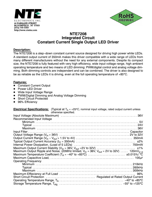
NTE7208Integrated CircuitConstant Current Single Output LED DriverDescription:The NTE7208 is a step-down constant current source designed for driving high power white LEDs.A standard output current of 350mA makes this driver compatible with a wide range of LEDs from many different manufacturers without the need for any external components. Despite its compact size, the NTE7208 is fully featured with very high efficiency, wide input voltage range, high ambient operating temperature and two means of LED dimming: PWM/digital control and analog voltage dim‐ming. Both dimming controls are independent and can be combined. The driver is also designed to be as reliable as the LEDs it is driving, even at the full operating temperature of +85°C.Features:D Constant Current OutputD Power LED DriverD Wide Input Voltage RangeD PWM/Digital Dimming and Analog Voltage DimmingD Short Circuit ProtectedD96% EfficiencyElectrical Specifications:(Typical at T A = +25°C, nominal input voltage, rated output current unlessotherwise specified.. . . . . . . . . . . . . . . . . . . . . . . . . . . . . . . . . . . . . . . . . . . . . . . . . . . Input Voltage (Absolute Maximum)36V Recommended Input Voltage. . . . . . . . . . . . . . . . . . . . . . . . . . . . . . . . . . . . . . . . . . . . . . . . . . . . . . . . . . . . . . . . . . . . .Minimum5V . . . . . . . . . . . . . . . . . . . . . . . . . . . . . . . . . . . . . . . . . . . . . . . . . . . . . . . . . . . . . . . . . . . . . .Typical24V Maximum36V . . . . . . . . . . . . . . . . . . . . . . . . . . . . . . . . . . . . . . . . . . . . . . . . . . . . . . . . . . . . . . . . . . .. . . . . . . . . . . . . . . . . . . . . . . . . . . . . . . . . . . . . . . . . . . . . . . . . . . . . . . . . . . . . . . . . . . .Input Filter Capacitor. . . . . . . . . . . . . . . . . . . . . . . . . . . . . . . . . . . . . . . . . . . . . . .Output Voltage Range (V in= 36V)2V to 32V. . . . . . . . . . . . . . . . . . . . . . . . . . . . . . . . . . . . . . Output Current Range (V in - V out> 1.5V to 4V)350mA. . . . . . . . . . . . . . . . . . . . . . . . . . . . . . . . . . . . . . . . Typical Output Current Accuracy (I O = 350mA)±2%. . . . . . . . . . . . . . . . . . . . . . . . . . . . . . . . . . . . . . Internal Power Dissipation, (Load of 5 LEDs)700mW. . . . . . . . . . . . . . . . . . . . . . . . . . Maximum Output Current Stability (V in = 36V, V out =2V to 32V)±1%. . . . . Maximum Output Ripple and Noise, (20MHz limited, V in = 36V, V out = 2V to 32V)120mV p-p. . . . . . . . . . . . . . . . . . . . . . . . .Maximum Temperature Coefficient (T A = -40° to +85°C)±0.015%/ °C. . . . . . . . . . . . . . . . . . . . . . . . . . . . . . . . . . . . . . . . . . . . . . . . . . . . . . . . Maximum Capacitive Load,100μF Operating Frequency. . . . . . . . . . . . . . . . . . . . . . . . . . . . . . . . . . . . . . . . . . . . . . . . . . . . . . . . . . . . . . . . .Minimum210kHz . . . . . . . . . . . . . . . . . . . . . . . . . . . . . . . . . . . . . . . . . . . . . . . . . . . . . . . . . . . . . . . . . . .Typical260kHz . . . . . . . . . . . . . . . . . . . . . . . . . . . . . . . . . . . . . . . . . . . . . . . . . . . . . . . . . . . . . . . .Maximum300kHz. . . . . . . . . . . . . . . . . . . . . . . . . . . . . . . . . . . . . . . . . . . . . . . . . . . Maximum Effieciency at Full Load96%. . . . . . . . . . . . . . . . . . . . . . . . . . . . . . . . .Short Circuit Protection Regulated at Rated Output Current. . . . . . . . . . . . . . . . . . . . . . . . . . . . . . . . . . . . . . . . . . .Operating Temperature Range, T A-40° to +85°C. . . . . . . . . . . . . . . . . . . . . . . . . . . . . . . . . . . . . . . . . .Storage Temperature Range, T stg-55° to +125°CElectrical Specifications (Cont'd):(Typical at T A = +25°C, nominal input voltage, rated output currentunless otherwise specified.. . . . . . . . . . . . . . . . . . . . . . . . . . . . . . . . . . . . . . . . . . . . . . . . . . Maximum Case Tempeature, T C+100°C. . . . . . . . . . . . . . . . . . . . . . . . . . . . . . . . . . . . . . . . .Thermal Impedance (Nature Convection)+55°C/W . . . . . . . . . . . . . . . . . . . . . . . . . . . . . . . . . . . . . . . . . . . . . . .Case Material Non Conductive Black Plastic Potting Material Epoxy (UL94-V0) . . . . . . . . . . . . . . . . . . . . . . . . . . . . . . . . . . . . . . . . . . . . . . . . . . . . . . . .. . . . . . . . . . . . . . . . . . . . . . . . . . . . . . . . . . . . . Maximum Wave Soldering Profile (10 seconds)+235°C PWM Dimming and ON/OFF Control (Leave Open if Not Used):Remote ON/OFFDC/DC ON,Open or 0V < V r < 0.6V . . . . . . . . . . . . . . . . . . . . . . . . . . . . . . . . . . . . . . . . . . . . . . . . .. . . . . . . . . . . . . . . . . . . . . . . . . . . . . . . . . . . . . . . . . . . . . .DC/DC OFF (Standby)0.6 < V r < 2.9V. . . . . . . . . . . . . . . . . . . . . . . . . . . . . . . . . . . . . . . . . . . . . .DC/DC OFF (Shutdown), 2.9 < V r < 6V. . . . . . . . . . . . . . . . . . . . . . . . . . . . . . . . . . . . . . . . Maximum Remote Pin Drive Current (V r = 5V)1mA Maximum Quiescent Input Current in Shutdown Mode (V in = 36V, V r > 2.9V)200μA. . . . . . . . . . . .. . . . . . . Maximum PWM Frequency for Linear Operation (measured 10% to 90% Dimming)200Hz Analog Dimming Control (Leave Open if Not Used):. . . . . . . . . . . . . . . . . . . . . . . . . . . . . . . . . . . . . . . . . . . . . . . . . . . . . . . . . . . .Input Voltage Range0 to 15V Control Voltage Range Limits. . . . . . . . . . . . . . . . . . . . . . . . . . . . . . . . . . . . . . . . . . . . . . . . . . . . . . . . . . . . .Full On0.13V ± 50mV . . . . . . . . . . . . . . . . . . . . . . . . . . . . . . . . . . . . . . . . . . . . . . . . . . . . . . . . . . . . . .Full Off 4.5V ± 50mV. . . . . . . . . . . . . . . . . . . . . . . . . . . . . . . . . . . . . . . . Maximum Analog Pin Drive Current (V c = 5V)0.2mA Environmental:. . . . . . . . . . . . . . . . . . . . . . . . . . . . . .Relative Humidity (See Note)5% to 95% RH, non-condensing . . . . . . . . . . . . . . . . . . . . . . . . . . . . . . . . . . . . . . . . . . . . . . . . . .Conducted Emissions EN55022, Class B . . . . . . . . . . . . . . . . . . . . . . . . . . . . . . . . . . . . . . . . . . . . . . . . . . .Radiated Emissions EN55022, Class B . . . . . . . . . . . . . . . . . . . . . . . . . . . . . . . . . . . . . . . . . . . . . . . . . . . . . . . . . . . . .ESD EN61000-4-2, Class A . . . . . . . . . . . . . . . . . . . . . . . . . . . . . . . . . . . . . . . . . . . . . . . .Radiated Immunity EN61000-4-3, Class A Fast Transient EN61000-4-4, Class A . . . . . . . . . . . . . . . . . . . . . . . . . . . . . . . . . . . . . . . . . . . . . . . . . . . .. . . . . . . . . . . . . . . . . . . . . . . . . . . . . . . . . . . . . . . . . . . . . . .Conducted Immunity EN61000-4-6, Class A MTBF (RCD-24-0.70, Nominal V in, Full Load)+25°C605 x 103 hours . . . . . . . . . . . . . . . . . . . . . . . . . . . . . . . . . . . . . . . . . . . . . . . . . . . . . . . . . . . .. . . . . . . . . . . . . . . . . . . . . . . . . . . . . . . . . . . . . . .Using MIL-HDBK 217F, +71°C516 x 103 hoursNote: Requires an input filter to meet EN55022 Class B conducted emissions, see below.。
Binomial coefficient
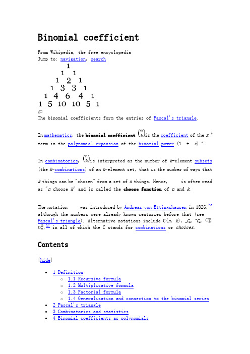
Binomial coefficientFrom Wikipedia, the free encyclopediaJump to: navigation, searchThe binomial coefficients form the entries of Pascal's triangle.In mathematics, the binomial coefficient is the coefficient of the x k term in the polynomial expansion of the binomial power (1 + x)n.In combinatorics, is interpreted as the number of k-element subsets (the k-combinations) of an n-element set, that is the number of ways thatk things can be "chosen" from a set of n things. Hence, is often read as "n choose k" and is called the choose function of n and k.The notation was introduced by Andreas von Ettingshausen in 1826,[1] although the numbers were already known centuries before that (seePascal's triangle). Alternative notations include C(n, k), n C k, n C k,,[2] in all of which the C stands for combinations or choices.Contents[hide]∙ 1 Definitiono 1.1 Recursive formulao 1.2 Multiplicative formulao 1.3 Factorial formulao 1.4 Generalization and connection to the binomial series ∙ 2 Pascal's triangle∙ 3 Combinatorics and statistics∙ 4 Binomial coefficients as polynomialso 4.1 Binomial coefficients as a basis for the space of polynomialso 4.2 Integer-valued polynomialso 4.3 Example∙ 5 Identities involving binomial coefficientso 5.1 Powers of -1o 5.2 Series involving binomial coefficientso 5.3 Identities with combinatorial proofso 5.4 Continuous identities∙ 6 Generating functionso 6.1 Ordinary generating functions∙7 Divisibility properties∙8 Bounds and asymptotic formulas∙9 Generalizationso9.1 Generalization to multinomialso9.2 Generalization to negative integerso9.3 Taylor serieso9.4 Binomial coefficient with n=1/2o9.5 Identity for the product of binomial coefficientso9.6 Partial Fraction Decompositiono9.7 Newton's binomial serieso9.8 Two real or complex valued argumentso9.9 Generalization to q-serieso9.10 Generalization to infinite cardinals∙10 Binomial coefficient in programming languages∙11 See also∙12 Notes∙13 References[edit] DefinitionFor natural numbers(taken to include 0) n and k, the binomial coefficientcan be defined as the coefficient of the monomial X k in the expansion of (1 + X)n. The same coefficient also occurs (if k≤ n) in the binomial formula(valid for any elements x,y of a commutative ring), which explains the name "binomial coefficient".Another occurrence of this number is in combinatorics, where it gives the number of ways, disregarding order, that a k objects can be chosen from among n objects; more formally, the number of k-element subsets (ork-combinations) of an n-element set. This number can be seen to be equal to the one of the first definition, independently of any of the formulas below to compute it: if in each of the n factors of the power (1 + X)n one temporarily labels the term X with an index i(running from 1 to n), then each subset of k indices gives after expansion a contribution X k, and the coefficient of that monomial in the result will be the number ofsuch subsets. This shows in particular that is a natural number for any natural numbers n and k. There are many other combinatorial interpretations of binomial coefficients (counting problems for which the answer is given by a binomial coefficient expression), for instance the number of words formed of n bits(digits 0 or 1) whose sum is k, but most of these are easily seen to be equivalent to counting k-combinations.Several methods exist to compute the value of without actually expanding a binomial power or counting k-combinations.[edit] Recursive formulaOne has a recursive formula for binomial coefficientswith as initial valuesThe formula follows either from tracing the contributions to X k in (1 + X)n−1(1 + X), or by counting k-combinations of {1, 2, ..., n} that containn and that do not contain n separately. It follows easily thatwhen k > n, and for all n, so the recursion can stop when reaching such cases. This recursive formula then allows the construction of Pascal's triangle.[edit] Multiplicative formulaA more efficient method to compute individual binomial coefficients is given by the formulaThis formula is easiest to understand for the combinatorial interpretation of binomial coefficients. The numerator gives the number of ways to select a sequence of k distinct objects, retaining the order of selection, from a set of n objects. The denominator counts the number of distinct sequences that define the same k-combination when order is disregarded.[edit] Factorial formulaFinally there is a formula using factorials that is easy to remember:where n! denotes the factorial of n. This formula follows from the multiplicative formula above by multiplying numerator and denominator by (n−k)!; as a consequence it involves many factors common to numerator and denominator. It is less practical for explicit computation unless common factors are first canceled (in particular since factorial values grow very rapidly). The formula does exhibit a symmetry that is less evident from the multiplicative formula (though it is from the definitions)[edit] Generalization and connection to the binomial seriesThe multiplicative formula allows the definition of binomial coefficients to be extended[note 1] by replacing n by an arbitrary number α (negative, real, complex) or even an element of any commutative ring in which all positive integers are invertible:With this definition one has a generalization of the binomial formula (with one of the variables set to 1), which justifies still calling thebinomial coefficients:This formula is valid for all complex numbers α and X with |X| < 1. It can also be interpreted as an identity of formal power series in X, where it actually can serve as definition of arbitrary powers of series with constant coefficient equal to 1; the point is that with this definition all identities hold that one expects for exponentiation, notablyIf αis a nonnegative integer n, then all terms with k > n are zero, and the infinite series becomes a finite sum, thereby recovering the binomial formula. However for other values of α, including negative integers and rational numbers, the series is really infinite.[edit] Pascal's triangleMain article: Pascal's ruleMain article: Pascal's trianglePascal's rule is the important recurrence relationwhich can be used to prove by mathematical induction that is a natural number for all n and k, (equivalent to the statement that k! divides the product of k consecutive integers), a fact that is not immediately obvious from formula (1).Pascal's rule also gives rise to Pascal's triangle:0: 11: 1 12: 1 2 13: 1 3 3 14: 1 4 6 4 15: 1 5 10 10 5 16: 1 6 15 20 15 6 17: 1 7 21 35 35 21 7 18: 1 8 28 56 70 56 28 8 1Row number n contains the numbers for k= 0,…,n. It is constructed by starting with ones at the outside and then always adding two adjacent numbers and writing the sum directly underneath. This method allows the quick calculation of binomial coefficients without the need for fractions or multiplications. For instance, by looking at row number 5 of the triangle, one can quickly read off that(x + y)5 = 1x5 + 5x4y + 10x3y2 + 10x2y3 + 5x y4 + 1y5.The differences between elements on other diagonals are the elements in the previous diagonal, as a consequence of the recurrence relation (3) above.[edit] Combinatorics and statisticsBinomial coefficients are of importance in combinatorics, because they provide ready formulas for certain frequent counting problems:There are ways to choose k elements from a set of n elements.See Combination.∙There are ways to choose k elements from a set of n if repetitions are allowed. See Multiset.∙There are strings containing k ones and n zeros.∙There are strings consisting of k ones and n zeros such that no two ones are adjacent.∙The Catalan numbers are∙The binomial distribution in statistics is∙The formula for a Bézier curve.[edit] Binomial coefficients as polynomialsFor any nonnegative integer k, the expression can be simplified and defined as a polynomial divided by k!:This presents a polynomial in t with rational coefficients.As such, it can be evaluated at any real or complex number t to define binomial coefficients with such first arguments. These "generalized binomial coefficients" appear in Newton's generalized binomial theorem.For each k, the polynomial can be characterized as the unique degree k polynomial p(t) satisfying p(0) = p(1) = ... = p(k− 1) = 0 and p(k) = 1.Its coefficients are expressible in terms of Stirling numbers of the first kind, by definition of the latter:The derivative of can be calculated by logarithmic differentiation:[edit] Binomial coefficients as a basis for the space of polynomialsOver any field containing Q, each polynomial p(t) of degree at most d isuniquely expressible as a linear combination . The coefficient a k is the k th difference of the sequence p(0), p(1), …, p(k). Explicitly,[note 2][edit] Integer-valued polynomialsEach polynomial is integer-valued: it takes integer values at integer inputs. (One way to prove this is by induction on k, using Pascal's identity.) Therefore any integer linear combination of binomial coefficient polynomials is integer-valued too. Conversely, (3.5) shows that any integer-valued polynomial is an integer linear combination of these binomial coefficient polynomials. More generally, for any subring R of a characteristic 0 field K, a polynomial in K[t] takes values in R at all integers if and only if it is an R-linear combination of binomial coefficient polynomials.[edit] ExampleThe integer-valued polynomial 3t(3t + 1)/2 can be rewritten as[edit] Identities involving binomial coefficientsFor any nonnegative integers n and k,This follows from (2) by using (1 + x)n = x n·(1 + x−1)n. It is reflected in the symmetry of Pascal's triangle. A combinatorial interpretation of this formula is as follows: when forming a subset of k elements (from a set of size n), it is equivalent to consider the number of ways you can pick k elements and the number of ways you can exclude n−k elements. The factorial definition lets one relate nearby binomial coefficients. For instance, if k is a positive integer and n is arbitrary, thenand, with a little more work,[edit] Powers of -1A special binomial coefficient is ; it equals powers of -1:[edit] Series involving binomial coefficientsThe formulais obtained from (2) using x = 1. This is equivalent to saying that the elements in one row of Pascal's triangle always add up to two raised to an integer power. A combinatorial interpretation of this fact involving double counting is given by counting subsets of size 0, size 1, size 2, and so on up to size n of a set S of n elements. Since we count the number of subsets of size i for 0 ≤ i≤ n, this sum must be equal to the number of subsets of S, which is known to be 2n. That is, Equation 5 is a statement that the power set for a finite set with n elements has size 2n.The formulasandfollow from (2), after differentiating with respect to x (twice in the latter) and then substituting x = 1.Vandermonde's identityis found by expanding (1 + x)m (1 + x)n−m = (1 + x)n with (2). As is zero if k > n, the sum is finite for integer n and m. Equation (7a) generalizes equation (3). It holds for arbitrary, complex-valued m and n, the Chu-Vandermonde identity.A related formula isWhile equation (7a) is true for all values of m, equation (7b) is true for all values of j between 0 and k inclusive.From expansion (7a) using n=2m, k = m, and (4), one findsLet F(n) denote the n th Fibonacci number. We obtain a formula about the diagonals of Pascal's triangleThis can be proved by induction using (3) or by Zeckendorf's representation (Just note that the lhs gives the number of subsets of {F(2),...,F(n)} without consecutive members, which also form all the numbers below F(n+1)).Also using (3) and induction, one can show thatAgain by (3) and induction, one can show that for k = 0, ... , n−1as well aswhich is itself a special case of the result from the theory of finite differences that for any polynomial P(x) of degree less than n,[citation needed]Differentiating (2) k times and setting x = −1 yields this for, when 0 ≤ k< n, and the general case follows by taking linear combinations of these.When P(x) is of degree less than or equal to n,where a n is the coefficient of degree n in P(x).More generally for 13b,where m and d are complex numbers. This follows immediately applying (13b) to the polynomial Q(x):=P(m + dx)instead of P(x), and observing that Q(x) has still degree less than or equal to n, and that its coefficient of degree n is d n a n.The infinite seriesis convergent for k≥ 2. This formula is used in the analysis of the German tank problem. It is equivalent to the formula for the finite sumwhich is proved for M>m by induction on M.Using (8) one can deriveand.[edit] Identities with combinatorial proofsMany identities involving binomial coefficients can be proved by combinatorial means. For example, the following identity for nonnegativeintegers (which reduces to (6) when q = 1):can be given a double counting proof as follows. The left side counts the number of ways of selecting a subset of [n] of at least q elements, and marking q elements among those selected. The right side counts the same parameter, because there are ways of choosing a set of q marks and they occur in all subsets that additionally contain some subset of the remaining elements, of which there are 2n−q.The recursion formulawhere both sides count the number of k-element subsets of {1, 2, . . . , n} with the right hand side first grouping them into those which contain element n and those which don’t.The identity (8) also has a combinatorial proof. The identity readsSuppose you have 2n empty squares arranged in a row and you want to mark(select) n of them. There are ways to do this. On the other hand, you may select your n squares by selecting k squares from among the first n and n−k squares from the remaining n squares. This givesNow apply (4) to get the result.[edit] Continuous identitiesCertain trigonometric integrals have values expressible in terms of binomial coefficients:For andThese can be proved by using Euler's formula to convert trigonometric functions to complex exponentials, expanding using the binomial theorem, and integrating term by term.[edit] Generating functions[edit] Ordinary generating functionsFor a fixed n, the ordinary generating function of the sequenceis:For a fixed k, the ordinary generating function of the sequenceis:The bivariate generating function of the binomial coefficients is:[edit] Divisibility propertiesIn 1852, Kummer proved that if m and n are nonnegative integers and p isa prime number, then the largest power of p dividing equals p c, where c is the number of carries when m and n are added in base p. Equivalently,the exponent of a prime p in equals the number of positive integers j such that the fractional part of k/p j is greater than the fractionalpart of n/p j. It can be deduced from this that is divisible byn/gcd(n,k).A somewhat surprising result by David Singmaster (1974) is that any integer divides almost all binomial coefficients. More precisely, fix aninteger d and let f(N) denote the number of binomial coefficientswith n < N such that d divides . ThenSince the number of binomial coefficients with n < N is N(N+1) / 2, this implies that the density of binomial coefficients divisible by d goes to 1.Another fact: An integer n≥ 2 is prime if and only if all the intermediate binomial coefficientsare divisible by n.Proof: When p is prime, p dividesfor all 0 < k < pbecause it is a natural number and the numerator has a prime factor p but the denominator does not have a prime factor p.When n is composite, let p be the smallest prime factor of n and let k = n/p. Then 0 < p < n andotherwise the numerator k(n−1)(n−2)×...×(n−p+1) has to be divisible by n = k×p, this can only be the case when (n−1)(n−2)×...×(n−p+1) is divisible by p. But n is divisible by p, so p does not divide n−1, n−2, ..., n−p+1 and because p is prime, we know that p does not divide(n−1)(n−2)×...×(n−p+1) and so the numerator cannot be divisible by n. [edit] Bounds and asymptotic formulasThe following bounds for hold:Stirling's approximation yields the bounds:and, in general,for m≥ 2 and n≥ 1,and the approximationasThe infinite product formula (cf. Gamma function, alternative definition)yields the asymptotic formulasas .This asymptotic behaviour is contained in the approximationas well. (Here H k is the k th harmonic number and γis the Euler–Mascheroni constant).The sum of binomial coefficients can be bounded by a term exponential in n and the binary entropy of the largest n/ k that occurs. More precisely,for and , it holdswhere is the binary entropy of ε.[3]A simple and rough upper bound for the sum of binomial coefficients is given by the formula below (not difficult to prove)[edit] Generalizations[edit] Generalization to multinomialsBinomial coefficients can be generalized to multinomial coefficients. They are defined to be the number:whereWhile the binomial coefficients represent the coefficients of (x+y)n, the multinomial coefficients represent the coefficients of the polynomialSee multinomial theorem. The case r = 2 gives binomial coefficients:The combinatorial interpretation of multinomial coefficients is distribution of n distinguishable elements over r (distinguishable) containers, each containing exactly k i elements, where i is the index of the container.Multinomial coefficients have many properties similar to these of binomial coefficients, for example the recurrence relation:and symmetry:where (σi) is a permutation of (1,2,...,r).[edit] Generalization to negative integersIf , thenextends to all n.[edit] Taylor seriesUsing Stirling numbers of the first kind the series expansion around any arbitrarily chosen point z0 is[edit] Binomial coefficient with n=1/2The definition of the binomial coefficients can be extended to the case where n is real and k is integer.In particular, the following identity holds for any non-negative integer k :This shows up when expanding into a power series using the Newtonbinomial series :[edit] Identity for the product of binomial coefficientsOne can express the product of binomial coefficients as a linear combination of binomial coefficients:where the connection coefficients are multinomial coefficients. In terms of labelled combinatorial objects, the connection coefficients represent the number of ways to assign m+n-k labels to a pair of labelled combinatorial objects of weight m and n respectively, that have had their first k labels identified, or glued together, in order to get a new labelled combinatorial object of weight m+n-k. (That is, to separate the labels into 3 portions to be applied to the glued part, the unglued part of the first object, and the unglued part of the second object.) In this regard, binomial coefficients are to exponential generating series what falling factorials are to ordinary generating series.[edit] Partial Fraction DecompositionThe partial fraction decomposition of the inverse is given byand[edit] Newton's binomial seriesNewton's binomial series, named after Sir Isaac Newton, is one of the simplest Newton series:The identity can be obtained by showing that both sides satisfy the differential equation (1+z) f'(z) = αf(z).The radius of convergence of this series is 1. An alternative expression iswhere the identityis applied.[edit] Two real or complex valued argumentsThe binomial coefficient is generalized to two real or complex valued arguments using the gamma function or beta function viaThis definition inherits these following additional properties from Γ:moreover,The resulting function has been little-studied, apparently first being graphed in (Fowler 1996). Notably, many binomial identities fail:but for n positive (so −n negative). The behavior is quite complex, and markedly different in various octants (that is, with respect to the x and y axes and the line y= x), with the behavior for negative x having singularities at negative integer values and a checkerboard of positive and negative regions:∙in the octant it is a smoothly interpolated form of the usual binomial, with a ridge ("Pascal's ridge").∙in the octant and in the quadrant the function is close to zero.∙in the quadrant the function is alternatingly very large positive and negative on the parallelograms with vertices ( −n,m + 1),( −n,m),( −n− 1,m− 1),( −n− 1,m) ∙in the octant 0 > x > y the behavior is again alternatingly very large positive and negative, but on a square grid.∙in the octant − 1 > y > x + 1 it is close to zero, except for near the singularities.[edit] Generalization to q-seriesThe binomial coefficient has a q-analog generalization known as the Gaussian binomial coefficient.[edit] Generalization to infinite cardinalsThe definition of the binomial coefficient can be generalized to infinite cardinals by defining:where A is some set with cardinalityα. One can show that the generalized binomial coefficient is well-defined, in the sense that no matter whatset we choose to represent the cardinal number α, will remain the same. For finite cardinals, this definition coincides with the standard definition of the binomial coefficient.Assuming the Axiom of Choice, one can show that for any infinite cardinal α.[edit] Binomial coefficient in programming languagesThe notation is convenient in handwriting but inconvenient for typewriters and computer terminals. Many programming languages do not offer a standard subroutine for computing the binomial coefficient, but for example the J programming language uses the exclamation mark: k ! n .Naive implementations of the factorial formula, such as the following snippet in C:int choose(int n, int k) {return factorial(n) / (factorial(k) * factorial(n - k));}are prone to overflow errors, severely restricting the range of input values. A direct implementation of the multiplicative formula works well:unsigned long long choose(unsigned n, unsigned k) {if (k > n)return 0;if (k > n/2)k = n-k; // Take advantage of symmetrylong double accum = 1;unsigned i;for (i = 1; i <= k; i++)accum = accum * (n-k+i) / i;return accum + 0.5; // avoid rounding error}Another way to compute the binomial coefficient when using large numbers is to recognize thatlnΓ(n) is a special function that is easily computed and is standard in some programming languages such as using log_gamma in Maxima, LogGamma in Mathematica, or gammaln in MATLAB. Roundoff error may cause the returned value not to be an integer.[edit] See also∙Central binomial coefficient∙Binomial transform∙Star of David theorem∙Table of Newtonian series∙List of factorial and binomial topics∙Multiplicities of entries in Pascal's triangle∙Sun's curious identity[edit] Notes1.^See (Graham, Knuth & Patashnik 1994), which also defines fork< 0. Alternative generalizations, such as to two real or complex valued arguments using the Gamma function assign nonzero values tofor k< 0, but this causes most binomial coefficient identities to fail, and thus is not widely used majority of definitions. Onesuch choice of nonzero values leads to the aesthetically pleasing "Pascal windmill" in Hilton, Holton and Pedersen, Mathematicalreflections: in a room with many mirrors, Springer, 1997, but causes even Pascal's identity to fail (at the origin).2.^This can be seen as a discrete analog of Taylor's theorem. It isclosely related to Newton's polynomial. Alternating sums of this form may be expressed as the Nörlund–Rice integral.[edit] References1.^Nicholas J. Higham. Handbook of writing for the mathematicalsciences. SIAM. p. 25. ISBN0898714206.2.^ G. E. Shilov (1977). Linear algebra. Dover Publications.ISBN9780486635187.3.^ see e.g. Flum & Grohe (2006, p. 427)∙Fowler, David(January 1996). "The Binomial Coefficient Function".The American Mathematical Monthly(Mathematical Association ofAmerica) 103 (1): 1–17. doi:10.2307/2975209./stable/2975209∙Knuth, Donald E.(1997). The Art of Computer Programming, Volume 1: Fundamental Algorithms (Third ed.). Addison-Wesley.pp. 52–74. ISBN0-201-89683-4.∙Graham, Ronald L.; Knuth, Donald E.; Patashnik, Oren (1994).Concrete Mathematics (Second ed.). Addison-Wesley.pp. 153–256. ISBN0-201-55802-5.∙Singmaster, David (1974). "Notes on binomial coefficients. III.Any integer divides almost all binomial coefficients". J. LondonMath. Soc. (2)8: 555–560. doi:10.1112/jlms/s2-8.3.555.∙Bryant, Victor (1993). Aspects of combinatorics. Cambridge University Press.∙Arthur T. Benjamin; Jennifer Quinn, Proofs that Really Count: The Art of Combinatorial Proof, Mathematical Association of America,2003.∙Flum, Jörg; Grohe, Martin (2006). Parameterized Complexity Theory.Springer. ISBN978-3-540-29952-3./east/home/generic/search/results?SGWID=5-40109-22-141358322-0.This article incorporates material from the following PlanetMath articles, which are licensed under the Creative Commons Attribution/Share-Alike License: Binomial Coefficient, Bounds for binomial coefficients, Proof that C(n,k) is an integer, Generalized binomial coefficients.。
Stirling Engine Plans 斯特林发动机模型简易图纸
\」回3132'
斗护/泣T
回::J '
③
I
3 /3 2' To p 7M
E:>f MC 25i叫
⑩
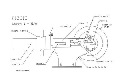
FIZGIG
Shee 吃
12
Li gh 吃 weigh 吃
Pis 吃 on ,
'-'μ r ~ ~
@口
2
311 坦
>SSU E' 0 (B E'-t oJ
C C>n俨。d
M龟 w e e n
c e ntr e ~
Sheet 7
Cylinde 俨&
豆二
Pis 吃 on
@口
(8" 变 α 〉
37/6 ~
"♂
E
Lodite ω〉唁
( tetedr T
~-- Approx
See de~ωled no 飞 E for fit协 9 p'" 毛~ to cy们 nder
@
一一γ
→忖←
U~
'"
也旬'
白
S .,..,. Sh ee t II for
"' r . QOk . d
"" hol. . T Ip of 1/驴
, .啊<co肝脏 l
《 ?①
},
,-,
E
g
E:>, ~c …
FIZGIG
Issue 0
4
Sheet 2b (Be 吃 Q)
1110' or 2MN bedplQte 0 口
S ~ ve 俨 5old~r
3/1豆
IEC vibration test standard
* * Voir adresse «site web» sur la page de titre.
See web site address on title page.
NORME INTERNATIONALE INTERNATIONAL STANDARD
CEI IEC 60068-2-57
Deuxième édition Second edition 1999-11
Numéro de référence Reference number CEI/IEC 60068-2ications
Depuis le 1er janvier 1997, les publications de la CEI sont numérotées à partir de 60000.
•
•
Terminologie, symboles graphiques et littéraux
En ce qui concerne la terminologie générale, le lecteur se reportera à la CEI 60050: Vocabulaire Electrotechnique International (VEI). Pour les symboles graphiques, les symboles littéraux et les signes d'usage général approuvés par la CEI, le lecteur consultera la CEI 60027: Symboles littéraux à utiliser en électrotechnique, la CEI 60417: S ymboles graphiques utilisables sur le matériel. Index, relevé et compilation des feuilles individuelles, et la CEI 60617: Symboles graphiques pour schémas.
POJ题目分类
1000 A+B Problem 送分题1001 Exponentiation 高精度1003 Hangover 送分题1004 Financial Management 送分题1005 I Think I Need a Houseboat 几何1006 Biorhythms 送分题1007 DNA Sorting 送分题1008 Maya Calendar 日期处理1010 STAMPS 搜索+DP1011 Sticks 搜索1012 Joseph 模拟/数学方法1014 Dividing 数论/DP?/组合数学->母函数?1015 Jury Compromise DP1016 Numbers That Count 送分题1017 Packets 贪心1018 Communication System 贪心1019 Number Sequence 送分题1020 Anniversary Cake 搜索1023 The Fun Number System 数论1025 Department 模拟1026 Cipher 组合数学1027 The Same Game 模拟1028 Web Navigation 送分题1031 Fence 计算几何1034 The dog task 计算几何1037 A decorative fence DP/组合数学1039 Pipe 几何1042 Gone Fishing 贪心/DP1045 Bode Plot 送分题(用物理知识)1046 Color Me Less 送分题1047 Round and Round We Go 高精度1048 Follow My Logic 模拟1049 Microprocessor Simulation 模拟1050 To the Max DP1053 Set Me 送分题1054 The Troublesome Frog 搜索1060 Modular multiplication of polynomials 高精度1061 青蛙的约会数论1062 昂贵的聘礼DP1064 Cable master DP/二分查找1065 Wooden Sticks DP1067 取石子游戏博弈论1068 Parencodings 送分题1069 The Bermuda Triangle 搜索1070 Deformed Wheel 几何1071 Illusive Chase 送分题1072 Puzzle Out 搜索1073 The Willy Memorial Program 模拟1074 Parallel Expectations DP1075 University Entrance Examination 模拟1080 Human Gene Functions DP->LCS变形1082 Calendar Game 博弈论1084 Square Destroyer 搜索?1085 Triangle War 博弈论1086 Unscrambling Images 模拟?1087 A Plug for UNIX 图论->最大流1088 滑雪DFS/DP1090 Chain ->格雷码和二进制码的转换1091 跳蚤数论1092 Farmland 几何1093 Formatting Text DP1094 Sorting It All Out 图论->拓扑排序1095 Trees Made to Order 组合数学1096 Space Station Shielding 送分题1097 Roads Scholar 图论1098 Robots 模拟1099 Square Ice 送分题1100 Dreisam Equations 搜索1101 The Game 搜索->BFS1102 LC-Display 送分题1103 Maze 模拟1104 Robbery 递推1106 Transmitters 几何1107 W's Cipher 送分题1110 Double Vision 搜索1111 Image Perimeters 搜索1112 Team Them Up! DP1113 Wall 计算几何->convex hull1119 Start Up the Startup 送分题1120 A New Growth Industry 模拟1122 FDNY to the Rescue! 图论->Dijkstra 1125 Stockbroker Grapevine 图论->Dijkstra 1128 Frame Stacking 搜索1129 Channel Allocation 搜索(图的最大独立集)1131 Octal Fractions 高精度1135 Domino Effect 图论->Dijkstra1137 The New Villa 搜索->BFS1141 Brackets Sequence DP1142 Smith Numbers 搜索1143 Number Game 博弈论1147 Binary codes 构造1148 Utopia Divided 构造1149 PIGS 图论->网络流1151 Atlantis 计算几何->同等安置矩形的并的面积->离散化1152 An Easy Problem! 数论1157 LITTLE SHOP OF FLOWERS DP1158 TRAFFIC LIGHTS 图论->Dijkstra变形1159 Palindrome DP->LCS1160 Post Office DP1161 Walls 图论1162 Building with Blocks 搜索1163 The Triangle DP1170 Shopping Offers DP1177 Picture 计算几何->同等安置矩形的并的周长->线段树1179 Polygon DP1180 Batch Scheduling DP1182 食物链数据结构->并查集1183 反正切函数的应用搜索1184 聪明的打字员搜索1185 炮兵阵地DP->数据压缩1187 陨石的秘密DP(BalkanOI99 Par的拓展)1189 钉子和小球递推?1190 生日蛋糕搜索/DP1191 棋盘分割DP1192 最优连通子集图论->无负权回路的有向图的最长路->BellmanFord 1193 内存分配模拟1194 HIDDEN CODES 搜索+DP1197 Depot 数据结构->Young T ableau1201 Intervals 贪心/图论->最长路->差分约束系统1202 Family 高精度1209 Calendar 日期处理1217 FOUR QUARTERS 递推1218 THE DRUNK JAILER 送分题1233 Street Crossing 搜索->BFS1245 Programmer, Rank Thyself 送分题1247 Magnificent Meatballs 送分题1248 Safecracker 搜索1250 T anning Salon 送分题1251 Jungle Roads 图论->最小生成树1271 Nice Milk 计算几何1273 Drainage Ditches 图论->最大流1274 The Perfect Stall 图论->二分图的最大匹配1275 Cashier Employment 图论->差分约束系统->无负权回路的有向图的最长路->Bellman-Ford1280 Game 递推1281 MANAGER 模拟1286 Necklace of Beads 组合数学->Polya定理1288 Sly Number 数论->解模线性方程组1293 Duty Free Shop DP1298 The Hardest Problem Ever 送分题1316 Self Numbers 递推同Humble Number一样1322 Chocolate 递推/组合数学1323 Game Prediction 贪心1324 Holedox Moving BFS+压缩储存1325 Machine Schedule 图论->二分图的最大匹配1326 Mileage Bank 送分题1327 Moving Object Recognition 模拟?1328 Radar Installation 贪心(差分约束系统的特例)1338 Ugly Numbers 递推(有O(n)算法)1364 King 图论->无负权回路的有向图的最长路->BellmanFord1370 Gossiping (数论->模线性方程有无解的判断)+(图论->DFS)2184 Cow Exhibition DP2190 ISBN 送分题2191 Mersenne Composite Numbers 数论2192 Zipper DP->LCS变形2193 Lenny's Lucky Lotto Lists DP2194 Stacking Cylinders 几何2195 Going Home 图论->二分图的最大权匹配2196 Specialized Four-Digit Numbers 送分题2197 Jill's Tour Paths 图论->2199 Rate of Return 高精度2200 A Card Trick 模拟2210 Metric Time 日期处理2239 Selecting Courses 图论->二分图的最大匹配2243 Knight Moves 搜索->BFS2247 Humble Numbers 递推(最优O(n)算法)2253 Frogger 图论->Dijkstra变形(和1295是一样的)2254 Globetrotter 几何2261 France '98 递推2275 Flipping Pancake 构造2284 That Nice Euler Circuit 计算几何2289 Jamie's Contact Groups 图论->网络流?2291 Rotten Ropes 送分题2292 Optimal Keypad DP2299 Ultra-QuickSort 排序->归并排序2304 Combination Lock 送分题2309 BST 送分题2311 Cutting Game 博弈论2312 Battle City 搜索->BFS2314 POJ language 模拟2315 Football Game 几何2346 Lucky tickets 组合数学2351 Time Zones 时间处理2379 ACM Rank T able 模拟+排序2381 Random Gap 数论2385 Apple Catching DP(像NOI98“免费馅饼”)2388 Who's in the Middle 送分题(排序)2390 Bank Interest 送分题2395 Out of Hay 图论->Dijkstra变形2400 Supervisor, Supervisee 图论->二分图的最大权匹配?2403 Hay Points 送分题2409 Let it Bead 组合数学->Polya定理2416 Return of the Jedi 图论->2417 Discrete Logging 数论2418 Hardwood Species 二分查找2419 Forests 枚举2421 Constructing Roads 图论->最小生成树2423 The Parallel Challenge Ballgame 几何2424 Flo's Restaurant 数据结构->堆2425 A Chess Game 博弈论2426 Remainder BFS2430 Lazy Cows DP->数据压缩1375 Intervals 几何1379 Run Away 计算几何->1380 Equipment Box 几何1383 Labyrinth 图论->树的最长路1394 Railroad 图论->Dijkstra1395 Cog-Wheels 数学->解正系数的线性方程组1408 Fishnet 几何1411 Calling Extraterrestrial Intelligence Again 送分题1430 Binary Stirling Numbers 日期处理1431 Calendar of Maya 模拟1432 Decoding Morse Sequences DP1434 Fill the Cisterns! 计算几何->离散化/1445 Random number 数据结构->碓1447 Ambiguous Dates 日期处理1450 Gridland 图论(本来TSP问题是NP难的,但这个图比较特殊,由现成的构造方法)1458 Common Subsequence DP->LCS1459 Power Network 图论->最大流1462 Random Walk 模拟+解线性方程组1463 Strategic game 贪心1466 Girls and Boys 图论->n/a1469 COURSES 贪心1475 Pushing Boxes DP1476 Always On the Run 搜索->BFS1480 Optimal Programs 搜索->BFS1481 The Die Is Cast 送分题1482 It's not a Bug, It's a Feature! 搜索->BFS1483 Going in Circles on Alpha Centauri 模拟1484 Blowing Fuses 送分题1485 Fast Food DP(似乎就是ioi2000的postoffice)1486 Sorting Slides 图论->拓扑排序1505 Copying Books DP+二分查找1510 Hares and Foxes 数论1512 Keeps Going and Going and ... 模拟1513 Scheduling Lectures DP1514 Metal Cutting 几何1515 Street Directions 图论->把一个无向连通图改造成为有向强连通图1517 u Calculate e 送分题1518 Problem Bee 几何1519 Digital Roots 送分题(位数可能很大)1520 Scramble Sort 排序1547 Clay Bully 送分题1555 Polynomial Showdown 送分题(非常阴险)1563 The Snail 送分题1601 Pizza Anyone? 搜索1604 Just the Facts 送分题1605 Horse Shoe Scoring 几何1606 Jugs 数论/搜索1631 Bridging signals DP+二分查找1632 Vase collection 图论->最大完全图1633 Gladiators DP1634 Who's the boss? 排序1635 Subway tree systems 图论->不同表示法的二叉树判同1637 Sightseeing tour 图论->欧拉回路1638 A number game 博弈论1639 Picnic Planning 图论->1641 Rational Approximation 数论1646 Double Trouble 高精度1654 Area 几何1657 Distance on Chessboard 送分题1658 Eva's Problem 送分题1660 Princess FroG 构造1661 Help Jimmy DP1663 Number Steps 送分题1664 放苹果组合数学->递推1677 Girls' Day 送分题1688 Dolphin Pool 计算几何1690 (Your)((Term)((Project))) 送分题1691 Painting A Board 搜索/DP1692 Crossed Matchings DP1693 Counting Rectangles 几何1694 An Old Stone Game 博弈论?1695 Magazine Delivery 图论->1712 Flying Stars DP1713 Divide et unita 搜索1714 The Cave 搜索/DP1717 Dominoes DP1718 River Crossing DP1719 Shooting Contest 贪心1729 Jack and Jill 图论->1730 Perfect Pth Powers 数论1732 Phone numbers DP1734 Sightseeing trip 图论->Euler回路1738 An old Stone Game 博弈论?1741 Tree 博弈论?1745 Divisibility DP1751 Highways 图论->1752 Advertisement 贪心/图论->差分约束系统1753 Flip Game 搜索->BFS1755 Triathlon 计算几何?1770 Special Experiment 树形DP1771 Elevator Stopping Plan DP1772 New Go Game 构造?1773 Outernet 模拟1774 Fold Paper Strips 几何1775 Sum of Factorials 送分题1776 T ask Sequences DP1777 Vivian's Problem 数论1870 Bee Breeding 送分题1871 Bullet Hole 几何1872 A Dicey Problem BFS1873 The Fortified Forest 几何+回溯1874 Trade on Verweggistan DP1875 Robot 几何1876 The Letter Carrier's Rounds 模拟1877 Flooded! 数据结构->堆1879 Tempus et mobilius Time and motion 模拟+组合数学->Polya定理1882 Stamps 搜索+DP1883 Theseus and the Minotaur 模拟1887 Testing the CATCHER DP1889 Package Pricing DP1893 Monitoring Wheelchair Patients 模拟+几何1915 Knight Moves 搜索->BFS1916 Rat Attack 数据结构->?1936 All in All DP?1946 Cow Cycling DP1947 Rebuilding Roads 二分1985 Cow Marathon 图论->有向无环图的最长路1995 Raising Modulo Numbers 数论->大数的幂求余2049 Finding Nemo 图论->最短路2050 Searching the Web 模拟(需要高效实现)2051 Argus 送分题(最好用堆,不用也可以过)2054 Color a Tree 贪心2061 Pseudo-random Numbers 数论2080 Calendar 日期处理2082 Terrible Sets 分治/2083 Fractal 递归2084 Game of Connections 递推(不必高精度)2105 IP Address 送分题2115 C Looooops 数论->解模线性方程2136 Vertical Histogram 送分题2165 Gunman 计算几何2179 Inlay Cutters 枚举2181 Jumping Cows 递推2182 Lost Cows ->线段树/=============================================1370 Gossiping (数论->模线性方程有无解的判断)+(图论->DFS)1090 Chain ->格雷码和二进制码的转换2182 Lost Cows ->线段树/2426 Remainder BFS1872 A Dicey Problem BFS1324 Holedox Moving BFS+压缩储存1088 滑雪DFS/DP1015 Jury Compromise DP1050 To the Max DP1062 昂贵的聘礼DP1065 Wooden Sticks DP1074 Parallel Expectations DP1093 Formatting Text DP1112 Team Them Up! DP1141 Brackets Sequence DP1157 LITTLE SHOP OF FLOWERS DP1160 Post Office DP1163 The Triangle DP1170 Shopping Offers DP1179 Polygon DP1180 Batch Scheduling DP1191 棋盘分割DP1293 Duty Free Shop DP2184 Cow Exhibition DP2193 Lenny's Lucky Lotto Lists DP2292 Optimal Keypad DP1432 Decoding Morse Sequences DP1475 Pushing Boxes DP1513 Scheduling Lectures DP1633 Gladiators DP1661 Help Jimmy DP1692 Crossed Matchings DP1712 Flying Stars DP1717 Dominoes DP1718 River Crossing DP1732 Phone numbers DP1745 Divisibility DP1771 Elevator Stopping Plan DP1776 T ask Sequences DP1874 Trade on Verweggistan DP1887 Testing the CATCHER DP1889 Package Pricing DP1946 Cow Cycling DP1187 陨石的秘密DP(BalkanOI99 Par的拓展)1485 Fast Food DP(似乎就是ioi2000的postoffice) 2385 Apple Catching DP(像NOI98“免费馅饼”) 1064 Cable master DP/二分查找1037 A decorative fence DP/组合数学1936 All in All DP?1505 Copying Books DP+二分查找1631 Bridging signals DP+二分查找1159 Palindrome DP->LCS1458 Common Subsequence DP->LCS1080 Human Gene Functions DP->LCS变形2192 Zipper DP->LCS变形1185 炮兵阵地DP->数据压缩2430 Lazy Cows DP->数据压缩1067 取石子游戏博弈论1082 Calendar Game 博弈论1085 Triangle War 博弈论1143 Number Game 博弈论2311 Cutting Game 博弈论2425 A Chess Game 博弈论1638 A number game 博弈论1694 An Old Stone Game 博弈论?1738 An old Stone Game 博弈论?1741 Tree 博弈论?2083 Fractal 递归1104 Robbery 递推1217 FOUR QUARTERS 递推1280 Game 递推2261 France '98 递推2181 Jumping Cows 递推1316 Self Numbers 递推同Humble Number一样2084 Game of Connections 递推(不必高精度) 1338 Ugly Numbers 递推(有O(n)算法)2247 Humble Numbers 递推(最优O(n)算法)1322 Chocolate 递推/组合数学1189 钉子和小球递推?1947 Rebuilding Roads 二分2418 Hardwood Species 二分查找2082 Terrible Sets 分治/1001 Exponentiation 高精度1047 Round and Round We Go 高精度1060 Modular multiplication of polynomials 高精度1131 Octal Fractions 高精度1202 Family 高精度2199 Rate of Return 高精度1646 Double Trouble 高精度1147 Binary codes 构造1148 Utopia Divided 构造2275 Flipping Pancake 构造1660 Princess FroG 构造1772 New Go Game 构造?1005 I Think I Need a Houseboat 几何1039 Pipe 几何1070 Deformed Wheel 几何1092 Farmland 几何1106 Transmitters 几何2194 Stacking Cylinders 几何2254 Globetrotter 几何2315 Football Game 几何2423 The Parallel Challenge Ballgame 几何1375 Intervals 几何1380 Equipment Box 几何1408 Fishnet 几何1514 Metal Cutting 几何1518 Problem Bee 几何1605 Horse Shoe Scoring 几何1654 Area 几何1693 Counting Rectangles 几何1774 Fold Paper Strips 几何1871 Bullet Hole 几何1875 Robot 几何1873 The Fortified Forest 几何+回溯1031 Fence 计算几何1034 The dog task 计算几何1271 Nice Milk 计算几何2284 That Nice Euler Circuit 计算几何1688 Dolphin Pool 计算几何2165 Gunman 计算几何1755 Triathlon 计算几何?1379 Run Away 计算几何->1113 Wall 计算几何->convex hull1434 Fill the Cisterns! 计算几何->离散化/1151 Atlantis 计算几何->同等安置矩形的并的面积->离散化1177 Picture 计算几何->同等安置矩形的并的周长->线段树2419 Forests 枚举2179 Inlay Cutters 枚举1025 Department 模拟1027 The Same Game 模拟1048 Follow My Logic 模拟1049 Microprocessor Simulation 模拟1073 The Willy Memorial Program 模拟1075 University Entrance Examination 模拟1098 Robots 模拟1103 Maze 模拟1120 A New Growth Industry 模拟1193 内存分配模拟1281 MANAGER 模拟2200 A Card Trick 模拟2314 POJ language 模拟1431 Calendar of Maya 模拟1483 Going in Circles on Alpha Centauri 模拟1512 Keeps Going and Going and ... 模拟1773 Outernet 模拟1876 The Letter Carrier's Rounds 模拟1883 Theseus and the Minotaur 模拟2050 Searching the Web 模拟(需要高效实现)1012 Joseph 模拟/数学方法1086 Unscrambling Images 模拟?1327 Moving Object Recognition 模拟?1893 Monitoring Wheelchair Patients 模拟+几何1462 Random Walk 模拟+解线性方程组2379 ACM Rank T able 模拟+排序1879 Tempus et mobilius Time and motion 模拟+组合数学->Polya定理1520 Scramble Sort 排序1634 Who's the boss? 排序2299 Ultra-QuickSort 排序->归并排序1008 Maya Calendar 日期处理1209 Calendar 日期处理2210 Metric Time 日期处理1430 Binary Stirling Numbers 日期处理1447 Ambiguous Dates 日期处理2080 Calendar 日期处理2351 Time Zones 时间处理1770 Special Experiment 树形DP1916 Rat Attack 数据结构->?1197 Depot 数据结构->Young T ableau1182 食物链数据结构->并查集2424 Flo's Restaurant 数据结构->堆1877 Flooded! 数据结构->堆1445 Random number 数据结构->碓1023 The Fun Number System 数论1061 青蛙的约会数论1091 跳蚤数论1152 An Easy Problem! 数论2191 Mersenne Composite Numbers 数论2381 Random Gap 数论2417 Discrete Logging 数论1510 Hares and Foxes 数论1641 Rational Approximation 数论1730 Perfect Pth Powers 数论1777 Vivian's Problem 数论2061 Pseudo-random Numbers 数论1014 Dividing 数论/DP?/组合数学->母函数?1606 Jugs 数论/搜索1995 Raising Modulo Numbers 数论->大数的幂求余2115 C Looooops 数论->解模线性方程1288 Sly Number 数论->解模线性方程组1395 Cog-Wheels 数学->解正系数的线性方程组1000 A+B Problem 送分题1003 Hangover 送分题1004 Financial Management 送分题1006 Biorhythms 送分题1007 DNA Sorting 送分题1016 Numbers That Count 送分题1019 Number Sequence 送分题1028 Web Navigation 送分题1046 Color Me Less 送分题1053 Set Me 送分题1068 Parencodings 送分题1071 Illusive Chase 送分题1096 Space Station Shielding 送分题1099 Square Ice 送分题1102 LC-Display 送分题1107 W's Cipher 送分题1119 Start Up the Startup 送分题1218 THE DRUNK JAILER 送分题1245 Programmer, Rank Thyself 送分题1247 Magnificent Meatballs 送分题1250 T anning Salon 送分题1298 The Hardest Problem Ever 送分题1326 Mileage Bank 送分题2190 ISBN 送分题2196 Specialized Four-Digit Numbers 送分题2291 Rotten Ropes 送分题2304 Combination Lock 送分题2309 BST 送分题2390 Bank Interest 送分题2403 Hay Points 送分题1411 Calling Extraterrestrial Intelligence Again 送分题1481 The Die Is Cast 送分题1484 Blowing Fuses 送分题1517 u Calculate e 送分题1547 Clay Bully 送分题1563 The Snail 送分题1604 Just the Facts 送分题1657 Distance on Chessboard 送分题1658 Eva's Problem 送分题1663 Number Steps 送分题1677 Girls' Day 送分题1690 (Your)((Term)((Project))) 送分题1775 Sum of Factorials 送分题1870 Bee Breeding 送分题2105 IP Address 送分题2136 Vertical Histogram 送分题1555 Polynomial Showdown 送分题(非常阴险) 2388 Who's in the Middle 送分题(排序)1519 Digital Roots 送分题(位数可能很大)1045 Bode Plot 送分题(用物理知识)2051 Argus 送分题(最好用堆,不用也可以过) 1011 Sticks 搜索1020 Anniversary Cake 搜索1054 The Troublesome Frog 搜索1069 The Bermuda Triangle 搜索1072 Puzzle Out 搜索1100 Dreisam Equations 搜索1110 Double Vision 搜索1111 Image Perimeters 搜索1128 Frame Stacking 搜索1142 Smith Numbers 搜索1162 Building with Blocks 搜索1183 反正切函数的应用搜索1184 聪明的打字员搜索1248 Safecracker 搜索1601 Pizza Anyone? 搜索1713 Divide et unita 搜索1129 Channel Allocation 搜索(图的最大独立集)1190 生日蛋糕搜索/DP1691 Painting A Board 搜索/DP1714 The Cave 搜索/DP1084 Square Destroyer 搜索?1010 STAMPS 搜索+DP1194 HIDDEN CODES 搜索+DP1882 Stamps 搜索+DP1101 The Game 搜索->BFS1137 The New Villa 搜索->BFS1233 Street Crossing 搜索->BFS2243 Knight Moves 搜索->BFS2312 Battle City 搜索->BFS1476 Always On the Run 搜索->BFS1480 Optimal Programs 搜索->BFS1482 It's not a Bug, It's a Feature! 搜索->BFS 1753 Flip Game 搜索->BFS1915 Knight Moves 搜索->BFS1017 Packets 贪心1018 Communication System 贪心1323 Game Prediction 贪心1463 Strategic game 贪心1469 COURSES 贪心1719 Shooting Contest 贪心2054 Color a Tree 贪心1328 Radar Installation 贪心(差分约束系统的特例)1042 Gone Fishing 贪心/DP1752 Advertisement 贪心/图论->差分约束系统1201 Intervals 贪心/图论->最长路->差分约束系统1097 Roads Scholar 图论1161 Walls 图论1450 Gridland 图论(本来TSP问题是NP难的,但这个图比较特殊,由现成的构造方法)2197 Jill's Tour Paths 图论->2416 Return of the Jedi 图论->1639 Picnic Planning 图论->1695 Magazine Delivery 图论->1729 Jack and Jill 图论->1751 Highways 图论->1122 FDNY to the Rescue! 图论->Dijkstra1125 Stockbroker Grapevine 图论->Dijkstra1135 Domino Effect 图论->Dijkstra1394 Railroad 图论->Dijkstra1158 TRAFFIC LIGHTS 图论->Dijkstra变形2395 Out of Hay 图论->Dijkstra变形2253 Frogger 图论->Dijkstra变形(和1295是一样的)1734 Sightseeing trip 图论->Euler回路1466 Girls and Boys 图论->n/a1515 Street Directions 图论->把一个无向连通图改造成为有向强连通图1635 Subway tree systems 图论->不同表示法的二叉树判同1275 Cashier Employment 图论->差分约束系统->无负权回路的有向图的最长路->Bellman-Ford1274 The Perfect Stall 图论->二分图的最大匹配1325 Machine Schedule 图论->二分图的最大匹配2239 Selecting Courses 图论->二分图的最大匹配2195 Going Home 图论->二分图的最大权匹配2400 Supervisor, Supervisee 图论->二分图的最大权匹配?1637 Sightseeing tour 图论->欧拉回路1383 Labyrinth 图论->树的最长路1094 Sorting It All Out 图论->拓扑排序1486 Sorting Slides 图论->拓扑排序1149 PIGS 图论->网络流2289 Jamie's Contact Groups 图论->网络流?1192 最优连通子集图论->无负权回路的有向图的最长路->BellmanFord 1364 King 图论->无负权回路的有向图的最长路->BellmanFord1985 Cow Marathon 图论->有向无环图的最长路1087 A Plug for UNIX 图论->最大流1273 Drainage Ditches 图论->最大流1459 Power Network 图论->最大流1632 Vase collection 图论->最大完全图2049 Finding Nemo 图论->最短路1251 Jungle Roads 图论->最小生成树2421 Constructing Roads 图论->最小生成树1026 Cipher 组合数学1095 Trees Made to Order 组合数学2346 Lucky tickets 组合数学1286 Necklace of Beads 组合数学->Polya定理2409 Let it Bead 组合数学->Polya定理1664 放苹果组合数学->递推。
- 1、下载文档前请自行甄别文档内容的完整性,平台不提供额外的编辑、内容补充、找答案等附加服务。
- 2、"仅部分预览"的文档,不可在线预览部分如存在完整性等问题,可反馈申请退款(可完整预览的文档不适用该条件!)。
- 3、如文档侵犯您的权益,请联系客服反馈,我们会尽快为您处理(人工客服工作时间:9:00-18:30)。
The situation changes for Stirling numbers of the second kind. The sequence n n is strictly log-concave for all n [4,7,18,20] but no closed form is known k k=1 for the maximizing index Kn . Even we do not know whether it is unique or not. From 2 = 2 = 1, it is clear that K2 is not unique. For n ≥ 3 the uniqueness 1 2 of Kn was conjectured by Wegner [23]. This conjecture is supported by [4] where it is shown that Kn is unique for 3 < n < 106 . The papers [9,10,12–14,23] contain a number of estimations for Kn . The most exact (without any approximative term) was given by Wegner [23]: n log n − log log n
3 2 n
ζ (2) − ζ (3) Kn = log(n + 1) + γ − 1 + log(n + 1) + γ −
+
h log(n + 1) + γ −
3 2Βιβλιοθήκη 2,where [x] denotes the integer part of x, ζ is the Riemann zeta function, γ = 0.5772 . . . is the Euler-Mascheroni constant and −1.1 < h < 1.5. As Erd˝ os remarked, this can be simplified when n > 188: log n − 1 < Kn < [log n]. 2 2 (6)
As an equivalent definition, the numbers n are the coefficients of the k k=0 polynomial: n n k x = x(x + 1)(x + 2) · · · (x + n − 1). (2) k=0 k
n The Stirling number of the second kind, denoted by m , enumerates the number of partitions of a set with n elements consisting of m disjoint, nonempty sets. The following recurrence relation holds
(4)
An introduction on Stirling numbers can be found in [17]. A sequence a1 , a2 , . . . , an is said to be unimodal [27] if its members rise to a maximum and then decrease, that is, there exists an index k such that a1 ≤ a2 ≤ · · · ≤ ak , and ak ≥ ak+1 ≥ · · · ≥ an . The sequence a1 , a2 , . . . , an is called log-concave if a2 k ≥ ak+1 ak−1 (k = 2, . . . , n − 1), (5)
Abstract Determining the location of the maximum of Stirling numbers is a well developed area. In this paper we give same results for the so-called r-Stirling numbers which are natural generalizations of Stirling numbers. Key words: Stirling numbers, r-Stirling numbers, unimodality, log-concavity 1991 MSC: 11B73
n m n m n m
= 0,
r
n < r, n = r, n−1 m +
r
= δmr ,
r
(8)
= (n − 1)
r
n−1 , m−1 r
n > r.
A double generating function is given in [3]:
∞ n=0 n k=0
1 n + r k zn = . x n! (1 − z )r+x k+r
log n n log n e log n · · · ∼ . log n log n
2
(z > 3).
2
Notion of r-Stirling numbers
The r-Stirling numbers were introduced by Broder [3]. 3
n For positive integers n, m, r the r-Stirling numbers of the first kind m are r defined as the number of permutations of the set {1, 2, . . . , n} that have m cycles such that the elements 1, 2, . . . , r are in distinct cycles. The recurrence relation for r-Stirling numbers is the same as for ordinary Stirling numbers:
This immediately implies the strict version of (5). Newton’s inequality and (2) implies the strict log-concavity of n for all k k=1 n. According to the work of Hammersley [16] and Erd˝ os [8], much more is true. Namely, the index of the maximal Stirling number of the first kind is unique, i.e. for all n > 2 there is a unique index Kn such that n n n n n n < < ··· < < > > ··· > . 1 2 Kn − 1 Kn Kn + 1 n Moreover,
(9)
n For positive integers n, m, r the r-Stirling numbers of the second kind m r are defined as the number of partitions of the set {1, 2, . . . , n} that have m nonempty, disjoint subsets such that the elements 1, 2, . . . , r are in distinct subsets. They satisfy the recurrence relations
n
n = δ0n , 0
n n−1 n−1 =m + . m m m−1
(3)
1
Email address: imezo@math.klte.hu (Istv´ an Mez˝ o). URL: http://www.math.klte.hu/algebra/mezo.htm (Istv´ an Mez˝ o). Present address: University of Debrecen, H-4010, Debrecen, P.O. Box 12, Hungary
in the sense that their quotient tends to 1 as n tends to infinity. We remark that this approximation can be given using the result in [4]. It is shown that Kn ∈ { eW (n) − 1 , eW (n) − 1 }, where W (n) is the Lambert W function defined implicitly by the equation W (n)eW (n) = n. From the approximation [5, p. 349]: log log z log log z W (z ) = log z − log log z + +O log z log z we easily get eW (n) =
n m n m n m
= 0,
r
n < r, n = r, +
r
= δmr ,
r
(10)
=m
r
n−1 m
n−1 m−1
,
r
n > r.