The X$^1Sigma^+$ and a$^3Sigma^+$ states of LiCs studied by Fourier-transform spectroscopy
MATLAB课后习题
MATLAB课后习题第⼀部分 MATLAB 运算基础1. 先求下列表达式的值,然后显⽰MATLAB ⼯作空间的使⽤情况并保存全部变量。
(1) 0122sin 851z e=+ (2) 221ln(1)2z x x =++,其中2120.455i x +??=?- (3) 0.30.330.3sin(0.3)ln , 3.0, 2.9,,2.9,3.022a a e e az a a --+=++=--(4) 2242011122123t t z t t t t t ?≤=-≤,其中t =0:0.5:2.52. 已知:1234413134787,2033657327A B --==-求下列表达式的值:(1) A+6*B 和A-B+I (其中I 为单位矩阵) (2) A*B 和A.*B (3) A^3和A.^3 (4) A/B 及B\A (5) [A,B]和[A([1,3],:);B^2]3. 设有矩阵A 和B123453166789101769,111213141502341617181920970212223242541311A B-???(1) 求它们的乘积C 。
(2) 将矩阵C 的右下⾓3×2⼦矩阵赋给D 。
(3) 查看MATLAB ⼯作空间的使⽤情况。
4. 完成下列操作:(1) 求[100,999]之间能被21整除的数的个数。
(2) 建⽴⼀个字符串向量,删除其中的⼤写字母。
第⼆部分 MATLAB 矩阵分析与处理1. 设有分块矩阵33322322E R A O S=?,其中E 、R 、O 、S 分别为单位矩阵、随机矩阵、零矩阵和对⾓阵,试通过数值计算验证22E R RS A OS +??=?。
2. 产⽣5阶希尔伯特矩阵H 和5阶帕斯卡矩阵P ,且求其⾏列式的值Hh 和Hp 以及它们的条件数Th 和Tp ,判断哪个矩阵性能更好。
为什么? 3. 建⽴⼀个5×5矩阵,求它的⾏列式值、迹、秩和范数。
50题每周.1_2017(完成)

一、选择题1以下运算符中哪个的优先级最高 D 。
A.*B.^C.~=D.+2计算三个多项式s1、s2和s3的乘积,则算式为 A 。
A.conv(s1,s2,s3)B.s1*s2*s3C.conv(conv(s1,s2),s3)D.conv(s1*s2*s3)3运行以下命令:>>x=[1 2 3;4 5 6];>>y=x+x*i>>plot(y)则在图形窗口绘制 D 条曲线。
A.3B.2C.6D.44在MATLAB中下列数值的表示不正确的是(B ).A.+99 B.1.3e-5 C.2-3*e^2 D.3-2*pi5 subplot(2,1,1)是指 A 的子图。
A.两行一列的上图B.两行一列的下图C.两列一行的左图D.两列一行的右图6 极坐标图是使用 B 来绘制的。
A.原点和半径B.相角和距离C.纵横坐标值D.实部和虚部7与命令linspace(2,10,5) 产生的向量相同的命令___B___。
A.a=[2 10 5]B.a=2:2:10C.a=logspace(2,10,5)D.a=2 4 6 88运行命令“>>figure(3)”,则执行( C)。
A 打开三个图形窗口B 打开一个图形窗口C 打开图形文件名为“3.fig”D 打开图形文件名为“figure 3.fig”9根据数值运算误差分析的方法与原则, 无需避免的是( D );A. 绝对值很大的数除以绝对值很小的数B. 两个非常相近的数相乘C. 绝对值很大的数加上绝对值很小的数D. 两个非常相近的数相减10 MATLAB表达式2*2^3^2的结果是( B)A.128 B.4096 C. 262144 D.25611下列函数,使用dxscf([1:3],[3:3:14],[2:3:7])和dxscf([1:3:12],[3: 6],[2:4:9])命令调用,问结果是多少阶的多项式?(即最高阶的项是多少次方)Cfunction a=dxscf(varargin)a=1;for i=1:length(varargin)a=conv(a,varargin{i});endA.9,9B.24,24C.24,9D.9,2412 if结构的开始是“if”命令,结束是 A 命令。
信息管理MATLAB考试题库(4)

一、填空题1.MATLAB 命令中清空workspace 的是 clear all 。
2.已知函数的功能,但不确切知道函数名,可使用的搜索命令是 find 。
3.语句a=[1 2 3 4;5 6 7 8;9 10 11 12]; a([1 end],1:2)=[10 20;30 40];执行后,a= a =10 20 3 45 6 7 830 40 11 12 。
4.w=[zeros(3,1) ones(1,3)' (3:5)']的结果是 w =0 1 3 0 1 40 1 5 。
5.若a=[1 0;2 1];c=[3;2],则a*c=[3;8] 。
6.与指令a\b 等价的运算是 inv(a)*b 。
7.语句a(:,3)=[1 2 3 4]';b=size(a)+length(a);执行后b= [8,7] 。
8.把一个图形显示在一个图像窗口的m ×n 个子图像中的第p 个位置的命令是 subplot(m,n,p) 。
9.显示图像标题的语句是(其中的用斜体显示)title('e^wt=cos(wt)ωτωτωτsin cos +=eωτ+sin(wt)') 。
10.求函数在区间[0 1]上的零点,可以用一条命令 fzero(’exp(x)-2,[0 1])2xe -求。
11.MATLAB 中Inf 或inf 表示 无穷大 、NaN 或nan 表示 不存在的数 、nargout 表示 返回不确定输出参数个数的实际输出参数个数 。
12.MATLAB 预定义变量ans 表示 返回一表达式的结果 、eps 表示 计算机能够识别的最小值 、nargin 表示 返回不确定输入参数个数的实际输入参数个数 。
13.MATLAB 中clf 用于 清空图像区 、clc 用于 清除指令区指令 、clear 用于 清除工作空间的数据(历史函数值) 。
14.MATLAB 命令中清除命令窗口所有内容的是 clc 。
Matlab习题
习题 11. 执行下列指令,观察其运算结果, 理解其意义: (1) [1 2;3 4]+10-2i(2) [1 2; 3 4].*[0.1 0.2; 0.3 0.4] (3) [1 2; 3 4].\[20 10;9 2] (4) [1 2; 3 4].^2 (5) exp([1 2; 3 4]) (6)log([1 10 100]) (7)prod([1 2;3 4])(8)[a,b]=min([10 20;30 40]) (9)abs([1 2;3 4]-pi)(10) [1 2;3 4]>=[4,3;2 1](11)find([10 20;30 40]>=[40,30;20 10])(12) [a,b]=find([10 20;30 40]>=[40,30;20 10]) (提示:a 为行号,b 为列号) (13) all([1 2;3 4]>1) (14) any([1 2;3 4]>1) (15) linspace(3,4,5) (16) A=[1 2;3 4];A(:,2)2. 执行下列指令,观察其运算结果、变量类型和字节数,理解其意义: (1) clear; a=1,b=num2str(a),c=a>0, a= =b, a= =c, b= =c (2) clear; fun='abs(x)',x=-2,eval(fun),double(fun)3. 本金K 以每年n 次,每次p %的增值率(n 与p 的乘积为每年增值额的百分比)增加,当增加到rK 时所花费的时间为)01.01ln(ln p n rT +=(单位:年)用MA TLAB 表达式写出该公式并用下列数据计算:r =2, p =0.5, n =12.4.已知函数f (x )=x 4-2x 在(-2, 2)内有两个根。
取步长h =0.05, 通过计算函数值求得函数的最小值点和两个根的近似解。
matlab基础与应用教程课后答案
exp(-0.3*a).*sin(a+0.3)
3.x=[2,4;-0.45,5];
log(x+sqrt(1+x.*x))/2
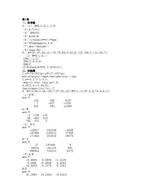
4. A=[3,54,2;34,-45,7;87,90,15];B=[1,-2,67;2,8,74;9,3,0];
(1)A*B
ans =
129
432
4197
7
-407
-1052
end display(sqrt(s*6)) 向量运算
n=input('input n:'); k=1:n; display(sqrt(sum(1./k.^2)*6)) 4. y=0;k=0; while y<3
k=k+1; y=y+1/(2*k-1); end display([k-1,y-1/(2*k-1)]) 5. x0=0;x=1;k=0; a=input('a='); b=input('b='); while abs(x-x0)>=1e-5 && k<500 x0=x; x=a/(b+x0); k=k+1; end display([k,x]); display([(-b+sqrt(b^2+4*a))/2,(-b-sqrt(b^2+4*a))/2]);
1. P=pascal(5);H=hilb(5); Dp=det(P);Dh=det(H);
Kp=cond(P);Kh=cond(H); P 矩阵的性能更好,因为 Kp 较小 2. A=[1,-1,2,3;0,9,3,3;7,-5,0,2;23,6,8,3] B=[3,pi/2,45;32,-76,sqrt(37);5,72,4.5e-4;exp(2),0,97] A1=diag(A);B1=diag(B); A2=triu(A);B2=triu(B); A3=tril(A);B3=tril(B); rA=rank(A);rB=rank(B);
matlab习题2

习题31. 要求在闭区间]2,0[π上产生具有10个等距采样点的一维数组。
试用两种不同的指令实现。
〖提示〗用“:”产生10个等距采样点一维数组;用linspace(a,b,n)产生10个等距采样点一维数组2. 由指令rand('state',0),A=rand(3,5)生成二维数组A ,试求该数组中所有大于0.5的元素的位置,分别求出它们的“全下标”和“单下标”。
〖提示〗rand('state',0)---将随机发生器置为0状态〖答案〗大于0.5的元素的全下标行号 1 3 2 3 3 2 3 1 2 列号 1 1 2 2 3 4 4 5 5大于0.5的元素的单下标1 3 5 6 9 11 12 13 143. 下列命令执行后,L1、L2、L3、L4的值分别是多少? A=1:9;B=10-A; L1=A= =B; L2=A<=5;L3=A>3&A<7;L4=find(A>3&A<7);〖答案〗L1 = 0 0 0 0 1 0 0 0 0L2 = 1 1 1 1 1 0 0 0 0 L3 = 0 0 0 1 1 1 0 0 0 L4 = 4 5 64. 已知矩阵⎥⎦⎤⎢⎣⎡=4321A ,运行指令B1=A.^(2), B2=A^(2), 可以观察到不同运算方法所得结果不同。
(1)请分别写出根据B1, B2恢复原矩阵A 的程序。
(2)用指令检验所得的两个恢复矩阵是否相等。
5. 在时间区间 [0,10]中,绘制tey t2cos 15.0--=曲线。
要求分别采取“标量循环运算法”和“数组运算法”编写两段程序绘图。
〖答案〗51000.511.5ty 151000.511.5ty 26. 先运行clear,format long,rand('state',1),A=rand(3,3),然后根据A 写出两个矩阵:一个对角阵B ,其相应元素由A 的对角元素构成;另一个矩阵C ,其对角元素全为0,而其余元素与对应的A 阵元素相同。
sigma在matlab中的用法

sigma在matlab中的用法
在MATLAB中,sigma(Σ)用于求解求和运算。
语法:
1. 基本形式: sigma(expression, variable, start, end)
2. 完整形式: sigma(expression, variable, start, end, increment)
参数说明:
- expression:表示要求和的表达式。
可以是常数、变量、向量、矩阵、函数等。
- variable:表示求和变量的符号。
- start:表示求和变量的起始值。
- end:表示求和变量的结束值。
- increment(可选):表示求和变量的递增量。
示例:
1. 对向量进行求和:
```
a = [1, 2, 3, 4, 5];
result = sigma(a(i), i, 1, 5);
```
2. 对矩阵的列进行求和:
```
A = [1, 2, 3; 4, 5, 6; 7, 8, 9];
result = sigma(A(:, i), i, 1, 3);
```
3. 对函数进行求和:
```
f = @(x) x^2;
result = sigma(f(x), x, 1, 10);
```
4. 指定递增量的求和运算:
```
result = sigma(a(i), i, 1, 10, 2);
```
以上是sigma在MATLAB中的一些基本用法,根据具体的问题需求,可以灵活运用sigma函数来求解各种求和运算。
Matlab试题库1

一、填空1、在MATLAB命令窗口中的“>>”标志为MATLAB的_______提示符,“│”标志为_______提示符。
2、MATLAB的工作空间中只有三个变量v1, v2, v3,写出把它们保存到文件my_data.mat中的指令_______;3、设x是一维数组,x的倒数第3个元素表示为;设y为二维数组,要删除y的第34行和48列,可使用命令; ;4、fix(-1.5)= , round(-1.5)= .5、x为0~4pi,步长为0.1pi的向量,使用命令_______创建。
6、A=[1,2,3;4,5,6]; A(4)=__________, A(3,2)=__________________7、输入矩阵A=[1 3 2;3 -5 7;5 6 9],使用全下标方式用_______取出元素“-5”,使用单下标方式用_______取出元素“-5”。
8、在Matlab中执行语句C=rem(25,4)的结果为。
9、Matlab的运算符分为算术运算符、关系运算符和。
10、在Matlab中圆周率π用来表示,非数值用来表示。
11、在Matlab中对数值2.3进行向∞方向取整的语句是。
12、在Matlab中命令可以在命令窗口中显示MATLAB函数或者命令的帮助信息。
13、在Matlab中__ 用于括住字符串。
14、Matlab通过数据类型把一组不同类型但同时又是在逻辑上相关的数据组成一个有机的整体,以便于管理和引用。
15、A=[1,2;3,1];B=[1,0;0,1];A~=B= 。
16、是Matlab的主要交互窗口,用于输入命令并显示(除图形以外)的执行结果。
17、在Matlab中引入矩阵除法的概念,有左除右除两种除法,若AX=B,则X= ,若XA=B,则X= 。
18、在Matlab语言中变量的命名应遵循如下规则:变量名必须以开头,大小写,变量名长度不超过位。
19、Matlab中Inf或inf表示、eps表示、NaN表示。
- 1、下载文档前请自行甄别文档内容的完整性,平台不提供额外的编辑、内容补充、找答案等附加服务。
- 2、"仅部分预览"的文档,不可在线预览部分如存在完整性等问题,可反馈申请退款(可完整预览的文档不适用该条件!)。
- 3、如文档侵犯您的权益,请联系客服反馈,我们会尽快为您处理(人工客服工作时间:9:00-18:30)。
arXiv:physics/0612031v1 [physics.atom-ph] 4 Dec 2006
I.
INTRODUCTION
Spectroscopy of heteronuclear diatomic alkali molecules provides important input to current research in cold molecules and mixtures of ultracold atomic gases. Cold heteronuclear alkali dimers are subject to a large interest since they can be formed at temperatures below 1 mK [1, 2, 3, 4, 5] and possess a large permanent electric dipole moment for deeply bound singlet levels [6, 7]. This combination of properties enables electric field control of ultracold collisions [8, 9] and cold chemical reactions [10, 11] and holds promises for applications in quantum computation [12]. Precise potential energy curves, in particular for the lowest electronic states, are evidently important for such applications as well as for understanding the molecule formation processes (photoassociation), ro-vibrational state selective detection [5, 13] and for formation of vibrational ground-state molecules [14]. In ultracold mixtures of atomic gases, quantum degeneracy of one atomic species can be achieved through sympathetic cooling by the other species [15, 16, 17]. The interspecies interaction strength can be varied through magnetic Feshbach resonances and has a large influence on a variety of effects such as phase-separation between a Bose-Einstein condensate and a degenerate Fermi gas [18] and the transition to a Bardeen-Cooper-Schrieffer superfluid state in dilute Fermi gases [19]. Understanding interspecies collision properties at the atomic ground state asymptotes, e.g. predicting the magnetic field strength values of Feshbach resonances at zero kinetic energy, requires precise potential curves of the electronic ground states. Cold LiCs molecules were observed very recently, being formed in a two-species magneto-optical trap [1]. Previ-
The X1 Σ+ and a3 Σ+ states of LiCs studied by Fourier-transform spectrosco Pashov,2 Horst Kn¨ ockel,1 and Eberhard Tiemann1
1
Institut f¨ ur Quantenoptik, Gottfried Wilhelm Leibniz Universit¨ at Hannover, Welfengarten 1, 30167 Hannover, Germany 2 Department of Physics, Sofia University, 5 James Bourchier Boulevard, 1164 Sofia, Bulgaria (Received February 2, 2008) We present the first high-resolution spectroscopic study of LiCs. LiCs is formed in a heat pipe oven and studied via laser-induced fluorescence Fourier-transform spectroscopy. By exciting molecules through the X1 Σ+ -B1 Π and X1 Σ+ -D1 Π transitions vibrational levels of the X1 Σ+ ground state have been observed up to 3 cm−1 below the dissociation limit enabling an accurate construction of the potential. Furthermore, rovibrational levels in the a3 Σ+ triplet ground state have been observed because the excited states obtain sufficient triplet character at the corresponding excited atomic asymptote. With the help of coupled channels calculations accurate singlet and triplet ground state potentials were derived reaching the atomic ground state asymptote and allowing first predictions of cold collision properties of Li + Cs pairs.
∗ Now at Institute of Physics and Astronomy, University of Aarhus, Denmark.
ously, inelastic collisions [20] and sympathetic cooling of Li by Cs in an optical dipole trap [21] have been studied. Recent theoretical work considers LiCs in strong dc electric fields and its influence on rovibrational dynamics [22] and Li-Cs collision cross sections [9]. Although LiCs was observed already in 1928 by Walter and Barratt through absorption in a mixture of metallic vapors [23], very few and no high-resolution spectroscopic studies have been made until now. In the 1980’s Vadla et al. studied the repulsive Li(2p)+Cs(6s) asymptote [24]. More recently LiCs molecules were formed on He nanodroplets and excitation spectra of the d3 Π ← a3 Σ+ transition were recorded and modeled [25]. Ab initio potentials were calculated by Korek et al. [26] (see Fig. 1) and more recently an extended theoretical study was done by Aymar and Dulieu [6]. The theoretical potentials provide a good starting point for analysis of the spectra obtained in the present work. Here we present a high-resolution spectroscopic study of the LiCs molecule. Similar to our previous studies [27, 28] we apply Fourier-transform spectroscopy of laserinduced fluorescence from LiCs molecules formed in a heat-pipe, because this technique is suitable for collecting a large amount of accurate experimental data. By using properly chosen excitation schemes (see e.g. [27, 28]) we can measure transition frequencies to a wide range of vibrational levels in the singlet X1 Σ+ as well as in the triplet a3 Σ+ ground states, especially levels close to the asymptote. Since the two states are coupled at long internuclear distances by the hyperfine interaction it is not correct to treat them separately in this region, as it would lead to model potentials which are unable to reproduce the experimental observations close to the asymptote. Therefore, the aim of our experimental work is to collect experimental data on both ground states and to fit accurate experimental potential energy curves simultaneously for both states - the indispensable starting point for a study of the molecular structure of LiCs or for modeling of cold collision processes on the Li(2s)+Cs(6s) asymptote. We apply these potential curves within a cou-