EVIDENCE OF SHEAR-WAVE ANISOTROPY IN THE UPPER CRUST OF CENTRAL ITALY
横波各向异性在安棚地区裂缝评价中的应用

摘要:横波在各向异性地层中传播会产生分裂现象,裂缝面与井轴平行或斜交的天然裂缝或诱导缝能够造成横波
的各向异性特征,各向异性的大小反映裂缝的发育程度,快横波的偏振方向代表裂缝的走向。可以利用偶极声波成像
测井资料提取的快、慢横波信息,得到地层各向异性的大小,来定性评价安棚地区裂缝的有效性和走向。
关键词:裂缝;声波;横波;走向;各向异性
方向,并进一步确定各向异性的大小。但同时仍需要
结合其它的测井资料,如常规资料和声、电成像资料 等来确定引起各向异性的原因,各向异性的现象在裂 缝性地层中存在,在地应力不平衡的非裂缝性地层中 也同样存在。一般认为,处于应力非平衡状态的非裂 缝性地层中存在与最大水平主应力方向平行的“微裂 缝”。在应用快、慢横波评价地应力方向和裂缝走向 时,应该注意排除岩性和岩石构造变化的影11[句141,下面 是对一些典型的各向异性现象的解释5】。
收稿日期:2007—08—06
修订日期:2007一I 1—25
作者简介:申辉林(1962一),男,吉林安图人,在读博士研究生,地球物理测井,(Tel)13589970006(E—mail)hlshin006@sina.com
万方数据
·374·
新疆石油地质
2008年
图2各向异性地层横波产生分裂示意
由图4b声成像图中可看出,泌x1井3 220—3 224 m地层中裂缝不发育,且井壁有脱落,井眼呈明显的 椭圆状,地层各向异性是由地应力的不均衡引起,快 横波方位角大约在1 100左右,即为现今最大水平主 应力的方向。图4c是该井3 231—3 234m的成像测井 资料,发育两条垂直缝,计算的快横波方位角为110。 左右,裂缝系统的主要走向,与该区域最大水平主应 力方向一致,因此这组裂缝的区域有效性较强。
latex英文模板

\documentclass{article}\usepackage{graphicx}\usepackage[round]{natbib}\bibliographystyle{plainnat}\usepackage[pdfstartview=FitH,%bookmarksnumbered=true,bookmarksopen=true,%colorlinks=true,pdfborder=001,citecolor=blue,%linkcolor=blue,urlcolor=blue]{hyperref}\begin{document}\title{Research plan under the Post-doctorate program at xx University}%\subtitle{aa}\author{Robert He}\date{2008/04/23}\maketitle\section{Research Title}~~~~Crustal seismic anisotropy in the xx using Moho P-to-S converted phases.\section{Research Background \& Purposes}~~~~Shear-wave splitting analyses provide us a new way to study the seismic structure and mantle dynamics in the crust and mantle. The crustal anisotropy is developed due to various reasons including lattice-preferred orientation (LPO) of mineral crystals and oriented cracks.\newlineTraditionally, the earthquakes occurring in the curst and the subducting plates are selected to determine the seismic anisotropy of the crust. However, none of these methods can help us to assess the anisotropy in the whole crust. Because crustal earthquakes mostly are located in the upper crust, they do not provide information of lower crust. On the other hand, earthquakes in the subducting plates provide information of the whole crust but combined with upper mantle. However, it’s difficult to extract the sole contri bution of the crust from the measurement. Fortunately P-to-S converted waves (Ps) at the Moho are ideal for investigation of crustal seismic anisotropy since they are influenced only by the medium above the Moho.Moho. Figure \ref{crustalspliting}~schematically shows the effects of shear wave splitting on Moho Ps phases. Initially, a near-vertically incident P wave generates a radially polarized converted shear wave at the crust-mantle boundary. The phases, polarized into fast and slow directions, progressively split in time as they propagate through the anisotropic media. Here, the Ps waves can be obtained from teleseismic receiver function analysis.%%\begin{figure}[htbp]\begin{center}\includegraphics[width=0.47\textwidth]{crustalsplit.png}\caption{The effects of shear wave splitting in the Moho P to S converted phase. Top shows a schematic seismogram in the fast/slow coordinate system with split horizontal Ps components.(cited from: McNamara and Owens, 1993)}\label{crustalspliting}\end{center}\end{figure}%%The Korean Peninsula is composed of three major Precambrian massifs, the Nangrim, Gyeongii, and Yeongnam massifs(Fig.\ref{geomap}). The Pyeongbuk-Gaema Massif forms the southern part of Liao-Gaema Massif of southern Manchuria, and the Gyeonggi and Mt. Sobaeksan massifs of the peninsula are correlated with the Shandong and Fujian Massifs of China.%\begin{figure}[htbp]\begin{center}\includegraphics[width=0.755\textwidth]{geo.png}\caption{Simplified geologic map. NCB: North China block; SCB: South China block.(cited from: Choi et al., 2006)}\label{geomap}\end{center}\end{figure}%Our purpose of the study is to measure the shear wave splitting parameters in the crust of the Korean Peninsula. The shear wave splitting parameters include the splitting time of shear energybetween the fast and slow directions, as well as fast-axis azimuthal direction in the Korean Peninsula. These two parameters provide us constraints on the mechanism causing the crustal anisotropy. From the splitting time, the layer thickness of anisotropy will be estimated. Whether crustal anisotropy mainly contributed by upper or lower crustal or both will be determined. Based on the fast-axis azimuthal direction, the tectonic relation between northeastern China and the Korean peninsula will be discussed.\section{Research Methods}~~~~Several methods have been introduced for calculation of receiver functions. An iterative deconvolution technique may be useful for this study since it produces more stable receiver function results than others. The foundation of the iterative deconvolution approach is aleast-squares minimization of the difference between the observed horizontal seismogram and a predicted signal generated by the convolution of an iteratively updated spike train with the vertical-component seismogram. First, the vertical component is cross-correlated with the radial component to estimate the lag of the first and largest spike in the receiver function (the optimal time is that of the largest peak in the absolute sense in the cross-correlation signal). Then the convolution of the current estimate of the receiver function with the vertical-component seismogram is subtracted from the radial-component seismogram, and the procedure is repeated to estimate other spike lags and amplitudes. With each additional spike in the receiver function, the misfit between the vertical and receiver-function convolution and the radial component seismogram is reduced, and the iteration halts when the reduction in misfit with additional spikes becomes insignificant.\newlineFor all measurement methods of shear-wave splitting, time window of waveform should be selected. Conventionally the shear-wave analysis window is picked manually. However, manual window selection is laborious and also very subjective; in many cases different windows give very different results.\newlineIn our study, the automated S-wave splitting technique will be used, which improves the quality of shear-wave splitting measurement and removes the subjectivity in window selection. First, the splitting analysis is performed for a range of window lengths. Then a cluster analysis isapplied in order to find the window range in which the measurements are stable. Once clusters of stable results are found, the measurement with the lowest error in the cluster with the lowest variance is presented for the analysis result.\section{Expected results \& their contributions}~~~~First, the teleseismic receiver functions(RFs) of all stations including radial and transverse RFs can be gained. Based on the analysis of RFs, the crustal thickness can be estimated in the Korean Peninsula. Then most of the expected results are the shear-wave splitting parameters from RFs analysis in the crust beneath the Korean Peninsula. The thickness of anisotropic layer will be estimated in the region when the observed anisotropy is assumed from a layer of lower crustal material.All the results will help us to understand the crustal anisotropy source.\newlineCrustal anisotropy can be interpreted as an indicator of the crustal stress/strain regime. In addition, since SKS splitting can offer the anisotropy information contributed by the upper mantle but combined with the crust, the sole anisotropy of the upper mantle can be attracted from the measurement of SKS splitting based on the crustal splitting result.%\cite{frogge2007}%%%\citep{frogge2008}%%%\citep{s-frogge2007}% 5. References\begin{thebibliography}{99}\item Burdick, L. J. and C. A. Langston, 1977, Modeling crustal structure through the use of converted phases in teleseismic body waveforms, \textit{Bull. Seismol. Soc. Am.}, 67:677-691.\item Cho, H-M. et al., 2006, Crustal velocity structure across the southern Korean Peninsula from seismic refraction survey, \textit{Geophy. Res. Lett.} 33, doi:10.1029/2005GL025145.\item Cho, K. H. et al., 2007, Imaging the upper crust of the Korean peninsula by surface-wave tomography, \textit{Bull. Seismol. Soc. Am.}, 97:198-207.\item Choi, S. et al., 2006, Tectonic relation between northeastern China and the Korean peninsula revealed by interpretation of GRACE satellite gravity data, \textit{Gondwana Research}, 9:62-67.\item Chough, S. K. et al., 2000, Tectonic and sedimentary evolution of the Korean peninsula: a review and new view, \textit{Earth-Science Reviews}, 52:175-235.\item Crampin, S., 1981, A review of wave motion in anisotropic and cracked elastic-medium, \textit{Wave Motion}, 3:343-391.\item Fouch, M. J. and S. Rondenay, 2006, Seismic anisotropy beneath stable continental interiors, \textit{Phys. Earth Planet. Int.}, 158:292-320.\item Herquel, G. et al., 1995, Anisotropy and crustal thickness of Northern-Tibet. New constraints for tectonic modeling, \textit{Geophys. Res. Lett.}, 22(14):1 925-1 928.\item Iidaka, T. and F. Niu, 2001, Mantle and crust anisotropy in the eastern China region inferred from waveform splitting of SKS and PpSms, \textit{Earth Planets Space}, 53:159-168.\item Kaneshima, S., 1990, Original of crustal anisotropy: Shear wave splitting studies in Japan, \textit{J. Geophys. Res.}, 95:11 121-11 133.\item Kim, K. et al., 2007, Crustal structure of the Southern Korean Peninsula from seismic wave generated by large explosions in 2002 and 2004, \textit{Pure appl. Geophys.}, 164:97-113.\item Kosarev, G. L. et al., 1984, Anisotropy of the mantle inferred from observations of P to S converted waves, \textit{Geophys. J. Roy. Astron. Soc.}, 76:209-220.\item Levin, V. and J. Park, 1997, Crustal anisotropy in the Ural Mountains foredeep from teleseismic receiver functions, \textit{Geophys. Res. Lett.}, 24(11):1 283 1286.\item Ligorria, J. P. and C. J. Ammon, 1995, Iterative deconvolution and receiver-function estimation. \textit{Bull. Seismol. Soc. Am.}, 89:1 395-1 400.\item Mcnamara, D. E. and T. J. Owens, 1993, Azimuthal shear wave velocity anisotropy in the basin and range province using Moho Ps converted phases, \textit{J. Geophys. Res.}, 98:12003-12 017.\item Peng, X. and E. D. Humphreys, 1997, Moho dip and crustal anisotropy in northwestern Nevada from teleseismic receiver functions, \textit{Bull. Seismol. Soc. Am.}, 87(3):745-754.\item Sadidkhouy, A. et al., 2006, Crustal seismic anisotropy in the south-central Alborz region using Moho Ps converted phases, \textit{J. Earth \& Space Physics}, 32(3):23-32.\item Silver, P. G. and W. W. Chan, 1991, Shear wave splitting and subcontinental mantle deformation, \textit{J. Geophys. Res.},96:16 429-16454.\item Teanby, N. A. et al., 2004, Automation of shear wave splitting measurement using cluster analysis, \textit{Bull. Seismol. Soc. Am.}, 94:453-463.\item Vinnik, L. and J-P. Montagner, 1996, Shear wave splitting in the mantle Ps phases,\textit{Geophys. Res. Lett.}, 23(18):2 449- 2 452.\item Yoo, H. J. et al., 2007, Imaging the three-dimensional crust of the Korean peninsula by joint inversion of surface-wave dispersion of teleseismic receiver functions, \textit{Bull. Seismol. Soc. Am.}, 97(3):1 002-1 011.\item Zhu, L., and H. Kanamori, 2000, Moho depth variation in Southern California from teleseismic receiver functions, \textit{J. Geophys. Res.}, doi :10.1029/1999JB900322, 105:2 969-2 980.%%%%\end{document}。
六种不同变质程度煤的纵横波速度特征及其与密度的关系

六种不同变质程度煤的纵横波速度特征及其与密度的关系王赟;许小凯;张玉贵【摘要】A lab ultrasonic measurement of six metamorphic kinds of coals was conducted under 25℃ and 0. 1 MPa condition. And then some phenomena were concluded as follows: There are better linear correlations between pressure wave (P-wave) velocity and density, shear wave (S-wave) velocity and density; and the correlation coefficients of strike, dip and vertical directions are different and decreasing. Also there are positive linear correlation between P- and S-wave velocity in the same direction. However, there are great difference between velocities of different directions, especially in the strike and the vertical direction. The average anisotropy is about 0. 1 and even more. Through comparing and analyzing the measured values with the estimated values, according to Gardner and Castagna formula, a non-tolerated error was found, which means that these two experience formulas cannot be applied to coal, and a suitable coal formula should bernused in coal seam seismic exploration.%对采自不同地区和煤矿的六种不同变质程度煤样进行常温常压条件下的超声测量.测量发现:煤的纵波与横波速度均与密度存在良好的线性正相关关系,且沿煤层走向、倾向和垂直煤层层理方向的纵横波速度逐渐降低;走向、倾向和垂向上的纵波速度与同一方向的横波速度也存在良好的线性正相关性;六种煤样三个方向间的速度各向异性一般都大于10%.通过与经典经验公式—Gardner与Castagna公式理论换算值的对比发现:由于煤层的软岩特征,理论换算煤的纵波速度、横波速度与实验室实测值之间存在较大误差.因此,在煤田地震勘探中应使用根据煤的岩石物理测试而形成的关系式.【期刊名称】《地球物理学报》【年(卷),期】2012(055)011【总页数】8页(P3754-3761)【关键词】纵波;横波;速度;密度;各向异性【作者】王赟;许小凯;张玉贵【作者单位】中国科学院地球化学研究所,贵阳 550002;河南理工大学瓦斯地质研究所,焦作 454003;河南理工大学瓦斯地质研究所,焦作 454003【正文语种】中文【中图分类】P6311 引言随着煤炭资源开采深度的加大,深部高温热害和深层煤与瓦斯突出等动力学灾害的危险程度逐渐增加,对煤田地震勘探精度的要求也逐渐提高.目前,煤田勘探不仅要求地震勘探预测小断层,还要求对深层煤层顶底板岩性、构造煤分布、瓦斯富集程度等情况进行定性或定量的预测.随着煤层气资源勘探开发力度的加大,水平井技术得以广泛的应用,煤层气开发方案的确定,需要提前精确预测煤层厚度和煤层裂缝的发育程度与发育方向.因此,煤田地震与测井约束反演方法逐渐在煤田勘探中得到应用与推广[1].正如油气田地震反演技术应用一样,煤田地震的反演也需要煤的密度、速度及其相互换算的定量关系支持,以降低地震反演中的不确定性与多解性.由于煤层是典型的软岩,因此取芯和制样难度较大.而且由于以前煤田地震勘探主要以构造勘探为主,对于煤的声学弹性模量并无要求,使得国内外对于煤的声学特征的研究相对较少.在煤的弹性参数测量的两种方法中,以静态法研究较多[2-7],主要是利用三轴应力—应变测试技术进行煤岩变形测量与弹性模量计算,目的是通过煤岩的力学参数的测量服务于井下巷道开采工程.由于动态法可以方便地模拟地层条件,从而使得动态法测量的弹性参数对实际地球物理勘探的指导意义更为明显,朱国维等[8]通过改变温度与压力来模拟地层条件,测试了淮南某矿区13-1煤的声波速度与煤层埋深的关系;孟召平等[9]在大量测井与钻孔数据统计分析的基础上,研究煤岩纵、横波速度与砂岩和灰岩的纵、横波速度的差异;郭德勇等[10]对原生结构煤在高压条件下不同方位波速变化进行了测试,研究了煤的纵波速度的各向异性特征;赵群、郝守玲[11]和董守华[12]在此基础上进一步测量研究了煤岩衰减系数、横波速度等的各向异性特征;汤红伟、程建远[13]等人对采自深层的煤样进行了超声测量,主要研究温度、压力和含水饱和度的变化对纵波与横波速度的影响.由于煤层制样难,李建楼[14]、张平松[15]等采用井下巷道现场声波探测方法对煤体的速度特征进行了研究.由于煤炭并非国外的主要能源,加之国外的煤田构造简单,国际上对煤岩的弹性测量研究较少.Yao和Han[16]从烃源岩的角度对煤及其相似的页岩和碳质泥岩进行了实验室的超声测量,讨论了压力、温度与含水饱和度对煤岩样速度和各向异性的影响;并通过与测井数据的对比和合成地震记录重点说明煤系地层的地震反射特征及其对油气储层反射特征的影响.对于国内煤田勘探而言,随着阻抗反演的推广应用,对于煤弹性模量特征的研究需求越来越多.但目前已有的煤弹性参数的测量结果都比较零散,只涉及一种变质程度煤或某几个煤矿的具体矿区的试验,对于不同变质程度煤的弹性特征缺少系统性的认识.因此本文针对采自国内不同地区的、不同变质程度煤的弹性速度进行了实验室测量,探索煤速度-密度、纵波速度-横波速度之间的关系,并通过与经典Gardner公式[17]、Lindseth公式[18]和Castagna公式[19]的对比,尝试总结具有普遍适用性的煤速度-密度、纵波速度-横波速度的经验公式,以方便煤田地震勘探的应用;并着重说明煤弹性参数的特殊性及其应用于煤田地震反演需要注意的问题.2 原煤样品弹性测试2.1 待测样品信息为了探索我国主要变质类型煤的弹性参数特征,我们采集了国内不同地区、不同煤矿、具有不同变质程度的六种原生结构煤.为了使实验室测量的煤弹性性质能给煤田地震与测井的联合反演提供直接的物理参数,我们在井下采取煤层定向煤样,即煤样采集时标注煤层的层理方向和走向、倾向,在实验室中经过磨制加工成6cm×6cm×6cm的立方体,共25块;选择其中相对完整的8块进行常温(25℃)、常压(1个大气压)条件下的超声测量和密度测量;样品信息见表1、图1所示.实验中只研究垂直层理方向、倾向、走向三个主要方向,而不涉及平行层理方向平面内的方位声学各向异性.本文所指的密度为视密度,又称视相对密度,即地勘行业所使用的密度.密度测量按照国家行业规范[20]由河南理工大学测量.图1 待测煤样Fig.1 Photos of testing samples表1 测试样品信息Table 1 Coal samples under testing样品编号采样地点煤样变质程度加工规格A义马煤矿褐煤 6cm 见方B 平顶山八矿戊组肥煤 6cm见方C1 平顶山八矿己组焦煤 6cm见方C2 平顶山八矿己组焦煤 6cm见方D新疆气煤 6cm见方E 鹤壁六矿2143工作面贫瘦煤 6cm见方F1 焦作方庄矿无烟煤6cm见方F2 焦作九里山矿无烟煤 6cm见方1)伍向阳.石油流体中声波速度及其相关性质研究.北京:中国科学院地球物理研究所,2000,3.1.2.2 超声测量本次超声试验采用常温常压行波传播—脉冲透射的方法进行测试1).整套仪器由脉冲信号发生器、超声换能器、放大器、计数器和示波器组成,如图2所示.实验使用的是压电陶瓷柱状纵横波换能器.为保证样品与换能器耦合良好,测试纵波时采用凡士林进行耦合;测试横波时采用蜂蜜耦合.由于测试煤样为边长6cm的立方体,选用超声的低频段,纵波主频为100kHz,横波主频为250kHz,整个测量系统误差小于1%;考虑到煤岩的特殊性,最大误差不超过3%.图2 数字化脉冲法声波测试系统框图Fig.2 Diagram of digital pulse sonic testing system本次超声测量选取相对较完整、具有平整平面的样品,分别测量了煤样沿煤层走向、倾向和垂向(垂直层理)3个方向的纵横波速度;同时还测量了一个与煤样尺寸相同的标准铝块,如图3所示.为与煤田人工地震的观测方式相统一,分别以x、y、z代表煤层的走向、倾向和垂直层理的方向.如图3所示,Vx、Vy、Vz分别表示沿煤层走向、倾向和垂直层理的纵波速度.横波振动方向与波前方向垂直,由于煤样中裂隙的存在,横波通过煤样传播会分裂成两个相互垂直的横波,所以横波沿煤样某个方向传播时会有两个速度值.以沿x方向传播为例,沿x方向传播的横波有Vxy与Vxz,下标的第一个字母x代表横波传播的方向,第二个字母代表与传播方向垂直的方向(即横波振动方向).即Vxy表示横波沿x传播,振动方向与y平行;Vxz表示沿x传播,振动方向与z平行.纵横波速度计算采用1)图3 煤样测速示意图Fig.3 Schematic diagram of ultra-sonic measurement ofcoal sample其中:Vp为纵波速度,单位m·s-1;Vs为横波速度,单位m·s-1;L为发射、接收换能器中心间的距离,单位m;tp为纵波在样品中的走时,单位s;ts为横波在样品中的走时,单位s;t0为仪器系统的零延时,单位s.2.3 测量结果与弹性参数换算原煤样品纵横波测试计算结果见表2、表3.表3中E和F1样品由于裂缝的复杂性导致横波初至难以识别而无法计算横波速度,在本试验中空缺z方向的两个速度. 表2 原煤样品纵波速度测试结果Table 2 P-wave velocity of coals tested in lab 煤样编号样品纵波速度Vp(m·s-1)Vx Vy Vz视密度ARD(g·cm-3)A 2108 1937 1704 1.15 B 2383 1935 1781 1.28 C2 2153 1989 1959 1.35 C1 2235 1889 1629 1.38 D 2183 1986 1770 1.24 E 1959 1634 1479 1.4 F1 2522 2437 2190 1.51 F2 3047 2969 2757 1.73表3 原煤样品横波速度测试结果Table 3 S-wave velocity of coals tested in lab 煤样编号横波速度Vs(m·s-1)Vxy VxzVx均值Vyx VyzVy均值Vzx VzyVz 均值A 1097 1081 1089 971 959 965 910 870 890 B 1079 1046 1063 1018 938 978 800 780 790 C2 1127 977 1052 1108 1080 1094 969 950 960 C1 1264 1139 1202 1066 1012 1039 1001 986 994 D 1060 980 1020 1088 1038 1063 1024 974 999 E 991 977 984 704 694 699 F1 1266 1249 1258 1210 1113 1162 F2 1612 1605 1609 1516 1492 1504 1352 1308 13303 测试数据分析为分析不同变质程度煤的速度与密度的关系,我们在实验中还专项测试了每个煤样的最大镜质组反射率等煤质参数.但由于文章篇幅和论述重点的要求,关于煤的镜质组最大反射率与煤的声波速度之间的关系,我们将在另一篇文章中讨论.以下内容将重点讨论不同变质程度煤的纵波速度-密度、横波速度-纵波速度之间的关系及其特征.3.1 原煤样品纵横波速度与密度关系在地震数据处理、解释和反演中,速度-密度的关系,尤其纵波速度-密度关系是经常要用到的公式.为此,我们针对煤样分析它的纵横波速度与密度的关系,以认识煤的特殊性.如图4和图5所示为三方向纵波速度、横波速度与密度之间的试验散点图和线性回归方程.由图4、图5可以看出各个方向上的纵波速度与横波速度都随着密度增大而增大;即纵波速度、横波速度与密度均存在正线性相关性,平均相关系数0.8.但三方向纵波速度-密度相关性与横波速度-密度相关性规律不同:纵波速度与密度的相关性按走向、垂向、倾向三方向划分依次降低,且3方向相关性差异不大,均在80%附近;而横波速度-密度的相关性按垂向、走向、倾向依次降低,且倾向方向的横波速度-密度的相关性比其它2个方向要差得较大.而且从图4和图5还可以看出,三方向纵波速度与横波速度存在以下的统一性规律:走向速度大于倾向速度,垂向速度最小;走向速度与垂向速度差异较大,倾向速度接近平均速度.3.2 原煤样品纵横波速度间的关系此外,在多波地震的联合反演中,由于横波测井数据较少,一般需要利用纵波速度换算横波速度;而在目前的油气地震反演应用中,一般采用Castagna公式进行弹性阻抗的反演.但对于煤田地震该公式是否合适尚缺乏有效的实验证据.为分析煤纵横波速度间的关系,下面以相同方向的纵波速度Vp为变量,横波速度Vs为因变量做回归分析,见图6.从回归图可以看出Vp与Vs间存在着线性关系,随着纵波速度的增大,横波速度也不断增大,且平均线性相关性大于0.9;其中以倾向和走向方向的纵波速度—横波速度线性相关性最好,大于93%,而垂向的稍差,相关系数为86%.从三方向纵波速度-横波速度回归公式可以看到:三条直线方程基本可以用平均速度的回归公式代替,说明三方向的纵波速度-横波速度关系总体上一致.3.3 三方向纵横波速度的各向异性为了说明煤层三方向速度的差异性,定义两个方向间的速度各向异性以表示[22],如表4所示为速度各向异性的计算结果.从表中数据统计可以得出以下规律:走向与垂向之间的速度差异最大,纵波速度各向异性为9.4%-31.4%,平均20.5%;横波为2.1%-29.5%,平均16.5%.走向与倾向、倾向与垂向之间的速度各向异性基本都在10%左右.表4 纵横波速度的各向异性Table 4 Anisotropy of P-and S-wave velocity注:表中某一方向横波速度是采用了这一方向快慢波速度的平均值.煤样编号纵波速度各向异性(%)横波速度各向异性(%)PAxy PAxz PAyz SAxy SAxz SAy z A 8.5 21.2 12.8 12.1 20.1 8.1 B 20.8 28.9 8.3 8.3 29.5 21.3 C2 7.9 9.4 1.5 3.9 9.1 13 C1 16.8 31.4 14.7 14.5 18.9 9.2 D 9.5 20.9 11.5 4.1 2.1 6.2 E 18.1 27.9 10 33.9 F1 3.4 14.1 10.7 7.9 F2 2.6 10 7.4 8.7 19 12.3均值11 20.5 9.6 11.7 16.5 11.73.4 与经典经验关系式的对比3.4.1 纵波速度-密度换算经验公式在煤田地震数据处理及与测井数据的联合反演中,经常需要用到密度-速度的关系式,以减少反演参数的数量.此外,由于很多煤田测井缺少声波曲线,还经常需要根据密度曲线进行纵波速度的换算.但到目前为止,按照油气领域井震联合反演的方法和商业软件,工程技术人员还习惯于使用Gardner公式[17]进行两者的换算. Gardner公式在油气勘探领域的应用得到了广泛的认可,但对于煤会产生巨大的误差,为此,Lindseth[18]提出了一个改进的经验公式,在沉积岩地区应用效果较为理想.为了对比说明煤纵波速度与密度关系的特殊性,在本次实验的基础上,分别应用Gardner公式、Lindseth公式和本文回归的公式(图4中的垂向回归公式)进行了煤的纵波速度的计算.以实验室测量垂向纵波速度为基准,对比了各公式的相对误差,如表5所示.为与煤田地震勘探相匹配,表中数据计算只考虑了垂直层理方向的纵波速度.表5 纵波速度实验室测量值与经验公式换算值对比Table 5 Comparison between P-wave velocities tested in lab and estimated with empirical formulas煤样编号垂向纵波速度(Vp/(m·s-1))视密度(ARD/(g·cm-3))Gardner公式(Vp/(m·s-1))相对误差(%)Lindseth公式(Vp/(m·s-1))相对误差(%)本文公式(Vp/(m·s-1))相对误差(%)A 1704 1.15 189 89 1632 4 1494 12 B 1781 1.28 291 84 1739 2 1728 3 C2 1959 1.35 360 82 1804 8 1854 5 C1 1629 1.38 393 76 1834 13 1909 17 D 1770 1.24 256 86 1705 4 1656 6 E 1479 1.4 416 72 1853 25 1945 32 F1 2190 1.51 563 74 1970 10 2143 2 F2 2757 1.73 970 65 2256 18 2540 8未知量已知量平均误差78.5 平均误差 10.5 平均误差10.6从表中误差对比可以看到,Lindseth公式和本文回归公式的精度远高于Gardner公式,平均误差10%,基本可以满足地震勘探的精度需要.因此,在缺失声波测井数据,利用密度曲线换算声波速度进行煤田地震与测井的联合反演时,针对我国煤田的纵波速度(垂向)与密度关系,建议采用本文回归的公式:式中Vp为纵波速度,单位m·s-1;ρ为密度,单位g·cm-3,相关系数为81%. 3.4.2 纵波速度—横波速度换算经验公式在弹性阻抗反演过程中,由于横波偶极子测井或三分量VSP测井的缺失,还经常用到Castagna公式[19,22]进行横波速度的求取[23-25].但该公式是否适用于煤有待于检验.为此,在本次实验的基础上,应用Castagna公式和本文回归的公式(图6中的垂向回归公式)进行了煤横波速度的计算.以实验室测量横波速度为基准,对比了各公式的相对误差,如表6所示.为与煤田地震勘探相匹配,表中数据计算只考虑了垂直层理方向的横波速度,实验室测量横波速度取快、慢波的均值. 通过表6中数据对比可以发现,简单套用Castagna公式会产生巨大的误差,而本文所提出的公式平均误差可以控制在10%以内.因此,建议在煤的弹性阻抗反演中,在缺失横波速度的情况下,采用本文回归的平均速度公式约束横波速度的计算,效果会好于采用Castagna公式,相关系数可达0.96.式中Vp为纵波速度,Vs为横波速度,单位m·s-1.因此,对于不同地区、不同变质程度煤的井震联合反演,应根据实际岩心的弹性测量结果使用煤自身的密度—速度、纵波速度—横波速度的回归公式;在缺失实验室测量结果的情况下,应用煤田测井数据回归的公式或本文给出的公式可相对减小反演误差.表6 实测横波速度与经验公式求取值对比Table 6 Comparison between S-wave velocities measured in lab and estimated with empirical formula煤样编号实测垂向横波速度均值(Vs/(m·s-1))Castagna公式求取的垂向横波速度(Vs/(m·s-1))Castagna公式相对误差本文回归公式计算的垂向横波速度(Vs/(m·s-1))本文公式相对误差A 890 297 67 912 2 B 790 363 54 941 19 C2 960 516 46 1008 5 C1 994 241 76 883 11 D 999 353 65 937 6 E 103 826 F1 715 1096 F2 1330 1204 9 1312 1均值994 474 53 999 74 结论与认识通过六种不同变质程度煤层走向、倾向、垂直层理方向(垂向)的超声测量结果分析,可以获得如下的结论:(1)不同变质程度煤的纵波速度、横波速度均与密度存在较好的相关性,平均线性正相关的系数在80%以上.其中走向与垂直层理方向的纵波速度-密度、横波速度-密度的相关性好于倾向方向的速度-密度相关性,这与沉积的物源方向是相吻合的;除倾向方向的速度-密度关系外,横波速度-密度的相关性要好于纵波速度-密度的相关性,这与横波沿骨架传播,不受流体影响也是吻合的.(2)三方向的纵波速度、横波速度与密度的关系均表现为相同的变化规律,即走向方向速度最大,垂向速度最小,倾向方向速度接近于三方向速度的均值.(3)相同方向的纵波速度与横波速度存在良好的线性正相关性,其中走向与倾向的相关性好于垂向;三方向的平均纵波速度与平均横波速度的线性相关性高达96%.(4)煤层三方向纵波速度与横波速度均存在差异,总体表现为纵波的速度各向异性大于横波的速度各向异性;其中以走向与垂向速度之间的差异最大,纵波平均各向异性可达20%;横波平均可达15%;另外两个方向速度的各向异性在10%左右. (5)通过与地震勘探领域的经典纵波速度-密度经验公式和纵波速度-横波速度公式对比发现,Gardner公式描述煤纵波速度-密度的关系存在巨大误差;对中国不同变质程度煤,在缺少足够钻孔和测井数据的情况下,建议使用本文回归公式或Lindseth公式,可将误差控制在10%左右;Castagna公式也不适合于描述煤的纵波速度-横波速度关系,建议使用本文回归的公式,可将误差控制在10%以内.这些在井震联合反演中需要特别注意.随着井震联合反演应用于煤田勘探的精度要求越来越高,对煤纵波速度-密度、纵波速度-横波速度的规律性认识是十分重要的.尽管本文超声测试的煤样偏少,但在不同地区、不同变质程度煤的速度-密度等一般性规律认识缺少,甚至套用油气领域公式存在巨大误差的前提下,本文提出的公式对于煤的精细勘探具有较好参照价值.致谢感谢中国科学院地质与地球物理研究所的伍向阳研究员和中国石油大学(北京)的魏建新研究员在煤的超声测量中给予的指导和帮助.参考文献(References)[1]石瑛,王赟,芦俊.煤田地震多属性分析技术的应用.煤炭学报,2008,33(12):1397-1402.Shi Y,Wang Y,Lu J.Application of seismic multi-attribute analysis technique in coal field.Journal of China Coal Society (in Chinese),2008,33(12):1397-1402.[2]孟召平,彭苏萍,凌标灿.不同侧压下沉积岩石变形与强度特征.煤炭学报,2000,25(1):15-18.Meng Z P,Peng S P,Ling B C.Characters of the deformation and strength under different confining pressures on sedimentary rock.Journal of China Coal Society(in Chinese),2000,25(1):15-18.[3]孟召平,彭苏萍,傅继彤.含煤岩系岩石力学性质控制因素探讨.岩石力学与工程学,2002,21(1):102-106.Meng Z P,Peng S P,Fu J T.Study on control factors of rock mechanics properties of coal-bearing formation.Chinese Journal of Rock Mechanics and Engineering (in Chinese),2002,21(1):102-106.[4]闫立宏.杨庄煤矿煤岩波速特征及与其强度的关系研究.煤炭科学技术,2006,4(6):57-60.Yan L H.Relationship study between characteristics and strength of coal and rock wave velocity in Yangzhuang Mine.Coal Science and Technology (in Chinese),2006,4(6):57-60.[5]彭担任,王占国,周新青等.煤层岩体中声波速度与导热系数的关系.矿业安全与环保,1999,(1):11-14.Peng D R,Wang Z G,Zhou X Q,etal.Relationship between sonic wave velocity and Hest-conductivity coefficient in coal and rock.Mining Safety &Environmental Protection(in Chinese),1999,(1):11-14.[6]孟召平,张吉昌,Tiedemann J.煤系岩石物理力学参数与声波速度之间的关系.地球物理学报,2006,49(5):1505-1510.Meng Z P,Zhang J C,Tiedemann J.Relationship between physical and mechanical parameters and acoustic wave velocity of coal measures rocks.Chinese Journal of Geophysics(in Chinese),2006,49(5):1505-1510.[7]吴基文,姜振泉,樊成等.煤层抗拉强度的波速测定研究.岩土工程学报,2005,27(9):999-1003.Wu J W,Jiang Z Q,Fan C,et al.Study on tensile strength of coal seam by wave velocity.Chinese Journal of Geotechnical Engineering (in Chinese),2005,27(9):999-1003.[8]朱国维,王怀秀,韩堂惠等.地层条件下煤层顶、底板声波速度与反射特征.煤炭学报,2008,33(12):1391-1396.Zhu G W,Wang H X,Han T H,etal.Reflection characteristics and acoustic velocity of coal roof and floor under formation conditions.Journal of China Coal Society(in Chinese),2008,33(12):1391-1396.[9]孟召平,刘常青,贺小黑等.煤系岩石声波速度及其影响因素实验分析.采矿与安全工程学报,2008,25(4):389-393.Meng Z P,Liu C Q,He X H,etal.Experimental research on Acoustic wave velocity of coal measures rocks and its influencing factors.Journal of Mining &Safety Engineering(in Chinese),2008,25(4):390-394.[10]郭德勇,韩德馨,冯志亮.围压下构造煤的波速特征实验研究.煤炭科学技术,1998,26(4):21-24.Guo D Y,Han D X,Feng Z L.Experimental researchon acoustic wave velocity of tectonic coal under confined pressure.Coal Science and Technology (in Chinese),1998,26(4):21-24.[11]赵群,郝守玲.煤样的超声速度和衰减各向异性测试实例.石油地球物理勘探,2005,40(6):708-712.Zhao Q,Hao S L.Testing anisotropy of ultrasonic velocity and attenuation in coal samples.Oil Geophysical Prospecting(in Chinese),2005,40(6):708-712.[12]董守华.气煤弹性各向异性系数实验测试.地球物理学报,2008,51(3):947-952.Dong S H.Test on elastic anisotropic coefficients of gascoal.Chinese Journal of Geophysics(in Chinese),2008,51(3):947-952.[13]汤红伟,程建远,王世东.深层煤矿床的煤岩样物性测试结果与分析.中国煤炭,2009,35(9):75-79.Tang H W,Cheng J Y,Wang S D.The test results and its analysis of deep coal seam and rock sample.China Coal(in Chinese),2009,35(9):75-79.[14]李建楼,严家平.频谱分析技术在煤体结构探测中的应用.煤炭科学技术,2009,37(8):120-123.Li J L,Yan J P.Application of spectrum analysis technology to coal structure exploration.Coal Science and Technology(in Chinese),2009,37(8):120-123.[15]张平松,刘盛东.煤岩体结构构造特征的频谱分析与应用.工程地球物理学报,2006,3(4):274-277.Zhang P S,Liu S D.The structure character of coal and rock by seismic wave spectrum analyzing technology and its application.Chinese Journal of Engineering Geophysics(in Chinese),2006,3(4):274-277.[16]Yao Q L,Han D H.Acoustic properties of coal from labmeasurement.SEG Las Vegas 2008Annual Meeting,1815-1819.[17]Gardner G L F,Gardner L W,Gregory A R.Formation velocity and density-the diagnostic basics for stratigraphic traps.Geophysics,1974,39(6):770-780.[18]Lindseth R O.Synthetic Sonic Logs—aprocess for stratigraphic interpretation.Geophysics,1979,44(1):3-26.[19]Castagna J P,Smith S parison of AVO indicators:A modeling study.Geophysics,1994,59(12):1849-1855.[20]GB/T6949-1998,《煤的视相对密度测定方法》.国家质量技术监督局,1998,1-4.GB/T6949-1998,Determination of apparent relative density of coal (in Chinese).General Administration of Quality Supervision of the People′s Republic of China,1998,1-4.[21]刘斌,席道瑛,葛宁洁等.不同围压下岩石中泊松比的各向异性.地球物理学报,2002,45(6):880-890.Liu B,Xi D Y,Ge N J,et al.Anisotropy of Poisson′s ratio in rock samples under confining pressures.Chinese Journalof Geophysics(in Chinese),2002,45(6):880-890.[22]Greenberg M L,Castagna J P.Shear-wave velocity estimation in porous rocks:theoretical formulation,preliminary verification and applications.Geophysical Prospecting,1992,40(2):195-210.[23]张关泉,屠浩敏.层状弹性介质的波阻抗反演.地球物理学报,1995,38(S):81-93.Zhang G Q,Tu H M.Impedance inversion for elastic layered media.Chinese Journal of Geophysics (in Chinese),1995,38(S):81-93.[24]马劲风.地震勘探中广义弹性阻抗的正反演.地球物理学报,2003,46(1):118-124.Ma J F.Forward modeling and inversion method of generalized elastic impedance in seismic exploration.Chinese Journal of Geophysics(in Chinese),2003,46(1):118-124.[25]彭真明,李亚林,巫盛洪等.碳酸盐岩储层多角度弹性阻抗流体识别方法.地球物理学报,2008,51(3):881-885.Peng Z M,Li Y L,Wu S H,etal.Discriminating gas and water using multi-angle extended elastic impedance inversion in carbonate reservoirs.Chinese Journal of Geophysics (in Chinese),2008,51(3):881-885.。
Surface wave higher-mode phase velocity measurements using a roller- coaster-type algorithm
Geophys.J.Int.(2003)155,289–307Surface wave higher-mode phase velocity measurements usinga roller-coaster-type algorithm´Eric Beucler,∗´El´e onore Stutzmann and Jean-Paul MontagnerLaboratoire de sismologie globale,IPGP,4place Jussieu,75252Paris Cedex05,France.E-mail:beucler@ipgp.jussieu.frAccepted2003May20.Received2003January6;in original form2002March14S U M M A R YIn order to solve a highly non-linear problem by introducing the smallest a priori information,we present a new inverse technique called the‘roller coaster’technique and apply it to measuresurface wave mode-branch phase velocities.The fundamental mode and thefirst six overtoneparameter vectors,defined over their own significant frequency ranges,are smoothed averagephase velocity perturbations along the great circle epicentre–station path.These measurementsexplain well both Rayleigh and Love waveforms,within a maximum period range includedbetween40and500s.The main idea of this technique is tofirst determine all possibleconfigurations of the parameter vector,imposing large-scale correlations over the model space,and secondly to explore each of them locally in order to match the short-wavelength variations.Thefinal solution which achieves the minimum misfit of all local optimizations,in the least-squares sense,is then hardly influenced by the reference model.Each mode-branch a posteriorireliability estimate turns out to be a very powerful instrument in assessing the phase velocitymeasurements.Our Rayleigh results for the Vanuatu–California path seem to agree correctlywith previous ones.Key words:inverse problem,seismic tomography,surface waves,waveform analysis.1I N T R O D U C T I O NOver the last two decades,the resolution of global tomographic models has been greatly improved,because of the increase in the amount and the quality of data,and due to more and more sophisticated data processing and inversion schemes(Woodhouse&Dziewonski1984, 1986;Montagner1986;Nataf et al.1986;Giardini et al.1987;Montagner&Tanimoto1990;Tanimoto1990;Zhang&Tanimoto1991; Su et al.1994;Li&Romanowicz1995;Romanowicz1995;Trampert&Woodhouse1995;Laske&Masters1996;Ekstr¨o m et al.1997; Grand et al.1997;van der Hilst et al.1997;Liu&Dziewonski1998;Ekstr¨o m&Dziewonski1998;Laske&Masters1998;M´e gnin& Romanowicz2000;Ritsema&van Heijst2000,among others).These models are derived from surface wave phase velocities and/or body wave traveltimes(or waveforms)and/or free-oscillation splitting measurements.Body wave studies provide high-resolution models but suffer from the inhomogeneous distribution of earthquakes and recording stations,even when considering reflected or diffracted phases.On the other hand,the surface wave fundamental mode is mainly sensitive to the physical properties of the upper mantle.So,the investigation of the transition zone on a global scale,which plays a key role in mantle convection,can only be achieved by using higher-mode surface waves.Afirst attempt at providing a global tomographic model using these waves has been proposed by Stutzmann&Montagner(1994),but with a limited amount of data.More recently,van Heijst&Woodhouse(1999)computed degree-12phase velocity maps of the fundamental mode and the fourfirst overtones for both Love and Rayleigh waves.These data have been combined with body wave traveltimes measurements and free-oscillation splitting measurements,to provide a global tomographic model with a high and uniform resolution over the whole mantle (Ritsema et al.1999;van Heijst et al.1999).The most recent S H model for the whole mantle was proposed by M´e gnin&Romanowicz (2000).This degree-24model results from waveform inversion of body and surface Love waves,including fundamental and higher modes and introducing cross-branch coupling.Extracting information from higher-mode surface waves is a difficult task.The simultaneous arrivals(Fig.3in Section3)and the interference between the different mode-branches make the problem very underdetermined and non-linear.To remove the non-linearity,Cara &L´e vˆe que(1987)and L´e vˆe que et al.(1991)compute the cross-correlogram between the data and monomode synthetic seismograms and ∗Now at:´Ecole Normale Sup´e rieure,24rue Lhomond,75231Paris Cedex05,France.C 2003RAS289290´E.Beucler,´E.Stutzmann and J.-P.Montagnerinvert the amplitude and the phase of thefiltered cross-correlogram.On the other hand,Nolet et al.(1986)and Nolet(1990)use an iterative inverse algorithm tofit the waveform in the time domain and increase the model complexity within the iterations.These two methods provide directly a1-D model corresponding to an average epicentre–station path.They werefirst used‘manually’,which limited the amount of data that could be processed.The exponential increase in the amount of good-quality broad-band data has made necessary the automation of most parts of the data processing and an automatic version of these methods has been proposed by Debayle(1999)for the waveform inversion technique of Cara&L´e vˆe que(1987)and by Lebedev(2000)and Lebedev&Nolet(2003)for the partition waveform inversion.Stutzmann&Montagner(1993)split the inversion into two steps;at each iteration,a least-squares optimization to measure phase velocities is followed by an inversion to determine the1-D S-wave velocity model,in order to gain insight into the factors that control the depth resolution.They retrieve the phase velocity for a set of several seismograms recorded at a single station and originating from earthquakes located in the same area in order to improve the resolution.Another approach has been followed by van Heijst&Woodhouse(1997)who proposed a mode-branch stripping technique based on monomode cross-correlation functions.Phase velocity and amplitude perturbations are determined for the most energetic mode-branch,the waveform of which is then subtracted from the seismogram in order to determine the second most energetic mode-branch phase velocity and amplitude perturbations,and so on.More recently,Y oshizawa&Kennett(2002)used the neighbourhood algorithm(Sambridge1999a,b)to explore the model space in detail and to obtain directly a1-D velocity model which achieves the minimum misfit.It is difficult to compare the efficiency of these methods because they all follow different approaches to taking account of the non-linearity of the problem.Up to now,it has only been possible to compare tomographic results obtained using these different techniques.In this paper,we introduce a new semi-automatic inverse procedure,the‘roller coaster’technique(owing to the shape of the misfit curve displayed in Fig.6b in Section3.4.1),to measure fundamental and overtone phase velocities both for Rayleigh and Love waves.This method can be applied either to a single seismogram or to a set of seismograms recorded at a single station.To deal with the non-linearity of the problem,the roller coaster technique combines the detection of all possible solutions at a large scale(which means solutions of large-wavelength variations of the parameter vector over the model space),and local least-squares inversions close to each of them,in order to match small variations of the model.The purpose of this article is to present an inverse procedure that introduces as little a priori information as possible in a non-linear scheme.So,even using a straightforward phase perturbation theory,we show how this algorithm detects and converges towards the best global misfit model.The roller coaster technique is applied to a path average theory but can be later adapted and used with a more realistic wave propagation theory.One issue of this study is to provide a3-D global model which does not suffer from strong a priori constraints during the inversion and which then can be used in the future as a reference model.We describe hereafter the forward problem and the non-linear inverse approach developed for solving it.An essential asset of this technique is to provide quantitative a posteriori information,in order to assess the accuracy of the phase velocity measurements.Resolution tests on both synthetic and real data are presented for Love and Rayleigh waves.2F O RWA R D P R O B L E MFollowing the normal-mode summation approach,a long-period seismogram can be modelled as the sum of the fundamental mode(n=0) and thefirst higher modes(n≥1),hereafter referred to as FM and HM,respectively.Eigenfrequencies and eigenfunctions are computed for both spheroidal and toroidal modes in a1-D reference model,PREM(Dziewonski&Anderson1981)in our case.Stoneley modes are removed,then the radial order n for the spheroidal modes corresponds to Okal’s classification(Okal1978).In the following,all possible sorts of coupling between toroidal and spheroidal mode-branches(Woodhouse1980;Lognonn´e&Romanowicz1990;Deuss&Woodhouse2001) and off-great-circle propagation effects(Woodhouse&Wong1986;Laske&Masters1996)are neglected.For a given recorded long-period seismogram,the corresponding synthetic seismogram is computed using the formalism defined by Woodhouse&Girnius(1982).In the most general case,the displacement u,corresponding of thefirst surface wave train,in the time domain, can be written asu(r,t)=12π+∞−∞nj=0A j(r,ω)exp[i j(r,ω)]exp(iωt)dω,(1)where r is the source–receiver spatial position,ωis the angular frequency and where A j and j represent the amplitude and the phase of the j th mode-branch,respectively,in the frequency domain.In the following,the recorded and the corresponding synthetic seismogram spectra (computed in PREM)are denoted by(R)and(S),respectively.In the Fourier domain,following Kanamori&Given(1981),a recorded seismogram spectrum can be written asA(R)(r,ω)expi (R)(r,ω)=nj=0B j(r,ω)expij(r,ω)−ωaCj(r,ω),(2)where a is the radius of the Earth, is the epicentral distance(in radians)and C(R)j(r,ω)is the real average phase velocity along the epicentre–station path of the j th mode-branch,which we wish to measure.The term B j(r,ω)includes source amplitude and geometrical spreading, whereas j(r,ω)corresponds to the source phase.The instrumental response is included in both terms and this expression is valid for bothRayleigh and Love waves.The phase shift due to the propagation in the real medium then resides in the term exp[−iωa /C(R)j(r,ω)].C 2003RAS,GJI,155,289–307The roller coaster technique291 Figure1.Illustration of possible2πphase jumps over the whole frequency range(dashed lines)or localized around a given frequency(dotted line).Thereference phase velocity used to compute these three curves is represented as a solid line.Considering that,tofirst order,the effect of a phase perturbation dominates over that of the amplitude perturbation(Li&Tanimoto 1993),and writing the real slowness as a perturbation of the synthetic slowness(computed in the1-D reference model),eq.(2)becomesA(R)(r,ω)expi (R)(r,ω)=nj=0A(S)j(r,ω)expij(r,ω)−ωaC(S)j(ω)−χ,(3) whereχ=ωa1C(R)j(r,ω)−1C(S)j(r,ω).(4) Let us now denote by p j(r,ω),the dimensionless parameter vector of the j th mode-branch defined byp j(r,ω)=C(R)j(r,ω)−C(S)j(ω)Cj(ω).(5)Finally,introducing the synthetic phase (S)j(r,ω),as the sum of the source phase and the phase shift due to the propagation in the reference model,the forward problem can be expressed asd=g(p),A(R)(r,ω)expi (R)(r,ω)=nj=0A(S)j(r,ω)expi(S)j(r,ω)+ωaCj(ω)p j(r,ω).(6)For practical reasons,the results presented in this paper are computed following a forward problem expression based on phase velocity perturbation expanded to third order(eq.A5).When considering an absolute perturbation range lower than10per cent,results are,however, identical to those computed following eq.(6)(see Appendix A).Formally,eq.(6)can be summarized as a linear combination of complex cosines and sines and for this reason,a2πundetermination remains for every solution.For a given parameter p j(r,ω),it is obvious that two other solutions can be found by a2πshift such asp+j(r,ω)=p j(r,ω)+2πC(S)j(ω)ωa and p−j(r,ω)=p j(r,ω)−2πC(S)j(ω)ωa.(7) As an example of this feature,all the phase velocity curves presented in Fig.1satisfy eq.(6).This means that2πphase jumps can occur over the whole frequency range but can also be localized around a given frequency.Such an underdetermination as expressed in eq.(6)and such a non-unicity,in most cases due to the2πphase jumps,are often resolved by imposing some a priori constraints in the inversion.A contrario, the roller coaster technique explores a large range of possible solutions,with the smallest a priori as possible,before choosing the model that achieves the minimum misfit.3D E S C R I P T I O N O F T H E R O L L E R C O A S T E R T E C H N I Q U EThe method presented in this paper is a hybrid approach,combining detection of all possible large-scale solutions(which means solutions of long-wavelength configurations of the parameter vector)and local least-squares optimizations starting from each of these solutions,in order to match the short-wavelength variations of the model space.The different stages of the roller coaster technique are presented in Fig.2and described hereafter.Thefirst three stages are devoted to the reduction of the problem underdetermination,while the non-linearity and the non-unicity are taken into account in the following steps.C 2003RAS,GJI,155,289–307292´E.Beucler,´E.Stutzmann and J.-P.MontagnerStage1Stage2Stage3Stage4using least-squares2phasejumps?Stage5Stage6Figure2.Schematic diagram of the roller coaster technique.See Section3for details.3.1Selection of events,mode-branches and time windowsEvents with epicentral distances larger than55◦and shorter than135◦are selected.Thus,the FM is well separated in time from the HM(Fig.3), and thefirst and the second surface wave trains do not overlap.Since the FM signal amplitude is much larger than the HM amplitude for about 95per cent of earthquakes,each seismogram(real and synthetic)is temporally divided into two different time windows,corresponding to the FM and to the HM parts of the signal.An illustration of this amplitude discrepancy in the time domain is displayed in Fig.3(b)and when focusing on Fig.4(a),the spectrum amplitude of the whole real signal(FM+HM)is largely dominated by the FM one.Eight different pickings defining the four time windows,illustrated in Fig.3(a),are computed using synthetic mode-branch wave trains and are checked manually.For this reason,this method is not completely automated,but this picking step is necessary to assess the data quality and the consistency between recorded and synthetic seismograms.In Appendix B,we show that the phase velocity measurements are not significantly affected by a small change in the time window dimensions.An advantage of this temporal truncation is that,whatever the amplitude of the FM,the HM part of the seismograms can always be treated.Hence,the forward problem is now split into two equations,corresponding to the FM and to the HM parts,respectively.A(R) FM (r,ω)expi (R)FM(r,ω)=A(S)0(r,ω)expi(S)0(r,ω)+ωaC(ω)p0(r,ω)(8)andA(R) HM (r,ω)expi (R)HM(r,ω)=6j=1A(S)j(r,ω)expi(S)j(r,ω)+ωaC(S)j(ω)p j(r,ω).(9)Seismograms(real and synthetic)are bandpassfiltered between40and500s.In this frequency range,only thefirst six overtone phase velocities can be efficiently retrieved.Tests on synthetic seismograms(up to n=15)with various depths and source parameters have shown that the HM for n≥7have negligible amplitudes in the selected time and frequency windows.C 2003RAS,GJI,155,289–307The roller coaster technique293Figure3.(a)Real vertical seismogram(solid line)and its corresponding synthetic computed in PREM(dotted line).The earthquake underlying this waveform occurred on1993September4in Afghanistan(36◦N,70◦E,depth of190km)and was recorded at the CAN GEOSCOPE station(Australia).The epicentral distance is estimated at around11340km.Both waveforms are divided into two time windows corresponding to the higher modes(T1–T2,T5–T6)and to the fundamental mode(T3–T4,T7–T8).(b)The contribution of each synthetic monomode shows the large-amplitude discrepancy and time delay between the fundamental mode and the overtones.The different symbols refer to the spectra displayed in Fig.4.3.2Clustering the eventsFollowing eq.(8),a single seismogram is sufficient to measure the FM phase velocity,whereas for the HM(eq.9)the problem is still highly underdetermined since the different HM group velocities are very close.This can be avoided by a reduction of the number of independent parameters considering mathematical relations between different mode-branch phase velocities.The consequence of such an approach is to impose a strong a priori knowledge on the model space,which may be physically unjustified.Another way to reduce this underdetermination is to increase the amount of independent data while keeping the parameter space dimension constant.Therefore,all sufficiently close events are clustered into small areas,and each individual ray path belonging to the same box is considered to give equivalent results as a common ray path.This latter approach was followed by Stutzmann&Montagner(1993),but with5×5deg2boxes independently of epicentral distance and azimuth values,due to the limited number of data.Here,in order to prevent any bias induced by the clustering of events too far away from one to another,and to be consistent with the smallest wavelength,boxes are computed with a maximum aperture angle of2◦and4◦in the transverse and longitudinal directions,respectively(Fig.5),with respect to the great circle path.The boxes are computed in order to take into account as many different depths and source mechanisms as possible.The FM phase velocity inversion is performed for each path between a station and a box,whereas the HM phase velocities are only measured for the boxes including three or more events.Since only the sixfirst mode-branches spectra are inverted,the maximum number of events per box is set to eight.The use of different events implies average phase velocity measurements along the common ray paths which can be unsuitable for short epicentral distances,but increases the accuracy of the results for the epicentral distances considered.C 2003RAS,GJI,155,289–307294´E.Beucler,´E.Stutzmann and J.-P.MontagnerFigure4.(a)The normalized amplitude spectra of the whole real waveform(solid line)displayed in Fig.3(a).The real FM part of the signal(truncated between T3and T4)is represented as a dotted line and the real HM part(between T1and T2)as a dashed line.(b).The solid line corresponds to the normalized spectrum amplitude of the real signal truncated between T3and T4(Fig.3a).The corresponding synthetic FM is represented as a dotted line and only the frequency range represented by the white circles is selected as being significant.(c)Selection of HM inversion frequency ranges using synthetic significant amplitudes.The solid line corresponds to the real HM signal,picked between T1and T2(Fig.3a).For each mode-branch(dotted lines),only the frequency ranges defined by the symbols(according to Fig.3b)are retained for the inversion.(d)Close up of the sixth synthetic overtone,in order to visualize the presence of lobes and the weak contribution frequency range in the spectrum amplitude.The stars delimit the selected frequency range.3.3Determination of the model space dimensionReal and synthetic amplitude spectra are normalized in order to minimize the effects due to the imprecision of source parameters and of instrumental response determination.As presented in Fig.4,a synthetic mode-branch spectrum is frequently composed by several lobes due to the source mechanism.Between each lobe and also near the frequency range edges due to the bandpassfilter,the amplitude strongly decreases down to zero,and therefore phase velocities are absolutely not constrained at these frequencies.It is around these frequencies that possible local2πphase jumps may occur(Fig.1).Then,we decide to reduce the model space dimension in order to take into account only well-constrained points.For each spectrum,the selection of significant amplitudes,with a thresholdfixed to10per cent of the mean maximum spectra amplitude,defines the inverted frequency range.In the case of several lobes in a synthetic mode-branch amplitude spectrum,only the most energetic one is selected as shown in Figs4(c)and(d).For a given mode-branch,the simultaneous use of different earthquakes implies a discrimination criterion based upon a mean amplitude spectrum of all spectra,which tends to increase the dimensions of the significant frequency range.The normalization and this selection of each mode-branch significant amplitudes is also a way to include surface wave radiation pattern information in the procedure.Changes in source parameters can result in changes in the positions of the lobes in the mode-branch amplitude spectra over the whole frequency range(40–500s).In the future,it will be essential to include these possible biases in the scheme and then to simultaneously invert moment tensor,location and depth.C 2003RAS,GJI,155,289–307The roller coaster technique295Figure5.Geographical distribution of inversion boxes for the SSB GEOSCOPE station case.The enlarged area is defined by the bold square in the inset (South America).Black stars denote epicentres and hatched grey boxes join each inversion group.Each common ray path(grey lines)starts from the barycentre (circles)of all events belonging to the same box.The maximum number of seismograms per box isfixed at eight.3.4Exploration of the model space at very large scaleThe main idea of this stage is to test a large number of phase velocity large-scale perturbations with the view of selecting several starting vectors for local inversions(see Section3.5).The high non-linearity of the problem is mainly due to the possible2πphase jumps.And,even though the previous stage(see Section3.3)prevents the shifts inside a given mode-branch phase velocity curve,2πphase jumps over the whole selected frequency range are still possible.For this reason a classical gradient least-squares optimization(Tarantola&Valette1982a)is inadequate.In a highly non-linear problem,a least-squares inversion only converges towards the best misfit model that is closest to the starting model and the number of iterations cannot change this feature.On the other hand,a complete exploration of all possible configurations in the parameter space is still incompatible with a short computation time procedure.Therefore,an exploration of the model space is performed at very large scale,in order to detect all possible models that globally explain the data set well.3.4.1Fundamental mode caseWhen considering a single mode-branch,the number of parameter vector components is rather small.The FM large-scale exploration can then be more detailed than in the HM case.Considering that,at low frequencies,data are correctly explained by the1-D reference model,the C 2003RAS,GJI,155,289–307296´E.Beucler,´E.Stutzmann and J.-P.MontagnerabFigure6.(a)Five examples of the FM parameter vector configurations during the exploration of the model space at large scale corresponding toαvalues equal to−5,−,0,+2.5and+5per cent.The selected points for which the phase velocity is measured(see Section3.3)are ordered into parameter vector components according to increasing frequency values.Thefirst indices then correspond to the low-frequency components(LF)and the last ones to the high-frequency(HF) components.Varying the exploration factorα,different perturbation shapes are then modelled and the misfit between data and the image of the corresponding vector is measured(represented in thefigure below).(b)The misfit in the FM case,symbolized by+,is the expression of the difference between data and the image of the tested model(referred to as pα)through the g function(eq.8).Theαvalues are expressed as a percentage with respect to the PREM.As an example,thefive stars correspond to the misfit values of thefive models represented in thefigure above.The circles represent the bestαvalues and the corresponding vectors are then considered as possible starting models for the next stage.dimensionless phase velocity perturbation(referred to as pα)can be modelled as shown in thefive examples displayed in Fig.6(a).Basically, the low-frequency component perturbations are smaller than the high-frequency ones.However,if such an assumption cannot be made,the simplest way to explore the model space is then byfixing an equalαperturbation value for all the components.The main idea is to impose strong correlations between all the components in order to estimate how high the non-linearity is.Varyingαenables one to compute different parameter vectors and solving eq.(8)to measure the distance between data and the image of a given model through the g function,integrated over the whole selected frequency range.Considering that only small perturbations can be retrieved,the exploration range is limited between−5and+5per cent,using an increment step of0.1per cent.The result of such an exploration is displayed in Fig.6(b)and clearly illustrates the high non-linearity and non-unicity of the problem.In a weakly non-linear problem,the misfit curve(referred to as||d−g(pα)||)should exhibit only one minimum.This would indicate that,whatever the value of the starting model,a gradient algorithm always converges towards the samefinal model,the solution is then unique.In our case,Fig.6(b)shows that,when choosing the reference model(i.e.α=0per cent)as the starting model,a gradient least-squares optimization converges to the nearest best-fitting solution(corresponding to the third circle),and could never reach the global best-fitting model(in this example representedC 2003RAS,GJI,155,289–307The roller coaster technique 297by the fourth circle).Therefore,in order not to a priori limit the inversion result around a given model,all minima of the mis fit curve (Fig.6b)are detected and the corresponding vectors are considered as possible starting models for local optimizations (see Section 3.5).3.4.2Higher-mode caseThe introduction of several mode-branches simultaneously is much more dif ficult to treat and it becomes rapidly infeasible to explore the model space as accurately as performed for the FM.However,a similar approach is followed.In order to preserve a low computation time procedure,the increment step of αis fixed at 1per cent.The different parameter vectors are computed as previously explained in Section3.4.1(the shape of each mode-branch subvector is the same as the examples displayed in Fig.6a).In order to take into account any possible in fluence of one mode-branch on another,all combinations are tested systematically.Three different explorations of the model space are performed within three different research ranges:[−4.5to +1.5per cent],[−3to +3per cent]and [−1.5to +4.5per cent].For each of them,76possibilities of the parameter vector are modelled and the mis fit between data and the image of the tested vector through the g function is computed.This approach is almost equivalent to performing a complete exploration in the range [−4.5to +4.5per cent],using a step of 0.5per cent,but less time consuming.Finally,all mis fit curve minima are detected and,according to a state of null information concerning relations between each mode-branch phase velocities,all the corresponding vectors are retained as possible starting models.Thus,any association between each starting model subvectors is allowed.3.5Matching the short-wavelength variations of the modelIn this section,algorithms,notation and comments are identical for both FM and HM.Only the main ideas of the least-squares criterion are outlined.A complete description of this approach is given by Tarantola &Valette (1982a,b)and by Tarantola (1987).Some typical features related to the frequency/period duality are also detailed.3.5.1The gradient least-squares algorithmThe main assumption which leads us to use such an optimization is to consider that starting from the large-scale parameter vector (see Section 3.4),the non-linearity of the problem is largely reduced.Hence,to infer the model space from the data space,a gradient least-squares algorithm is performed (Tarantola &Valette 1982a).The expression of the model (or parameter)at the k th iteration is given by p k =p 0+C p ·G T k −1· C d +G k −1·C p ·G T k −1−1· d −g (p k −1)+G k −1·(p k −1−p 0) ,(10)where C p and C d are the a priori covariance operators on parameters and data,respectively,p 0the starting model,and where G k −1=∂g (p k −1)/∂p k −1is the matrix of partial derivatives of the g function established in eqs (8)and (9).The indices related to p are now expressing the iteration rank and no longer the mode-branch radial order.De fining the k th image of the mis fit function byS (p k )=12[g (p k )−d ]T ·C −1d ·[g (p k )−d ]+(p k −p 0)T ·C −1p ·(p k −p 0) ,(11)the maximum-likelihood point is de fined by the minimum of S (p ).Minimizing the mis fit function is then equivalent to finding the best compromise between decreasing the distance between the data vector and the image of the parameter vector through the g function,in the data space on one hand (first part of eq.11),and not increasing the distance between the starting and the k th model on the other hand (second part of eq.11),following the covariances de fined in the a priori operators on the data and the parameters.3.5.2A priori data covariance operatorThe a priori covariance operator on data,referred to as C d ,includes data errors and also all effects that cannot be modelled by the g function de fined in eq.(8)and (9).The only way to really measure each data error and then to compute realistic covariances in the data space,would be to obtain exactly the corresponding seismogram in which the signal due to the seismic event is removed.Hence,errors over the data space are impossible to determine correctly.In order to introduce as little a priori information as possible,the C d matrix is computed with a constant value of 0.04(including data and theory uncertainties)for the diagonal elements and zero for the off-diagonal elements.In other words,this choice means that the phase velocity perturbations are expected to explain at least 80per cent of the recorded signal.3.5.3A priori parameter covariance operatorIn the model space,the a priori covariance operator on parameters,referred to as C p ,controls possible variations between the model vector components for a given iteration k (eq.10),and also between the starting and the k th model (eq.11).Considering that the phase velocity perturbation between two adjoining components (which are ordered according to increasing frequency values)of a given mode-branch do not vary too rapidly,C p is a non-diagonal matrix.This a priori information reduces the number of independent components and then induces smoothed phase velocity perturbation curves.A typical behaviour of our problem resides in the way the parameter space is discretized.In the matrix domain,the distance between two adjoining components is always the same,whereas,as the model space is not evenly spaced C 2003RAS,GJI ,155,289–307。
沉积方向和粒径组成对砂土力学特性的影响

第43卷第1期力学与实践2021 年2月沉积方向和粒径组成对砂土力学特性的影响1f罗强4尹畅张虎李晓磊马可栓(南阳师范学院土木建筑工程学院,河南南阳473061)摘要运用砂土毛细效应所形成的假凝聚力制备具有不同沉积方向的试样,开展三轴固结排水剪切试验,研究粒径组成对初始各向异性砂土力学特性的影响,分析了粒径组成、沉积方向、强度特性和体积变化之间的相互关系。
研究结论表明,试样剪切带的形成受到颗粒级配的影响,它是应力应变关系中陡降阶段的产生原因。
沉积方向对粗砂和细砂的偏应力峰值强度均有影响,对残余强度的影响受制于颗粒级配。
沉积方向与试样破坏面接近时,试样强度低、剪胀变形小且更容易破坏,粒径组成对砂土三轴剪切力学特性的影响更显著。
关键词初始各向异性,粒径组成,沉积方向,剪切试验中图分类号:T U411 文献标识码:A d o i:10.6052/1000-0879-20-277E F F E C T S OF S E D IM E N T A R Y D IR E C T IO N A N D PA R T IC L E SIZEC O M P O S IT IO N O N M E C H A N IC A L B E H A V IO R S OF S A N D*1)LUO Qiang2)YIN Chang ZHANG Hu LI Xiaolei MA Keshuan(School of Civil E ngineering and A rchitecture, N anyang Norm al University, N anyang 473061, Henan, China)A bstract Using the pseudo cohesive force formed by the capillary effect of the sand to prepare samples with different sedimentary directions,a series of the triaxial consolidation drainage shear tests are performed to studythe influence of the granulometric composition on the mechanical properties of the initial anisotropic sand.The relationship among the granulometric composition,the sedimentary direction,the strength characteristics andthe volume change is analyzed.The results show that the formation of the shear band is affected by the particlesize distribution,which is the cause of the sharp drop stage in the stress-strain relationship.The sedimentation direction has an effect on the deviatoric stress peak strength of the coarse sand and the fine sand,and the effecton the residual strength is limited by the particle size distribution.When the sedimentary direction is close tothe failure surface of the sample,the strength of the sample is low,the dilatancy deformation of the sample is small and it is easier to be damaged,and the granulometric composition has a more significant influence on the triaxial shear mechanical behavior of the sand.K ey words initial anisotropy,granulometric composition,sedimentary direction,shear test传统岩土弹塑性本构模型,尤其是单调加载模 的差异是完全得不到反映的W。
皮肤弹性无创性评价及在皮肤科的应用
皮肤弹性无创性评价把皮肤弹性的研究加以 量化,使皮肤弹性的评价有了客观的标准。近年来 国外采用无创方法分析皮肤弹性,并以此作为整形 手术、皮肤激光治疗及保湿抗皱化妆品疗效的重要 指标。近十年来,皮肤弹性测量得到了很大发展。本 文对皮肤弹性无创性评价的方法、原理和在皮肤科 的应用等方面进行回顾。
康对照组。并提出,可以将皮肤弹性测试作为该疾 表面生物学状况的重要内容。皮肤弹性的无创性检
病的辅助诊断标准。Mimoun 用 [18] Cutometer 对神 测,结合对影响弹性因素超微结构的组织学及分子
经纤维瘤患者皮肤弹性测试表明,皮损部位皮肤弹 机制的研究,将使我们对各种状态下皮肤弹性的变
性明显低于周围正常皮肤。Dobrev[19]用 Cutometer 化有更加全面、深入的了解。对皮肤弹性研究意义
对于皮肤而言,越是年轻,弹性好的皮肤,Ue 的 数值就越高,对于年老,弹性差的皮肤,弹性部分值 Ue 比较低,粘弹性部分值 Uv 就比较高。同样,越是 年轻,弹性好的皮肤,Ur 的数值就越高,对于年老, 弹性差的皮肤,Ur 值就越低。
此外,也有用以上参数的比值来研究的。常用的 有 Uv/Ue,Ur/Uf 等。这些比值代表皮肤形变后恢复到 最初位置的能力,其优点是不受皮肤厚度的影响[6]。
性,并在服用激素前后对比,发现绝经后女性皮肤 化妆品中的不同脂质体进行体外比较。10 名 24~
弹性以每年 5.5%速度下降,使用雌激素替代疗法 32 岁的志愿者前臂使用 4 种不同脂质体和 2 种参
12 个月后皮肤弹性较前增长了 5.2%[13]。
照物,观察 3.5h 内短期效果和 14 天的长期效果,
SEM575 对寻常型银屑病患者皮肤表面研究发现,皮 的理解,将有助于国内皮肤弹性无创性研究的发展
伊朗法尔斯地区第三系砂岩的古地磁

a,
Dominique
Frizon de Lamotte b
a ~
' , C h a r l e s A u b o u r g a,
Jamshid Hassanzadeh
" Universitg de Cergy-Pontoise, Dept. des Sciences de la Terre (CNRS, URAI759), F95011, Cergy-Pontoise Cedex, France I~Institute of Geophysics, Tehran UniversiO, PO. Box 14155-6466, Tehran, lran
Keywords: fold-thrust belt; magnetic fabric; sandstone; weak deformation; Arc of Fars; Zagros (Iran)
1. I n t r o d u c t i o n In sedimentary rocks undergoing horizontal shortening, the initial sedimentary fabric is progressively erased and replaced by a tectonic one (Ramsay and Huber, 1983). The analysis of these initial stages of deformation during which the inherited sedimentary fabric and the tectonic fabric interact, is generally not well documented due to the subtlety of the ini-
Detection of Scalar Particles in Gravitational Waves from Resonant-Mass Detectors of Spheri

arXiv:gr-qc/9807052v1 20 Jul 1998
1
Introduction
It is very likely that the next generation of detectors (both under contruction or in project) will be successfull in the search for gravitational waves (GW). Before giving the hard facts that motivates our optimism, we invite the readers to look at Table 1. Table 1: Possible sources of GW with their typical frequency. The last column lists the way to detect such signals.
In the rest of this talk we will concentrate only on interferometers like LIGO and VIRGO 1 , which are under contruction, and resonant mass detectors as the already operating NAUTILUS 2,3 or the projected one of spherical shape 1 . The sensitivity of such instruments is plotted in Figure 2 from which we infer that the new generation of detectors should be able to find GW’s, given the already known sources (for a review see 4 ) and given that the sensitivities of the project will be attained in the final construction. The idea that we want to convey to the reader is that this discovery can not only confirm Einstein’s 1
- 1、下载文档前请自行甄别文档内容的完整性,平台不提供额外的编辑、内容补充、找答案等附加服务。
- 2、"仅部分预览"的文档,不可在线预览部分如存在完整性等问题,可反馈申请退款(可完整预览的文档不适用该条件!)。
- 3、如文档侵犯您的权益,请联系客服反馈,我们会尽快为您处理(人工客服工作时间:9:00-18:30)。
INTRODUCTION The existence of seismic body-wave anisotropy is well established by a large number of observations including field observations in the vicinity of the area studied, in Campi Flegrei volcanic area (James et al., 1986). The usual methods for detecting anisotropy are based on the evaluation of the azimuthal dependence of the velocity of seismic waves by travel-time analysis and by study of the polarization of compressional and shear waves (Shearer and Orcutt, 1985; Vetter and Minster, 1981; Ando et al., 1983; Booth et al., 1985). The analysis of shear waves is focused on the determination of the two directions of minimal and maximal shear-wave velocity that correspond to the principal axes of anisotropy. Rotating the recorded traces into these directions the S wave is decomposed in two components with different travel time. This shear-wave splitting is the most convincing evidence of anisotropy (Crampin, 1985). In spite of the peculiarity of shear-wave propagation in anisotropic media, there is a scarcity of observations on the regional scale deduced from the short period seismic network. This is probably due to the following reasons: 1) Threecomponent seismic stations are not yet generally used; 2) the analog instruments do not allow complete data analysis; 3) complex S arrivals mask shear-wave splitting; 4) there is a lack of clear detection of shear-wave anisotropy by the usual graphical methods (particle motion, or representation of polarization angle of S waves on the focal sphere). In May 1984, after a Ms = 5.8 earthquake, a digital three-component seismic network of seven stations was installed in central Italy (Abruzzo region). This network provided a large collection of high-quality seismic recordings that form an ideal set of data to study shear-wave polarization. 1905
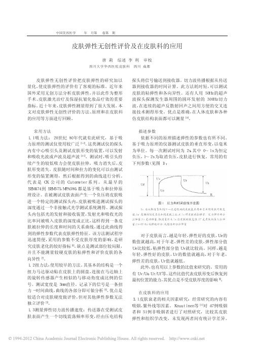
Shear-wave polarization analysis has been performed on data from twelve earthquakes recorded in central Italy. These data are part of a set of high quality seismograms recorded by a three-component digital network installed in Abruzzo region after a Ms = 5.8 earthquake on 7 May 1984. Analysis performed on 2 to 6 Hz bandpass-filtered seismograms reveals shear-wave splitting. In order to determine the direction for which the time separation between the two split S waves is maximum, the horizontal traces are rotated in the range 10 to 90 ° with steps of 10 ° . At each step the cross-correlation between the two shear waves and the time separation is estimated. The azimuth of 50°N yields the highest correlation coefficient and the maximum time separation of about 0.09 sec. This direction and the orthogonal to it represent axes of minimum and maximum shear-wave velocity respectively. If the time delay is distributed over the whole hypocenter-seismic station path, the maximum variation in velocity is at least 1.4 per cent. The theoretical linear polarization of particle motion at the source is verifi seismograms for the anisotropic propagation effect. A distribution of vertical cracks aligned in the direction 140°N may explain the observed anisotropy. The stress field deduced from the focal mechanism of the Abruzzo earthquake is compatible with this hypothetical crack distribution.
Bulletin of the Seismological Society of America, Vol. 79, No. 6, pp. 1905-1912, December 1989
EVIDENCE OF SHEAR-WAVE ANISOTROPY IN T H E U P P E R CRUST OF CENTRAL ITALY BY G. IANNACCONE AND A. DESCHAMPS ABSTRACT
1906
G. IANNACCONE AND A. DESCHAMPS
The aim of this paper is to present the first results of seismic shear-wave polarization which show evidence of anisotropy in the upper crust of central Italy. DATA Just after an earthquake of Ms -- 5.8 occurred on 7 May 1984 in the Abruzzo region a digital seismic network composed of seven three-component short-period stations was installed in the epicentral area. This network operated for ten days in the framework of a scientific cooperative program between the Osservatorio Vesuviano and the University of Wisconsin. The stations that operated in triggering mode are wide dynamic range (106 db) instruments equipped with three 1 Hz geophones. The seismic signal was digitized at a rate of 100 sample/sec and stored on field tapes in 30 sec records. The amplitude response curve is almost flat in velocity between 2 and 25 Hz. About 1000 events were recorded by at least four stations of the network dur