An ordinary differential equation model for the multistep transformation
常微分方程的英文
常微分方程的英文Ordinary Differential EquationsIntroductionOrdinary Differential Equations (ODEs) are mathematical equations that involve derivatives of unknown functions with respect to a single independent variable. They find application in various scientific disciplines, including physics, engineering, economics, and biology. In this article, we will explore the basics of ODEs and their importance in understanding dynamic systems.ODEs and Their TypesAn ordinary differential equation is typically represented in the form:dy/dx = f(x, y)where y represents the unknown function, x is the independent variable, and f(x, y) is a given function. Depending on the nature of f(x, y), ODEs can be classified into different types.1. Linear ODEs:Linear ODEs have the form:a_n(x) * d^n(y)/dx^n + a_(n-1)(x) * d^(n-1)(y)/dx^(n-1) + ... + a_1(x) * dy/dx + a_0(x) * y = g(x)where a_i(x) and g(x) are known functions. These equations can be solved analytically using various techniques, such as integrating factors and characteristic equations.2. Nonlinear ODEs:Nonlinear ODEs do not satisfy the linearity condition. They are generally more challenging to solve analytically and often require the use of numerical methods. Examples of nonlinear ODEs include the famous Lotka-Volterra equations used to model predator-prey interactions in ecology.3. First-order ODEs:First-order ODEs involve only the first derivative of the unknown function. They can be either linear or nonlinear. Many physical phenomena, such as exponential decay or growth, can be described by first-order ODEs.4. Second-order ODEs:Second-order ODEs involve the second derivative of the unknown function. They often arise in mechanical systems, such as oscillators or pendulums. Solving second-order ODEs requires two initial conditions.Applications of ODEsODEs have wide-ranging applications in different scientific and engineering fields. Here are a few notable examples:1. Physics:ODEs are used to describe the motion of particles, fluid flow, and the behavior of physical systems. For instance, Newton's second law of motion can be formulated as a second-order ODE.2. Engineering:ODEs are crucial in engineering disciplines, such as electrical circuits, control systems, and mechanical vibrations. They allow engineers to model and analyze complex systems and predict their behavior.3. Biology:ODEs play a crucial role in the study of biological dynamics, such as population growth, biochemical reactions, and neural networks. They help understand the behavior and interaction of different components in biological systems.4. Economics:ODEs are utilized in economic models to study issues like market equilibrium, economic growth, and resource allocation. They provide valuable insights into the dynamics of economic systems.Numerical Methods for Solving ODEsAnalytical solutions to ODEs are not always possible or practical. In such cases, numerical methods come to the rescue. Some popular numerical techniques for solving ODEs include:1. Euler's method:Euler's method is a simple numerical algorithm that approximates the solution of an ODE by using forward differencing. Although it may not provide highly accurate results, it gives a reasonable approximation when the step size is sufficiently small.2. Runge-Kutta methods:Runge-Kutta methods are higher-order numerical schemes for solving ODEs. They give more accurate results by taking into account multiple intermediate steps. The most commonly used method is the fourth-order Runge-Kutta (RK4) algorithm.ConclusionOrdinary Differential Equations are a fundamental tool for modeling and analyzing dynamic systems in various scientific and engineering disciplines. They allow us to understand the behavior and predict the evolution of complex systems based on mathematical principles. With the help of analytical and numerical techniques, we can solve and interpret different types of ODEs, contributing to advancements in science and technology.。
ordinary的意思用法总结

ordinary的意思用法总结ordinary一般的,平常的,一般的,平凡的的意思。
那你们想知道ordinary的用法吗?今日我给大家带来了ordinary的用法 ,期望能够帮忙到大家,一起来学习吧。
ordinary的意思adj. 一般的,平常的,一般的,平凡的ordinary用法ordinary可以用作形容词ordinary的基本意思是“一般的”“平常的”“一般的”“平凡的”。
指与一般事物的性质标准相同,强调“平常”而无高超奇怪之处。
ordinary在句中可用作定语,也可用作表语,间或也可用作宾语补足语。
ordinary没有比较级和最高级。
ordinary用作形容词的用法例句I just want an ordinary car without the frills.我只要一辆没有多余装饰的一般汽车。
Now electrical appliances have entered into ordinary families.现在家用电器已经步入一般家庭。
It was an ordinary lunch of soup and a sandwich.那是一顿平淡的午餐:一份汤,一份三明治。
ordinary用法例句1、It was just an ordinary voice, but he sang in tune.他声音很一般,但唱得都在调子上。
2、Ordinary people are at the mercy of faceless bureaucrats.一般人的命运任凭那些平凡刻板的官僚们摆布。
3、This Human Rights Act is enforceable in the ordinary courts.这项《人权法案》适用于一般法庭。
ordinary词组 | 习惯用语in ordinary (职务等)常任的;(待修的船只等)闲搁着的ordinary people 一般人,一般人out of the ordinary 不平常的ordinary life 正常寿命;常规生命ordinary differential equation 常微分方程ordinary day 平常的一天;[地磁]平常日ordinary course 正常贸易;常规过程ordinary temperature 常温,室温ordinary portland cement 一般硅酸盐水泥ordinary workers 一般劳动者ordinary income 一般收入ordinary mail n. 平信ordinary share 一般股ordinary light 寻常光;一般光线ordinary level 一般程度的;(英)一般级考试(等于O leve)ordinary goods 一般品;一般货物ordinary quality 中等质量ordinary 英语例句库1.The royal family is insulated from many of the difficulties faced by ordinary people.王室成员都毋须应付平民所面临的很多困难。
Ordinary differential equations with only entire solutions

a rX iv:mat h /97621v1[mat h.CV]6J u n1997ORDINARY DIFFERENTIAL EQUATIONS WITH ONLY ENTIRE SOLUTIONS ERIK ANDERS ´EN Abstract.We prove necessary and sufficient conditions for a system ˙z i =z i p i (z )(p i a polynomial)to have only entire analytic functions as solutions. 1.preliminaries We will need the following elementary facts from Nevanlinna theory.For any entire function of one complex variable f (z )we set m (r,f )=1a and T (r,f )=m (r,f )+N (r,f ).In the definition of N ,the sum is taken over all poles a of f ,with regard to multiplicity.The function T (r,f )is called the Nevanlinna characteristic of f .The following properties are easily verified.T (r,f 1+f 2)≤T (r,f 1)+T (r,f 2)+O (1)T (r,f 1f 2)≤T (r,f 1)+T (r,f 2),T (r,f d )=dT (r,f ).(1)Here and in the sequel,the estimates O (g )and o (g )are as r →∞.The first fundamental theorem of Nevanlinna theory says that T (r,1/f )=T (r,f )+O (1).We also have the Lemma of the logarithmic derivative (LLD),m (r,f ′/f )=o excl (T (r,f )).Here o excl means that the estimate holds outside a set of finite measure.We also use the corresponding notation O excl .From LLD and the preceding inequalities it follows thatm (r,f (k ))≤(1+o excl (1)))T (r,f )(2)m (r,f (k )/f )=o excl (T (r,f ))(3)2ERIK ANDERS´ENfor all positive integers k.2.Borel’s TheoremWe need a version of a theorem named after Borel,which is classical,but which is proved here since I have not found a good reference to it.We call an entire holomorphic function a unit if it has no zeros.Theorem1.Let f be an entire function and u1,u2,...,u n be units satis-fyingu i=f.(4) Then one of the following cases holds.1.T(r,u i)=O excl(T(r,f)+1)for all i.2.Some subsum i∈I u i=0.Proof.The proof is by induction.If n=1then Case1holds automatically so there is nothing to prove.We assume that the theorem holds for sums with less than n terms.If we differentiate(4)we getu(j)iORDINARY DIFFERENTIAL EQUATIONS WITH ONLY ENTIRE SOLUTIONS3(a)T(v i,r)=O excl(T(1,r)+1)=O excl(1)for all i.Then all v i areconstant and u i=a i u1for some a i.The sum(4)now becomes( a i+1)u1=f.If a i+1=0,then f=0and we haveCase2;otherwise,u1is proportional to f and then all u i are alsoproportional to f.We then have Case1.(b) i∈I v i=0for some set I.Then i∈I c i u i=0and this sum isshorter than(5).This is a contradiction.3.Differential equationsTheorem2.Let p i be Laurent-polynomials and˙z i=z i p i(z)z i(0)=c i1≤i≤n(7) be an ordinary differential equation such that for all c in some open set all components of the solutions are units.Thenp(Z)=n−1k=1u kθk(M(k))+u0.(8)Here u k∈C n,M(k)∈C[Z,Z−1]k is defined by M(n)=Z andM(k−1)i= M(k)j a(k)ij for k=n,...,2,(9) where a(k)are(k−1,k)-matrices satisfying a(k)...a(n)u k=0andθk are Laurent-polynomials.Conversely,any system of the form(8)has only entire solutions,and all components are either units or identically zero.The proof needs a lemma.We write p(Z)=(p1(Z),...,p n(Z)),p(Z)= pαZαand pα=(pα,1,...,pα,n).We let Dg denote(˙g1/g1,...,˙g n/g n).Let S be the set of meromorphic functions satisfying T(r,f)=o excl(T(r,z1)+···+T(r,z n)+1).Lemma1.Let M be the multiplicative module generated by of N={Zα: pα,i=0for some i}.Then dim M<n.Proof.Choose c so that α∈A pα,i cα=0for all non-zero subpolynomials and all indices i,and so that all components of the solution are units.Let z(t) be the solution with z(0)=c.Apply Borel’s theorem to pα,i zα=˙z i/z i. Because of our choice of initial condition,Case2does not hold.Therefore, N⊂S.It follows from the rules(1)that M⊂S.Assume that the dimension of M is n.Then for each i there is d i such that z d i∈M⊂S.Again by(1),z i∈S for each i.This is impossible and therefore the dimension is less than n.Proof of Theorem2.The proof is by induction.The theorem holds if n=1, so we assume that it holds for systems with smaller number of variables.We first prove the necessity of(8).Assume that(7)has only entire solutions. By Lemma1we can write p(Z)=f(M),where M=(M1,...,M l)and M i= Z a ij j,and l<n.We may assume that a=(a ij)has full rank since4ERIK ANDERS ´ENwe can otherwise drop some variables M i .If l <n −1we can complete a to an (n −1,n )-matrix of full rank,so we assume that l =n −1.Set m i = z a ij j .Then Dz =p (z )=f (m )and logarithmic differentiation gives Dm =af (m ).By induction,af (M )=n −2 k =1v k θk (M (k ))+v 0,where M (k )are given by (9)for k =n −1,...,2and a (k )...a (n −1)v k =0.Since a is surjective v k =au k for some u k sof (M )−n −2 k =1v k θk (M (k ))−v 0∈Ker a.Since this kernel is one-dimensional we havef (M )=u n −1θn −1(M )+n −2 k =1u k θk (M (k ))+u 0for some u n −1∈Ker a ⊂C n and some Laurent-polynomial θn −1.If we set M (n −1)=M and a (n −1)=a the first half of the theorem is proved.If the system is of form (8)then we get as above thatDm =a(n )(n −1 k =1u k θk (m (k ))+u 0)=n −2 k =1a (n )u k θk (m (k ))+a (n )u 0since a (n )u n =0by assumption.By induction,this system has only entire solutions m (t ).An integration of ˙z i /z i =f i (m (t ))now proves the rest of the theorem.Remark .Although the form (8),(9)is complicated,the proof gives an extremely simple recursive algorithm to determine if all solutions to a system are entire.First compute the multiplicative span of all Z αsuch that p α,i =0for some i .If this is the whole space,the system does have non-entire solutions.Otherwise,let M i be a basis for this space,and express p (Z )=f (M )in terms of this basis.Differentiate logarithmically to get a new equation Dm =af (m )(with notations as in the theorem).The original system has only entire solutions if and only if this new system has.Remark .If the polynomials p i are genuine polynomials,it is immediately clear that all components of any solution are either zero-free or identically zero.Corollary 1.All complete polynomial vector fields on (C ∗)n are of the form(7)with p satisfying (8).ORDINARY DIFFERENTIAL EQUATIONS WITH ONLY ENTIRE SOLUTIONS5 Corollary2.All complete polynomial vectorfields on(C∗)n preserve the volume form dz i/z i.Proof.The proof is again by induction.We computedz i =d˙z i z i−˙z i dz iz2i=d(p i(z)).This shows in particular that the result holds for n=1.Also,we compute dz i= i dz1dt dz i z n= i z i∂p i z i .We use the notation of the proof of the theorem and in particular the result that p(z)=f(m)and Dm=af(m).We have to prove that z i∂p i/∂z i(z)= 0,so we computei z i∂f i∂m j∂m j∂m j m j a ji∂m jm j a ji= j∂(af)j。
Differential equation
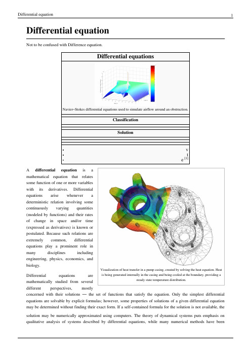
Differential equationNot to be confused with Difference equation.Stokes differential equations used to simulate airflow around an obstruction.ClassificationSolutionVisualization of heat transfer in a pump casing, created by solving the heat equation. Heat is being generated internally in the casing and being cooled at the boundary, providing a steady state temperature distribution.A differential equation is amathematical equation that relatessome function of one or more variableswith its derivatives. Differentialequations arise whenever adeterministic relation involving somecontinuously varying quantities(modeled by functions) and their ratesof change in space and/or time(expressed as derivatives) is known orpostulated. Because such relations areextremely common, differentialequations play a prominent role inmany disciplines includingengineering, physics, economics, andbiology.Differential equations aremathematically studied from severaldifferent perspectives, mostlyconcerned with their solutions — the set of functions that satisfy the equation. Only the simplest differential equations are solvable by explicit formulas; however, some properties of solutions of a given differential equation may be determined without finding their exact form. If a self-contained formula for the solution is not available, the solution may be numerically approximated using computers. The theory of dynamical systems puts emphasis on qualitative analysis of systems described by differential equations, while many numerical methods have beendeveloped to determine solutions with a given degree of accuracy.ExampleFor example, in classical mechanics, the motion of a body is described by its position and velocity as the time value varies. Newton's laws allow one (given the position, velocity, acceleration and various forces acting on the body) to express these variables dynamically as a differential equation for the unknown position of the body as a function of time.In some cases, this differential equation (called an equation of motion) may be solved explicitly.An example of modelling a real world problem using differential equations is the determination of the velocity of a ball falling through the air, considering only gravity and air resistance. The ball's acceleration towards the ground is the acceleration due to gravity minus the acceleration due to air resistance. Gravity is considered constant, and air resistance may be modeled as proportional to the ball's velocity. This means that the ball's acceleration, which is a derivative of its velocity, depends on the velocity (and the velocity depends on time). Finding the velocity as a function of time involves solving a differential equation and verifying its validity.Directions of studyThe study of differential equations is a wide field in pure and applied mathematics, physics, and engineering. All of these disciplines are concerned with the properties of differential equations of various types. Pure mathematics focuses on the existence and uniqueness of solutions, while applied mathematics emphasizes the rigorous justification of the methods for approximating solutions. Differential equations play an important role in modelling virtually every physical, technical, or biological process, from celestial motion, to bridge design, to interactions between neurons. Differential equations such as those used to solve real-life problems may not necessarily be directly solvable, i.e. do not have closed form solutions. Instead, solutions can be approximated using numerical methods.Mathematicians also study weak solutions (relying on weak derivatives), which are types of solutions that do not have to be differentiable everywhere. This extension is often necessary for solutions to exist.The study of the stability of solutions of differential equations is known as stability theory.NomenclatureThe theory of differential equations is well developed and the methods used to study them vary significantly with the type of the equation.Ordinary and partial•An ordinary differential equation (ODE) is a differential equation in which the unknown function (also known as the dependent variable) is a function of a single independent variable. In the simplest form, the unknown function is a real or complex valued function, but more generally, it may be vector-valued or matrix-valued: this corresponds to considering a system of ordinary differential equations for a single function.Ordinary differential equations are further classified according to the order of the highest derivative of the dependent variable with respect to the independent variable appearing in the equation. The most important cases for applications are first-order and second-order differential equations. For example, Bessel's differential equation(in which y is the dependent variable) is a second-order differential equation. In the classical literature a distinction is also made between differential equations explicitly solved with respect to the highest derivative and differential equations in an implicit form. Also important is the degree, or (highest) power, of the highest derivative(s) in the equation (cf. : degree of a polynomial). A differential equation is called a nonlinear differential equation if its degree is not one (a sufficient but unnecessary condition).• A partial differential equation (PDE) is a differential equation in which the unknown function is a function of multiple independent variables and the equation involves its partial derivatives. The order is defined similarly to the case of ordinary differential equations, but further classification into elliptic, hyperbolic, and parabolic equations, especially for second-order linear equations, is of utmost importance. Some partial differentialequations do not fall into any of these categories over the whole domain of the independent variables and they are said to be of mixed type.Linear and non-linearBoth ordinary and partial differential equations are broadly classified as linear and nonlinear.• A differential equation is linear if the unknown function and its derivatives appear to the power 1 (products of the unknown function and its derivatives are not allowed) and nonlinear otherwise. The characteristic property of linear equations is that their solutions form an affine subspace of an appropriate function space, which results in much more developed theory of linear differential equations. Homogeneous linear differential equations are a further subclass for which the space of solutions is a linear subspace i.e. the sum of any set of solutions or multiples of solutions is also a solution. The coefficients of the unknown function and its derivatives in a linear differential equation are allowed to be (known) functions of the independent variable or variables; if these coefficients are constants then one speaks of a constant coefficient linear differential equation.•There are very few methods of solving nonlinear differential equations exactly; those that are known typically depend on the equation having particular symmetries. Nonlinear differential equations can exhibit verycomplicated behavior over extended time intervals, characteristic of chaos. Even the fundamental questions of existence, uniqueness, and extendability of solutions for nonlinear differential equations, and well-posedness of initial and boundary value problems for nonlinear PDEs are hard problems and their resolution in special cases is considered to be a significant advance in the mathematical theory (cf. Navier–Stokes existence and smoothness).However, if the differential equation is a correctly formulated representation of a meaningful physical process, then one expects it to have a solution.Linear differential equations frequently appear as approximations to nonlinear equations. These approximations are only valid under restricted conditions. For example, the harmonic oscillator equation is an approximation to the nonlinear pendulum equation that is valid for small amplitude oscillations (see below).ExamplesIn the first group of examples, let u be an unknown function of x, and c and ω are known constants.•Inhomogeneous first-order linear constant coefficient ordinary differential equation:•Homogeneous second-order linear ordinary differential equation:•Homogeneous second-order linear constant coefficient ordinary differential equation describing the harmonic oscillator:•Inhomogeneous first-order nonlinear ordinary differential equation:•Second-order nonlinear (due to sine function) ordinary differential equation describing the motion of a pendulum of length L:In the next group of examples, the unknown function u depends on two variables x and t or x and y.•Homogeneous first-order linear partial differential equation:•Homogeneous second-order linear constant coefficient partial differential equation of elliptic type, the Laplace equation:•Third-order nonlinear partial differential equation, the Korteweg–de Vries equation:Related concepts• A delay differential equation (DDE) is an equation for a function of a single variable, usually called time, in which the derivative of the function at a certain time is given in terms of the values of the function at earlier times.• A stochastic differential equation (SDE) is an equation in which the unknown quantity is a stochastic process and the equation involves some known stochastic processes, for example, the Wiener process in the case of diffusion equations.• A differential algebraic equation (DAE) is a differential equation comprising differential and algebraic terms, given in implicit form.Connection to difference equationsSee also: Time scale calculusThe theory of differential equations is closely related to the theory of difference equations, in which the coordinates assume only discrete values, and the relationship involves values of the unknown function or functions and values at nearby coordinates. Many methods to compute numerical solutions of differential equations or study the properties of differential equations involve approximation of the solution of a differential equation by the solution of a corresponding difference equation.Universality of mathematical descriptionMany fundamental laws of physics and chemistry can be formulated as differential equations. In biology and economics, differential equations are used to model the behavior of complex systems. The mathematical theory of differential equations first developed together with the sciences where the equations had originated and where the results found application. However, diverse problems, sometimes originating in quite distinct scientific fields, may give rise to identical differential equations. Whenever this happens, mathematical theory behind the equations can be viewed as a unifying principle behind diverse phenomena. As an example, consider propagation of light and sound in the atmosphere, and of waves on the surface of a pond. All of them may be described by the same second-order partial differential equation, the wave equation, which allows us to think of light and sound as forms of waves, much like familiar waves in the water. Conduction of heat, the theory of which was developed by Joseph Fourier, is governed by another second-order partial differential equation, the heat equation. It turns out that many diffusion processes, while seemingly different, are described by the same equation; the Black–Scholes equation in finance is, for instance, related to the heat equation.Notable differential equationsPhysics and engineering•Newton's Second Law in dynamics (mechanics)•Euler–Lagrange equation in classical mechanics•Hamilton's equations in classical mechanics•Radioactive decay in nuclear physics•Newton's law of cooling in thermodynamics•The wave equation•Maxwell's equations in electromagnetism•The heat equation in thermodynamics•Laplace's equation, which defines harmonic functions•Poisson's equation•Einstein's field equation in general relativity•The Schrödinger equation in quantum mechanics•The geodesic equation•The Navier–Stokes equations in fluid dynamics•The Diffusion equation in stochastic processes•The Convection–diffusion equation in fluid dynamics•The Cauchy–Riemann equations in complex analysis•The Poisson–Boltzmann equation in molecular dynamics•The shallow water equations•Universal differential equation•The Lorenz equations whose solutions exhibit chaotic flow.Biology•Verhulst equation – biological population growth•von Bertalanffy model – biological individual growth•Lotka–Volterra equations – biological population dynamics•Replicator dynamics – found in theoretical biology•Hodgkin–Huxley model – neural action potentialsEconomics•The Black–Scholes PDE•Exogenous growth model•Malthusian growth model•The Vidale–Wolfe advertising modelReferences•P. Abbott and H. Neill, Teach Yourself Calculus, 2003 pages 266-277•P. Blanchard, R. L. Devaney, G. R. Hall, Differential Equations, Thompson, 2006• E. A. Coddington and N. Levinson, Theory of Ordinary Differential Equations, McGraw-Hill, 1955• E. L. Ince, Ordinary Differential Equations, Dover Publications, 1956•W. Johnson, A Treatise on Ordinary and Partial Differential Equations[2], John Wiley and Sons, 1913, in University of Michigan Historical Math Collection [3]• A. D. Polyanin and V. F. Zaitsev, Handbook of Exact Solutions for Ordinary Differential Equations (2nd edition), Chapman & Hall/CRC Press, Boca Raton, 2003. ISBN 1-58488-297-2.•R. I. Porter, Further Elementary Analysis, 1978, chapter XIX Differential Equations•Teschl, Gerald (2012). Ordinary Differential Equations and Dynamical Systems[4]. Providence: American Mathematical Society. ISBN 978-0-8218-8328-0.• D. Zwillinger, Handbook of Differential Equations (3rd edition), Academic Press, Boston, 1997.[1]/w/index.php?title=Template:Differential_equations&action=edit[2]/cgi/b/bib/bibperm?q1=abv5010.0001.001[3]/u/umhistmath/[4]http://www.mat.univie.ac.at/~gerald/ftp/book-ode/External links•Lectures on Differential Equations (/courses/mathematics/18-03-differential-equations-spring-2010/video-lectures/) MIT Open CourseWare Videos•Online Notes / Differential Equations (/classes/de/de.aspx) Paul Dawkins, Lamar University•Differential Equations (/diffeq/diffeq.html), S.O.S. Mathematics•Differential Equation Solver (/tools/differential_equation_solver/) Java applet tool used to solve differential equations.•Introduction to modeling via differential equations (/mat/u-u/en/ differential_equations_intro.htm) Introduction to modeling by means of differential equations, with critical remarks.•Mathematical Assistant on Web (http://user.mendelu.cz/marik/maw/index.php?lang=en&form=ode) Symbolic ODE tool, using Maxima•Exact Solutions of Ordinary Differential Equations (http://eqworld.ipmnet.ru/en/solutions/ode.htm)•Collection of ODE and DAE models of physical systems (/research/models.htm) MATLAB models•Notes on Diffy Qs: Differential Equations for Engineers (/diffyqs/) An introductory textbook on differential equations by Jiri Lebl of UIUC•Khan Academy Video playlist on differential equations (/math/ differential-equations) Topics covered in a first year course in differential equations.•MathDiscuss Video playlist on differential equations (/category/courses/ solutions-differential-equations/homogeneous-linear-systems/)Article Sources and Contributors8Article Sources and ContributorsDifferential equation Source: /w/index.php?oldid=610771276 Contributors: 17Drew, After Midnight, Ahoerstemeier, Alarius, Alfred Centauri, Amahoney, AndreiPolyanin, Andres, AndrewHowse, Andycjp, Andytalk, AngryPhillip, Anonymous Dissident, Antoni Barau, Antonius Block, Anupam, Apmonitor, Arcfrk, Asdf39, Asyndeton, Attilios,Babayagagypsies, Baccala@, Baccyak4H, Bejohns6, Bento00, Berland, Bidabadi, Bigusbry, BillyPreset, Bob.v.R, Bolatbek, Brandon, Bryanmcdonald, Btyner, Bygeorge2512,Callumds, Charles Matthews, Christian75, Chtito, Cispyre, Cmprince, Coginsys, ConMan, Cxz111, Cybercobra, DAJF, Danski14, Dbroadwell, Ddxc, Delaszk, DerHexer, Dewritech, Difu Wu, Djordjes, DominiqueNC, Donludwig, Dpv, Dr sarah madden, Drmies, DroEsperanto, Duoduoduo, Dysprosia, EconoPhysicist, Elwikipedista, Epicgenius, EricBright, Erin.Annette.Brown,Estudiarme, F=q(E+v^B), Fintor, Fioravante Patrone, Fioravante Patrone en, Flameturtle, Friend of the Facts, FutureTrillionaire, Gabrielleitao, Gandalf61, Gauss, Genedronek, Geni, Giftlite,GoingBatty, Gombang, Grenavitar, Haham hanuka, Hamiltondaniel, Harry, Haruth, Haseeb Jamal, Heikki m, Holmes1900, Ilya Voyager, Iquseruniv, Iulianu, Izodman2012, J arino, J.delanoy, Ja 62, Jak86, JamesBWatson, Jao, Jarble, Jauhienij, Jayden54, Jeancey, Jersey Devil, Jim Sukwutput, Jim.belk, Jim.henderson, JinJian, Jitse Niesen, JohnOwens, Johndoeisnotmyname, JorisvS,Julesd, K-UNIT, Kayvan45622, KeithJonsn, Kensaii, Khalid Mahmood, Klaas van Aarsen, Kr5t, Krushia, LOL, Lambiam, Lavateraguy, Lethe, LibLord, Linas, Lumos3, Madmath789, Mandarax, Mankarse, MarSch, Martastic, Martynas Patasius, Maschen, Math.geek3.1415926, Matqkks, Mattmnelson, Maurice Carbonaro, Maxis ftw, Mazi, McVities, Mduench, Mets501, Mh, MichaelHardy, Mindspillage, MisterSheik, Mohan1986, Mossaiby, Mpatel, MrOllie, Mtness, Mysidia, Nik-renshaw, Nkayesmith, Norm mit, Okopecz, Oleg Alexandrov, Opelio, Pahio, Parusaro, Paul August, Paul Matthews, Paul Richter, PavelSolin, Pgk, Phoebe, Pine, Pinethicket, Pratyya Ghosh, PseudoSudo, Qwerty Binary, Qzd800, R'n'B, Rama's Arrow, Randomguess, Reallybored999, RexNL, Reyk, RichMorin, Robin S, Romansanders, Rosasco, Ruakh, SDC, SFC9394, SakeUPenn, Salix alba, Sam Staton, Sampathsris, Sardanaphalus, Senoreuchrestud, Silly rabbit, Siroxo,Skakkle, Skypher, SmartPatrol, Snowjeep, Spirits in the Material, Starwiz, Suffusion of Yellow, Sverdrup, Symane, TVBZ28, TYelliot, Tannkrem, Tbhotch, Tbsmith, TexasAndroid, Tgeairn, The Hybrid, The Thing That Should Not Be, Timelesseyes, Tranum1234567890, Tsirel, Tuseroni, User A1, Vanished User 0001, Vishwanathnm, Vthiru, Waffleguy4, Waldir, Waltpohl, Wavelength, Wclxlus, Wihenao, Willtron, Winterheart, Wsears, XJaM, Yafujifide, Zepterfd, ﺪﺟﺎﺳ ﺪﺠﻣﺍ ﺪﺟﺎﺳ, 363 anonymous editsImage Sources, Licenses and ContributorsFile:Airflow-Obstructed-Duct.png Source: /w/index.php?title=File:Airflow-Obstructed-Duct.png License: Public Domain Contributors: Original uploader was User A1 at en.wikipediaFile:Elmer-pump-heatequation.png Source: /w/index.php?title=File:Elmer-pump-heatequation.png License: Creative Commons Attribution-Sharealike 3.0Contributors: Christian1985, Crimerob, Kri, User A1, 2 anonymous editsLicenseCreative Commons Attribution-Share Alike 3.0///licenses/by-sa/3.0/。
仿射非线性系统状态方程的任意阶近似解

仿射非线性系统状态方程的任意阶近似解曹少中1,2) 刘贺平2) 涂序彦2)1)北京印刷学院信息与机电工程学院,北京102600 2)北京科技大学信息工程学院,北京100083摘 要 针对典型的仿射非线性系统,采用常微分方程理论对其进行求解.首先将系统在平衡点附近进行展开,求得其齐次方程的解,然后利用常数变易法将非线性微分方程变为等价的第二类非线性Volterra 积分方程.采用逐次逼近法,求得任意阶近似解,并证明解的收敛性.关键词 非线性系统;状态方程;常微分方程;Volterra 积分方程;逐次逼近法;近似解分类号 TP 273Any order approximate solution of the state equation for an aff ine nonlinear sys 2temCA O S haoz hong1,2),L IU Heping2),TU X uyan2)1)College of Information &Mechanical Engineering ,Beijing Institute of Graphic Communication ,Beijing 102600,China 2)School of Information Engineering ,University of Science and Technology Beijing ,Beijing 100083,ChinaABSTRACT The state equation of an typical affine nonlinear system was solved with the ordinary differential equation theory.By utilizing the expansion expression of equilibrium point of the system ,the homogeneous equation ’s solution was obtained ,and then the nonlinear differential equation was equivalent to its nonlinear Volterra ’s integral equation of the second kind by the constant variation method.Any order approximate solution of the equation was presented ,and its convergence was mathematically proved by the succes 2sive approximation method.KE Y WOR DS nonlinear system ;state equation ;ordinary differential equation ;Volterra ’s integral equation ;successive approxima 2tion method ;approximate solution收稿日期:2007204212 修回日期:2007207225基金项目:国家自然科学基金资助项目(No.60374032,No.60673101);北京市教育委员会科技发展计划面上项目(No.KM200810015003);北京市属市管高等学校人才强教计划资助项目(No.TXM2007-014223-044661);北京印刷学院引进人才科技研究项目(No.0917*******)作者简介:曹少中(1965—),男,副教授,博士,E 2mail :cszh6502@ 由于非线性控制理论的复杂性,人们在研究过程中,逐渐从以常微分方程理论作为主要数学工具,转到以拓扑学、微分几何等现代数学工具为主,从而在近几十年,使得非线性控制理论特别是对仿射非线性系统的研究取得了长足的发展[1-4].以微分几何为主要工具发展起来的精确线性化方法,为解决仿射非线性控制系统的分析与综合问题提供了强有力的手段.由于精确线性化方法必须满足苛刻的条件,且结构复杂,除了某些具有特殊结构(如三角形结构)的系统外,往往很难得到所需的非线性变换;因此研究非线性系统的近似处理方法具有相当的理论与应用意义,近年来也一直同样受到人们的高度重视.近似线性化方法[5-7]被证明在平衡点的某一邻域内是有效的,误差可以接受,所以广泛地应用于实际系统中.但是这些近似线性化方法误差较大,在精度要求较高的情况下不能满足要求.本文拟采用传统的常微分方程和积分方程理论,给出一种求解仿射非线性系统的近似线性化方法,本方法可使结果达到任意阶近似.本文采用传统的常微分方程和积分方程理论,对仿射非线性系统进行求解.首先将系统在平衡点x =0附近进行展开,求得其齐次方程的解;然后利用常数变易法将非线性微分方程变为等价的第二类非线性Volterra 积分方程.采用逐次逼近法,求得任意阶近似解,并证明解的收敛性.第30卷第6期2008年6月北京科技大学学报Journal of U niversity of Science and T echnology B eijingV ol.30N o.6Jun.20081 仿射非线性系统的任意阶近似解一个有限n 维的控制系统可以描述为:x ・=f (x ,u )y =h (x ,u) x ∈M ,u ∈U(1)其中,M 是一个n 维流形,U 是容许控制集合.系统(1)的一个常用的特殊情况是仿射非线性系统,它是对状态x 非线性而对u 是线性的.实际上,仿射非线性系统可由如下方程描述[1-2]:x ・=f (x )+g (x )uy =h (x) x ∈M ,u ∈U (2)其中,f (x )=(f 1(x ),f 2(x ),…,f n (x ))T,g (x )=g 11(x )g 12(x )…g 1m (x)g 21(x )g 22(x )…g 2m (x )…g n 1(x )g n 2(x )…g nm (x ),x =(x 1,x 2,…,x n )T为状态向量,u =(u 1,u 2,…,u m )T为控制向量,y =(y 1,y 2,…,y p )T为输出向量,h (x )=(h 1(x ),h 2(x ),…,h p (x ))T为输出函数向量.通常f 是光滑向量场,并且f (0)=0在h (x )=(h 1(x ),h 2(x ),…,h p (x ))T中的h i (x )满足h i (0)=0(i =1,2,…,p ),且它们是光滑的,另外在系统(2)中的g ij (x )(i =1,2,…,n ;j =1,2,…,m )也是M 上光滑的向量场.易知,x =0是该系统的平衡点(设u =0).将f (x )和g (x )在平衡点x =0(u =0)附近展开有:f i (x )=∑nj =1aij(t )x j +∑nj 1=1∑nj 2=1aij 1j 2(t )x j 1x j 2+∑nj 1=1∑nj 2=1∑nj 3=1aij 1j 2j 3(t )x j 1x j 2x j 3+…+∑nj 1=1∑nj 2=1…∑nj k=1aij 1j 2…j k(t )x j 1x j 2x j 3…x j k+ (3)令Ψi (x (t ),t )=∑nj 1=1∑nj 2=1aij 1j 2(t )x j 1x j 2+∑nj 1=1∑nj 2=1∑nj 3=1aij 1j 2j 3(t )x j 1x j 2x j 3+…+∑nj 1=1∑nj 2=1…∑nj k=1a ij 1j 2...j k (t )x j 1x j 2...x j k + (4)即为式(3)中的高次项部分,于是式(3)可写为:f i (x )=∑nj =1aij(t )x j +Ψi (x (t ),t )(5)同理,g ij (x )可写为线性和非线性两部分:g ij (x )=b ij (t )+G i (x (t ),t )(6)其中,b ij (t )与x 无关,G (x (t ),t )为高次项部分.将式(5)及(6)代入方程(2),则原方程变为下面的形式:x ・(t )=A (t )x (t )+B (t )u (t )+Ψ(x (t ),t )+G (x (t ),t )u (t )(7)其中,A (t )=a 11(t )a 12(t )…a 1n (t )a 21(t )a 22(t )…a 2n (t )…a n 1(t )a n 2(t )…a nn (t ),B (t )=b 11(t )b 12(t )…b 1m (t )b 21(t )b 22(t )…b 2m (t )…b n 1(t )b n 2(t )…b nm (t ),Ψ(x (t ),t )=(Ψ1(x (t ),t ),Ψ2(x (t ),t ),…Ψn (x (t ),t ))T,G (x (t ),t )=G 11(x (t ),t )G 12(x (t ),t )…G 1m (x (t ),t )G 21(x (t ),t )G 22(x (t ),t )…G 2m (x (t ),t )…G n 1(x (t ),t )G n 2(x (t ),t )…G nm (x (t ),t ).首先求解式(7)的齐次方程,x ^(t )=A (t )x (t )(8)初始条件为x (t =0)=x (0).该方程早已被人们采用Picad 递归积分法或时变距阵指数法分别给出如下形式的解:x (t )=R (t )x (0)(9)R (t )=I +∫tA (t 1)d t1+∫t 0∫t 1A (t 1)A (t 2)d t 2d t 1+…+∫t0∫t 10…∫t n-1A (t 1)A (t 2)…A (t n )d t n d t n -1…d t 2d t 1+…(10)或R (t )=exp∫tA (τ)d τ(11)・196・第6期曹少中等:仿射非线性系统状态方程的任意阶近似解在求得齐次方程解的基础上,采用常数变易法将非线状态方程(7)变为等价的积分方程.设式(7)的解的形式为:x (t )=R (t )C (t )(12)其中,C (t )为待求函数列向量,根据R (t )的初始条件R (0)=I (n ×n 单位矩阵),可知C (t )的初始条件为C (0)=x (0).把式(12)代入式(7),有d R (t )d t C (t )+R (t )d C (t )d t=A (t )R (t )C (t )+B (t )u (t )+Ψ(x (t ),t )+G (x (t ),t )u (t ),利用d R (t )d t=A (t )R (t ),则上式变为下面的形式:R (t )d C (t )d t=Ψ(x (t ),t )+(B (t )+G (x (t ),t ))u (t ).方程两边左乘以R (t )的逆R -1(t ),并从0到t 区间进行积分,可得C (t )的表达式如下:C (t )=x (0)+∫tR-1(τ)[Ψ(x (τ),τ)+(B (τ)+G (x (τ),τ))u (t )]d τ(13)把式(13)代入式(12),则得与微分方程(7)等价的积分方程如下:x (t )=R (t )x (0)+R (t )∫tR -1(τ){Ψ(x (τ),τ)+[B (τ)+G (x (τ),τ)]u (τ)}d τ(14)方程(14)是第二类非线性Volterra 积分方程,该积分方程可采用逐次逼近法进行求解:x (0)(t )=R (t )x (0)+R (t )∫tR-1(τ)B (τ)u (τ)d τx(1)(t )=R (t )x (0)+R (t )∫tR -1(τ){Ψ(x (0)(τ),τ)+ [B (τ)+G (x (0)(τ),τ)]u (τ)}d τx(2)(t )=R (t )x (0)+R (t )∫tR -1(τ){Ψ(x (1)(τ),τ)+ [B (τ)+G (x (1)(τ),τ)]u (τ)}d τ (x)(m )(t )=R (t )x (0)+R (t )∫tR -1(τ)・ {Ψ(x(m -1)(τ),τ)+[B (τ)+ G (x (m -1)(τ),τ)]u (τ)}dτ(15)显然式(15)是一个递推迭代公式,只要求得线性方程的解,就可以逐次求得非线性方程(14)的任意阶近似解.因此,综合以上结果,可以构造迭代函数形式如下:x (0)(t )=R (t )x (0)+R (t )∫tR-1(τ)B (τ)u (τ)d τx(m )(t )=R (t )x (0)+R (t )∫tR -1(τ)・ {Ψ(x(m -1)(τ),τ)+[B (τ)+ G (x (m -1)(τ),τ)]u (τ)}d τ,m ≥1(16)对于自由状态,即控制向量u =0,则式(16)就简化为文献[8-9]的结果,x (0)(t )=R (t )x (0)x(m )(t )=R (t )x (0)+R (t )∫tR-1(τ)・Ψ(x (m -1)(τ),τ)dτ(17)2 任意阶近似解的收敛性上面采用逐次逼近法获得仿射非线性系统的状态方程的任意阶近似解.下面从非线性积分方程(14)出发,根据积分方程理论讨论任意阶近似解的收敛性.令φ(t )=R (t )x (0)+R (t )∫tR -1(τ)B (τ)u (τ)d τ,F (x ,u ,t ,τ)=R (t )R-1(τ)[Ψ(x ,τ)+G (x ,τ)u (τ)],则式(14)可以写成以下形式:x (t )=φ(t )+∫tF (x ,u ,t ,τ)d τ(18)根据逐次逼近法,构造迭代函数序列如下:x (0)(t )=φ(t )x(m )(t )=φ(t )+∫tF (x ,u ,t ,τ)d τ,m ≥1(19)若上述迭代函数序列一致性收敛于某极限,亦即当m →∞时x (m )(t )的极限存在,则该极限就是积分方程(14)的解.现对φi (t )和F (x ,u ,t ,τ)作如下假定:(1)φi (t )在自变量t 的有限变化区间0≤t ≤d 上连续且有界,即|φi (t )|<C i ;(2)F i (x ,u ,t ,τ)关于全部变量在区间0≤t ≤d ,0≤τ≤t ,a i ≤x i ≤b i ,c i ≤u i ≤e i 上连续且有界,|F i (x ,u ,t ,τ)|<M i 且a i <φi (t )<b i ,以及F i (x ,u ,t ,τ)满足Lipschit 条件|F i (x ,u ,t ,τ)-F i (x ,u ,t ,τ)|≤・296・北 京 科 技 大 学 学 报第30卷K∑Nj =1|x j -x j |,j =1,2,…,N ,其中,K 是常数.如果上述假设成立,那么根据积分方程理论[10],可以证明由式(19)所构成的迭代函数序列{x(m )(t )}收敛,证明如下.由于x(m )i(t )=x(0)i(t )+∑ml =1[x(l )i (t )-x (l -1)i(t )],因此只要证明函数∑∞l =1[x(l )i(t )-x (l -1)i (t )]收敛即可.根据假设条件可知:|x(1)i(t )-x (0)i(t )|≤∫t|F i (x (τ),u (τ),t ,τ)|≤∫tM id τ=M it ,|x (2)i (t )-x (1)i (t )|≤∫t[F i(x (1)(τ),u (τ),t ,τ)-F i (x (0)(τ),u (τ),t ,τ)]d τ≤∫tK∑Nj =1|x(1)j(τ)-x(0)j(τ)|d τ≤12KM t 2,其中,M =∑N j =1M j.|x (3)i (t )-x (2)i (t )|≤∫t[F i (x (2)(τ),u (τ),t ,τ)-F i (x (1)(τ),u (τ),t ,τ)]d τ≤∫tK∑Nj =1|x (2)j (τ)-x (1)j (τ)d τ≤12×3M N K 2t 3,利用数学归纳法,可设|x (l )i (t )-x (l -1)i (t )|≤1l !M N l -2Kl -1t l,那么,|x (l +1)i (t )-x (l )i (t )|≤∫l[F i(x(l )(τ),u (τ),t ,τ)-F i (x(l -1)(τ),u (τ),t ,τ)]d τ≤∫tK∑Nj =1|x (l )j (τ)-x (l -1)j (τ)|d τ≤1(l +1)!M Nl -1K l tl +1.可见,从l =2开始,级数∑∞l =1[x (l )i (t )-x (l -1)i(t )]的每一项均小于等于幂级数M N 2K∑∞l =21l !(N Kt )l的相应项,而后者是收敛的,其极限为MN 2K[exp (N Kt )-1-N Kt ],因此函数级数∑∞l =1[x(l )i (t )-x (l -1)i (t )]都是绝对收敛和一致收敛的,从而证明迭代函数序列{x (m )(t )}在上述假设条件下收敛.对于实际问题,要判断其是否满足上述假设条件有时是很困难的,往往只能根据问题的物理性质做出判断.另外,上述假设条件仅是迭代函数序列收敛的充分条件,并非必要条件;也就是说,对于不满足上述假设条件的情况,迭代函数序列也有可能收敛.3 结论本文采用传统的微分方程及积分方程得到了仿射非线性系统状态方程的任意阶近似解.这一结果表明,用迭代函数序列逼近非线性Volterra 积分方程的解,只需迭代m -1次,即可得到m 阶近似解析解,十分简便.参 考 文 献[1] Alberto I.Nonli near Cont rol Systems .3rd ed.London :Springer 2Verlag ,1995[2] Hong Y G ,Cheng D Z.A nalysis and Cont rol on Nonli near Sys 2tems .Beijing :Science Press ,2005(洪奕光,程代展.非线性系统的分析与控制.北京:科学出版社,2005)[3] Xie L L ,Guo L.Adaptive control of a class of discrete 2time affinenonlinear systems.S yst Cont rol Lett ,1998,35:202[4] Popescu M.On minimum quadratic functional control of affinenonlinear systems.Nonli near A nal ,2004,56:1165[5] Pei H L ,Zhou Q J.Approximate linearization of nonlinear sys 2tems a neural network approach.Cont rol Theory A ppl ,1998,15(1):34[6] Verhulst F.Nonli near Dif f erential Equations and DynamicalS ystems .New Y ork :Spinger 2Verlag ,1992[7] Xu Z G ,Hauser J.Higher order approximate feedback lineariza 2tion about a manifold for multi 2input systems.I EEE Trans A u 2tom Cont rol ,1995,40(9):833[8] Liu C L ,Xie X.Any order approximate analytical solution of thenonlinear Volterra ’s integral equation for accelerator dynamic sys 2tems.Chi n J N ucl Sci Eng ,1992,12(2):161(刘纯亮,谢羲.加速器非线性动力系统Volterra 积分方程任意阶近似解析解.核科学与工程,1992,12(2):161)[9] Liu C L ,Xie X ,Chen Y B.Any order approximate analytical so 2lution of the nonlinear Volterra ’s integral equation for accelerator dynamic systems.J N ucl Phys ,1991,13:261[10] Shen Y D.Integral Equation .Beijing :Beijing Institute ofTechnology Press ,2002(沈以淡.积分方程.北京:北京理工大学出版社,2002)・396・第6期曹少中等:仿射非线性系统状态方程的任意阶近似解。
一阶常微分方程

Chapter 1 First-order ordinary differential equations (ODE)一階常微分方程1.1 基本概念()x f y =或()t f y =,y 是x 或t 的函數,y 是因變數(dependent variable ),x 或t 是自變數(independent variable )◎ 微分方程(differential equations):一方程式包含有因變數y 關於自變數x 或t的導數(derivatives)y y ′ ,&或微分(differentials)dy 。
◎ 常微分方程(ordinary differential equations, ODE):一微分方程包含有一個或數個因變數(通常為()x y )關於僅有一個自變數x 的導數。
Ex. 222)2(2 ,09 ,cos y x y e y y x y y x y x +=′′+′′′′=+′′=′◎ 偏微分方程(partial differential equations, PDE):一微分方程包含至少有一個因變數關於兩個以上自變數的部分導數。
Ex. 02222=∂∂+∂∂yux u◎ 微分方程的階數:在微分方程式中所出現最高階導數的階數。
◎ 線性微分方程:在微分方程式中所出現的因變數因變數因變數或其導數僅有一次式(first degree)而無二次以上的乘積(自變數可以有二次以上的乘積)。
Ex. x y y x y cos 24=+′+′′ 因變數:y ,自變數:x ,二階線性常微分方程 x y y y y cos 24=+′+′′ 因變數:y ,自變數:x ,二階非線性常微分方程 222)2(2 y x y e y y x x +=′′+′′′′ 因變數:y ,自變數:x ,三階非線性常微分方程□ 一階常微分方程(first-order ordinary differential equations)隱式形式(implicit form) 表示 0),,(=′y y x F (4)顯式形式(explicit form) 表示 ),(y x f y =′Ex. 隱式形式ODE 0423=−′−y y x ,當0≠x 時,可表示為顯式形式234y x y =′□ 解的概念(concept of solution)在某些開放間隔區間b x a <<,一函數)(x h y =是常微分方程常微分方程0),,(=′y y x F 的解,其函數)(x h 在此區間b x a <<是明確(defined)且可微分的(differentiable),其)(x h 的曲線(或圖形)是被稱為解答曲線(solution curve)。
微积分英文词汇高数名词中英文对照高等数学术语英语翻

微积分英文词汇,高数名词中英文对照,高等数学术语英语翻译一览V、X、Z:Value of function :函数值Variable :变数Vector :向量Velocity :速度Vertical asymptote :垂直渐近线Volume :体积X-axis :x轴x-coordinate :x坐标x-intercept :x截距Zero vector :函数的零点Zeros of a polynomial :多项式的零点T:Tangent function :正切函数Tangent line :切线Tangent plane :切平面Tangent vector :切向量Total differential :全微分Trigonometric function :三角函数Trigonometric integrals :三角积分Trigonometric substitutions :三角代换法Tripe integrals :三重积分S:Saddle point :鞍点Scalar :纯量Secant line :割线Second derivative :二阶导数Second Derivative Test :二阶导数试验法Second partial derivative :二阶偏导数Sector :扇形Sequence :数列Series :级数Set :集合Shell method :剥壳法Sine function :正弦函数Singularity :奇点Slant asymptote :斜渐近线Slope :斜率Slope-intercept equation of a line :直线的斜截式Smooth curve :平滑曲线Smooth surface :平滑曲面Solid of revolution :旋转体Space :空间Speed :速率Spherical coordinates :球面坐标Squeeze Theorem :夹挤定理Step function :阶梯函数Strictly decreasing :严格递减Strictly increasing :严格递增Sum :和Surface :曲面Surface integral :面积分Surface of revolution :旋转曲面Symmetry :对称R:Radius of convergence :收敛半径Range of a function :函数的值域Rate of change :变化率Rational function :有理函数Rationalizing substitution :有理代换法Rational number :有理数Real number :实数Rectangular coordinates :直角坐标Rectangular coordinate system :直角坐标系Relative maximum and minimum :相对极大值与极小值Revenue function :收入函数Revolution , solid of :旋转体Revolution , surface of :旋转曲面Riemann Sum :黎曼和Riemannian geometry :黎曼几何Right-hand derivative :右导数Right-hand limit :右极限Root :根P、Q:Parabola :拋物线Parabolic cylinder :抛物柱面Paraboloid :抛物面Parallelepiped :平行六面体Parallel lines :并行线Parameter :参数Partial derivative :偏导数Partial differential equation :偏微分方程Partial fractions :部分分式Partial integration :部分积分Partiton :分割Period :周期Periodic function :周期函数Perpendicular lines :垂直线Piecewise defined function :分段定义函数Plane :平面Point of inflection :反曲点Polar axis :极轴Polar coordinate :极坐标Polar equation :极方程式Pole :极点Polynomial :多项式Positive angle :正角Point-slope form :点斜式Power function :幂函数Product :积Quadrant :象限Quotient Law of limit :极限的商定律Quotient Rule :商定律M、N、O:Maximum and minimum values :极大与极小值Mean Value Theorem :均值定理Multiple integrals :重积分Multiplier :乘子Natural exponential function :自然指数函数Natural logarithm function :自然对数函数Natural number :自然数Normal line :法线Normal vector :法向量Number :数Octant :卦限Odd function :奇函数One-sided limit :单边极限Open interval :开区间Optimization problems :最佳化问题Order :阶Ordinary differential equation :常微分方程Origin :原点Orthogonal :正交的L:Laplace transform :Leplace 变换Law of Cosines :余弦定理Least upper bound :最小上界Left-hand derivative :左导数Left-hand limit :左极限Lemniscate :双钮线Length :长度Level curve :等高线L'Hospital's rule :洛必达法则Limacon :蚶线Limit :极限Linear approximation:线性近似Linear equation :线性方程式Linear function :线性函数Linearity :线性Linearization :线性化Line in the plane :平面上之直线Line in space :空间之直线Lobachevski geometry :罗巴切夫斯基几何Local extremum :局部极值Local maximum and minimum :局部极大值与极小值Logarithm :对数Logarithmic function :对数函数I:Implicit differentiation :隐求导法Implicit function :隐函数Improper integral :瑕积分Increasing/Decreasing Test :递增或递减试验法Increment :增量Increasing Function :增函数Indefinite integral :不定积分Independent variable :自变数Indeterminate from :不定型Inequality :不等式Infinite point :无穷极限Infinite series :无穷级数Inflection point :反曲点Instantaneous velocity :瞬时速度Integer :整数Integral :积分Integrand :被积分式Integration :积分Integration by part :分部积分法Intercepts :截距Intermediate value of Theorem :中间值定理Interval :区间Inverse function :反函数Inverse trigonometric function :反三角函数Iterated integral :逐次积分H:Higher mathematics 高等数学/高数E、F、G、H:Ellipse :椭圆Ellipsoid :椭圆体Epicycloid :外摆线Equation :方程式Even function :偶函数Expected Valued :期望值Exponential Function :指数函数Exponents , laws of :指数率Extreme value :极值Extreme Value Theorem :极值定理Factorial :阶乘First Derivative Test :一阶导数试验法First octant :第一卦限Focus :焦点Fractions :分式Function :函数Fundamental Theorem of Calculus :微积分基本定理Geometric series :几何级数Gradient :梯度Graph :图形Green Formula :格林公式Half-angle formulas :半角公式Harmonic series :调和级数Helix :螺旋线Higher Derivative :高阶导数Horizontal asymptote :水平渐近线Horizontal line :水平线Hyperbola :双曲线Hyper boloid :双曲面D:Decreasing function :递减函数Decreasing sequence :递减数列Definite integral :定积分Degree of a polynomial :多项式之次数Density :密度Derivative :导数of a composite function :复合函数之导数of a constant function :常数函数之导数directional :方向导数domain of :导数之定义域of exponential function :指数函数之导数higher :高阶导数partial :偏导数of a power function :幂函数之导数of a power series :羃级数之导数of a product :积之导数of a quotient :商之导数as a rate of change :导数当作变率right-hand :右导数second :二阶导数as the slope of a tangent :导数看成切线之斜率Determinant :行列式Differentiable function :可导函数Differential :微分Differential equation :微分方程partial :偏微分方程Differentiation :求导法implicit :隐求导法partial :偏微分法term by term :逐项求导法Directional derivatives :方向导数Discontinuity :不连续性Disk method :圆盘法Distance :距离Divergence :发散Domain :定义域Dot product :点积Double integral :二重积分change of variable in :二重积分之变数变换in polar coordinates :极坐标二重积分C:Calculus :微积分differential :微分学integral :积分学Cartesian coordinates :笛卡儿坐标一般指直角坐标Cartesian coordinates system :笛卡儿坐标系Cauch’s Mean Value Theorem :柯西均值定理Chain Rule :连锁律Change of variables :变数变换Circle :圆Circular cylinder :圆柱Closed interval :封闭区间Coefficient :系数Composition of function :函数之合成Compound interest :复利Concavity :凹性Conchoid :蚌线Cone :圆锥Constant function :常数函数Constant of integration :积分常数Continuity :连续性at a point :在一点处之连续性of a function :函数之连续性on an interval :在区间之连续性from the left :左连续from the right :右连续Continuous function :连续函数Convergence :收敛interval of :收敛区间radius of :收敛半径Convergent sequence :收敛数列series :收敛级数Coordinate:s:坐标Cartesian :笛卡儿坐标cylindrical :柱面坐标polar :极坐标rectangular :直角坐标spherical :球面坐标Coordinate axes :坐标轴Coordinate planes :坐标平面Cosine function :余弦函数Critical point :临界点Cubic function :三次函数Curve :曲线Cylinder:圆柱Cylindrical Coordinates :圆柱坐标A、B:Absolute convergence :绝对收敛Absolute extreme values :绝对极值Absolute maximum and minimum :绝对极大与极小Absolute value :绝对值Absolute value function :绝对值函数Acceleration :加速度Antiderivative :反导数Approximate integration :近似积分Approximation :逼近法by differentials :用微分逼近linear :线性逼近法by Simpson’s Rule :Simpson法则逼近法by the Trapezoidal Rule :梯形法则逼近法Arbitrary constant :任意常数Arc length :弧长Area :面积under a curve :曲线下方之面积between curves :曲线间之面积in polar coordinates :极坐标表示之面积of a sector of a circle :扇形之面积of a surface of a revolution :旋转曲面之面积Asymptote :渐近线horizontal :水平渐近线slant :斜渐近线vertical :垂直渐近线Average speed :平均速率Average velocity :平均速度Axes, coordinate :坐标轴Axes of ellipse :椭圆之轴Binomial series :二项级数。
高阶常系数齐次线性微分方程的解法
高阶常系数齐次线性微分方程的解法凯歌【摘要】常微分方程是微积分学的重要组成部分,求解高阶微分方程是常微分方程的一难点问题,通常用适当的变量代换,达到降阶的目的来解决问题。
结合多年的教学经验,归纳总结给出高阶常系数齐次线性微分方程的一些求解方法,包括常系数齐次线性微分方程和欧拉方程以及可降阶的高阶微分方程等,并通过例题阐述各种方法。
%Ordinary Differential equation is an important part of differential and integration. Solving Ordinary Differential equation of difficult prob-lem is the differential equations of high order. Generally, in order to achieve the purpose to solve problems, it uses an appropriate variable substitution. With many years of teaching experience, summarizes to give some methods for solving the linear differential equation of higher-order, including homogeneous linear differential equation with constant coefficient, Euler equations and higher-order differential of reduce order and so on, gives an example to explain a variety of methods.【期刊名称】《现代计算机(专业版)》【年(卷),期】2016(000)002【总页数】4页(P26-28,51)【关键词】微分方程;特征方程;欧拉方程;齐次方程【作者】凯歌【作者单位】内蒙古财经大学统计与数学学院,呼和浩特 010070【正文语种】中文求解常微分方程的问题,常常通过变量分离、两边积分,如果是高阶微分方程则通过适当的变量代换,达到降阶的目的来解决问题。