Automated
AOI工作原理
AOI工作原理一、概述AOI(Automated Optical Inspection)自动光学检测技术是一种基于光学原理的自动化检测方法,用于检测电子产品制造过程中的缺陷和错误。
该技术通过使用高分辨率的摄像机和图像处理算法,对电子产品的外观特征进行快速、精确的检测,以提高产品质量和生产效率。
二、工作原理AOI系统主要由光源、相机、图像处理系统和运动控制系统组成。
1. 光源光源是AOI系统的重要组成部分,它提供所需的照明条件。
常见的光源包括白光、红外光和紫外光。
光源的选择取决于被检测物体的特性和缺陷类型。
2. 相机相机用于捕捉被检测物体的图像。
高分辨率的相机能够提供更清晰的图像,从而提高检测的准确性。
相机通常与适当的镜头配合使用,以便捕捉不同距离和角度下的图像。
3. 图像处理系统图像处理系统是AOI的核心部分,它对相机捕获的图像进行处理和分析。
图像处理算法可以检测和识别不同类型的缺陷,如焊接问题、器件缺失、引脚偏移等。
常见的图像处理技术包括边缘检测、模板匹配、形状识别等。
4. 运动控制系统运动控制系统用于控制相机和被检测物体之间的相对运动。
它可以通过控制相机的位置和角度来获取不同视角的图像,从而全面检测被检测物体的表面特征。
运动控制系统通常由电机、传感器和控制器组成。
三、工作流程AOI系统的工作流程通常包括以下几个步骤:1. 准备工作在开始检测之前,需要对AOI系统进行适当的设置和校准。
这包括选择合适的光源和相机设置,调整焦距和曝光时间,以及校准图像处理算法,以确保系统能够准确地检测和识别缺陷。
2. 图像采集AOI系统通过相机捕获被检测物体的图像。
相机可以根据需要采集不同角度和距离下的图像,以获取更全面的信息。
图像采集过程中,光源提供适当的照明条件,以确保图像质量和对缺陷的可见性。
3. 图像处理采集到的图像被送入图像处理系统进行处理和分析。
图像处理算法会对图像进行预处理,如去噪、增强对比度等。
然后,算法会检测和识别图像中的缺陷,如焊接问题、器件缺失等。
英语重点词汇语法详解ensure
英语重点词汇语法详解ensure ensure英[ɪnˈʃʊə]美[ɪnˈʃʊr]v.保证;担保;保证获得;保证给予;保证不会发生第三人称单数:ensures现在分词:ensuring过去式:ensured过去分词:ensured英文释义:v.1.make certain that (something) will occur or be the case 保证,担保2.make certain of obtaining or providing (something)保证获得;保证给予3.(ensure against)make sure that (a problem) does not occur保证不会发生(问题)举个例子:1.It recognizes the country's regulatory capability to ensure vaccine safety, quality and effectiveness.世卫组织认可中国在确保疫苗安全、质量和有效性方面的监管能力。
2.Because I think without creativity we cannot really ensure our place in the market.因为我觉得,如果没有创意,我们就无法巩固我们在市场的位置。
3.Experts say the global governance framework to ensure AI ethical practice is a necessity.专家表示,用全球治理框架来确保人工智能遵守行为道德规范是必要的。
4.In Tokyo, Olympic organizers are facing growing pressure to ensure a safe summer Olympics.东京奥运会组织者正面临越来越大的压力,以确保夏季奥运会的安全举行。
AOI工作原理

AOI工作原理AOI(Automated Optical Inspection)自动光学检测是一种广泛应用于电子制造业的自动化检测技术。
它通过使用光学系统和图像处理算法,对电子产品的外观和组装质量进行快速、准确的检测,以提高生产效率和产品质量。
一、工作原理概述AOI系统由光学模块、图像处理模块和操作控制模块组成。
其工作原理如下:1. 光学模块光学模块是AOI系统的核心部分,它主要包括光源、镜头、CCD相机等组件。
光源发出光线,经过镜头聚焦后,照射到待检测的电子产品上。
CCD相机捕捉被照射物体反射的光信号,并将其转换为数字图像。
2. 图像处理模块图像处理模块是AOI系统的关键模块,它接收CCD相机传输的数字图像,并通过一系列图像处理算法进行分析和判定。
常用的图像处理算法包括边缘检测、灰度分析、形状匹配等。
通过这些算法,系统可以检测出电子产品上的各种缺陷,如焊接问题、元器件位置偏移、短路、开路等。
3. 操作控制模块操作控制模块是AOI系统的用户界面,它提供了操作员与系统进行交互的方式。
操作员可以通过操作控制模块设置检测参数、查看检测结果,并对异常产品进行处理。
二、具体工作流程AOI系统的具体工作流程如下:1. 设置检测参数操作员根据产品的要求,通过操作控制模块设置检测参数,包括亮度、对比度、灵敏度等。
这些参数会直接影响到系统的检测效果。
2. 图像采集系统根据设置的参数,控制光学模块采集待检测产品的图像。
CCD相机将图像传输给图像处理模块进行处理。
3. 图像处理图像处理模块接收到图像后,首先进行预处理,如去噪、增强对比度等。
然后,应用一系列图像处理算法对图像进行分析和判定。
例如,通过边缘检测算法可以检测焊接点的质量;通过形状匹配算法可以检测元器件的位置偏移等。
4. 缺陷检测根据图像处理的结果,系统判定产品是否存在缺陷。
如果检测到缺陷,系统会标记出来,并生成相应的报告。
5. 结果分析和处理操作员可以通过操作控制模块查看检测结果和报告。
Automated Valve VALVES The Series WE31 三向钢球值介绍说明书
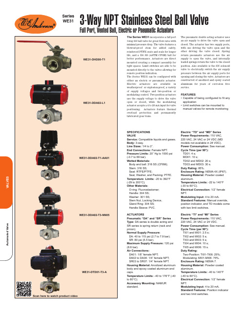
The Series WE31incorporates a full port 3-way SS ball valve for great flow rates with minimal pressure drop. The valve features a blowout-proof stem for added safety,reinforced PTFE seats and seals for longer life, and a 316 SS (ASTM CF8M) ball for better performance. Actuators are direct mounted creating a compact assembly for tight spaces. Limit switches are able to be mounted directly to the valves allowing for remote position indication.The Series WE31 can be configured with either an electric or pneumatic actuator.Electric actuators are available in weatherproof or explosion-proof, a variety of supply voltages and two-position or modulating control. Two-position actuators use the supply voltage to drive the valve open or closed, while the modulating actuator accepts a 4 to 20 mA input for valve positioning. Actuators feature thermal overload protection and permanently lubricated gear train.The pneumatic double acting actuator uses an air supply to drive the valve open and closed. The actuator has two supply ports,with one driving the valve open and the other driving the valve closed. Spring return pneumatic actuators use the air supply to open the valve, and internally loaded springs return the valve to the closed position. Also available is the SN solenoid valve to electrically switch the air supply pressure between the air supply ports for opening and closing the valve. Actuators are constructed of anodized and epoxy coated aluminum for years of corrosion free service.FEATURES•Capable of being configured to fit any application•Limit switches can be mounted to manual valves for remote monitoringSPECIFICATIONSVALVE Service:Compatible liquids and gases.Body: 3-way.Line Sizes:1/4 to 2˝.End Connections: Female NPT.Pressure Limits:20˝ Hg to 1000 psi(-0.7 to 69 bar).Wetted Materials:Body and ball: 316 SS (CF8M);Stem: 316 SS;Seat: RTFE/PTFE;Seal, Washer, and Packing: PTFE.Temperature Limits:-20 to 392°F(-29 to 200°C).Other Materials:O-ring: Fluoroelastomer;Handle: 304 SS;Washer: 301 SS;Stem Nut, Locking Device,Gland Ring: 304 SS;Handle Sleeve: PVC.ACTUATORSPneumatic “DA” and “SR” Series Type:DA series is double acting and SR series is spring return (rack and pinion).Normal Supply Pressure:DA: 40 to 115 psi (2.7 to 7.9 bar);SR: 80 psi (5.5 bar).Maximum Supply Pressure:120 psi (8.6 bar).Air Connections:DA01: 1/8˝ female NPT;DA02 to DA04: 1/4˝ female NPT;SR03 to SR07: 1/4˝ female NPT.Housing Material:Anodized aluminum body and epoxy coated aluminum end caps.Temperature Limits:-40 to 176°F (-40to 80°C).Accessory Mounting:NAMUR standard.Electric “TD” and “MD” Series Power Requirements: 110 VAC, 220 VAC, 24 VAC or 24 VDC (MD models not available in 24 VDC).Power Consumption:See manual.Cycle Time (per 90°): TD01: 4 s;MD01: 10 s; TD02 and MD02: 20 s; TD03 and MD03: 30 s. Duty Rating:85%.Enclosure Rating:NEMA 4X (IP67).Housing Material:Powder coated aluminum.Temperature Limits: -22 to 140°F (-30 to 60°C).Electrical Connection:1/2˝ female NPT.Modulating Input:4 to 20 mA.Standard Features:Manual override,position indicator, and TD models come with two limit switches. Electric “TI” and “MI” Series Power Requirements: 110 VAC, 220 VAC, 24 VAC or 24 VDC.Power Consumption:See manual.Cycle Time (per 90°):TI01 and MI01: 2.5 s; TI02 and MI02: 5 s;TI03 and MI03: 5 s; TI04 and MI04: 10 s;TI05 and MI06: 15 s.Duty Rating:Two-Position: TI01-TI06: 25%;Modulating: MI01-MI06: 75%.Enclosure Rating:NEMA 7.Housing Material:Powder coated aluminum.Temperature Limits:-40 to 140°F (-40 to 60°C).Electrical Connection:1/2˝ female NPT.Modulating Input:4 to 20 mA.Standard Features:Position indicator and two limit switches.3-Way NPT Stainless Steel Ball ValveFull Port, Vented Ball, Electric or Pneumatic ActuatorsSeries WE31Scan here to watch product videoFlow PathsACCESSORIESR2-2120,Air RegulatorAFR2-2, Instrument Air Filter Regulator VB-01, Volume Booster。
aoi的工作原理
aoi的工作原理AOI(Automated Optical Inspection)是一种自动光学检测技术,是通过使用光学系统和图像处理算法来检测电子产品制造过程中的缺陷和错误。
AOI工作原理是通过光学系统采集电子产品表面的图像,然后使用图像处理算法对图像进行分析和处理,最后根据事先设定的检测标准来判断产品的质量。
AOI系统需要采集电子产品表面的图像。
在生产过程中,电子产品经过各种工艺步骤,如焊接、贴片等,会形成各种不同的表面特征。
AOI系统通过使用高分辨率的摄像机和适当的光源来采集电子产品表面的图像。
光源的选择和光源的位置对于图像的质量和分析的准确性非常重要。
AOI系统使用图像处理算法对采集到的图像进行分析和处理。
图像处理算法主要包括图像增强、特征提取和缺陷检测等步骤。
在图像增强阶段,主要对图像进行降噪、增强对比度等处理,以提高图像质量。
在特征提取阶段,主要通过计算图像的特征参数,如边缘、纹理等,来描述电子产品表面的特征。
在缺陷检测阶段,主要通过比较采集到的图像与事先设定的标准图像或模板图像,来判断电子产品是否存在缺陷。
AOI系统根据事先设定的检测标准来判断产品的质量。
在生产过程中,制定了一系列的检测标准,如焊接质量、元器件位置等。
AOI系统通过与事先设定的标准进行比较,来判断电子产品是否符合要求。
如果检测到缺陷或错误,AOI系统会进行报警或标记,以便后续的处理和修复。
AOI工作原理的核心是光学系统和图像处理算法的配合。
光学系统负责采集图像,而图像处理算法则负责对图像进行分析和处理。
这种配合使得AOI系统能够快速、准确地检测电子产品的质量,提高生产效率和产品质量。
AOI工作原理是通过光学系统和图像处理算法对电子产品表面图像进行采集、分析和处理,最后根据事先设定的检测标准来判断产品的质量。
AOI系统的应用可以大大提高电子产品制造过程中的质量控制效率和准确性,为生产企业带来更大的经济效益。
ADAMS基础介绍

坐标系
状态栏
1.环境介绍
当前坐标值
7
机械系统动力学分析软件
ADAMS/View 工具栏浏览
12 34 56 78
1 几何建模
2 测量
4 铰接
3 恢复/重做
8力
5 色盘
9 10 11 12 13 14 15 16
6 运动驱动
7 移动
9 动态浏览 10 动态浏览 11 前后视图 12 左右视图
13 上下视图 14 背景视图 15 其它 16 视窗布置
模块)
Mechanism/Pro(Pro/Engineer
A/Flex(柔体分析模块)
接口模块)
A/Linear(系统模态分析模块)
CAT/ADAMS(与 CATIA 组合使用
A/Insight (统计分析模块)
的界面)
A/Hydraulics(液压模块)
工具箱模块
A/Vibration(振动分析)
• 自定义对话框
• 敏感度研究 •实验设计
ADAMS软件核心模块
1.环境介绍
6
机械系统动力学分析软件
ADAMS/View 窗口介绍
ADAMS/View…
主菜单 建模与仿真 工具面板 鼠标右键弹 出其它工具
模型标题
工作网格
控制面板
由上面的点 击命令出现 相应的控制 面板
下拉菜单
ADAMS软件核心模块
edges, or face normals Locations of existing
CSs or vertices
ADAMS软件核心模块
1.环境介绍
工作网格的显 示状态
9
机械系统动力学分析软件
Automated essay evaluation The Criterion online writing service

Grammar, Usage and Mechanics
The writing analysis tools identify five main types of errors—agreement errors, verb formation errors, wrong word use, missing punctuation, and typographical/proofreading errors. Some examples are shown in table 1. The approach to detecting violations of general English grammar is corpus-based and statistical. The system is trained on a large corpus of edited text, from which it extracts and counts sequences of adjacent word and part-of-speech pairs called bigrams. The system then searches student essays for bigrams that occur much less often than is expected based on the corpus frequencies. The expected frequencies come from a model of English that is based on 30-million words of newspaper text. Every word in the corpus is
scoring and evaluation. Work in automated essay scoring began in the early 1960s and has been extremely productive (Page 1966; Burstein et al. 1998; Foltz, Kintsch, and Landauer 1998; Larkey 1998; Rudner 2002; Elliott 2003). Detailed descriptions of most of these systems appear in Shermis and Burstein (2003). Pioneering work in the related area of automated feedback was initiated in the 1980s with the Writer’s Workbench (MacDonald et al. 1982). The Criterion Online Essay Evaluation Service combines automated essay scoring and diagnostic feedback. The feedback is specific to the student’s essay and is based on the kinds of evaluations that teachers typically provide when grading a student’s writing. Criterion is intended to be an aid, not a replacement, for classroom instruction. Its purpose is to ease the instructor’s load, thereby enabling the instructor to give students more practice writing essays. Criterion contains two complementary applications that are based on natural language processing (NLP) methods. Critique is an application that is comprised of a suite of programs that evaluate and provide feedback for errors in grammar, usage, and mechanics, that identify the essay’s discourse structure, and that recognize potentially undesirable stylistic features. The companion scoring application, e-rater version 2.0, extracts linguistically-based features from an essay and uses a statistical model of how these features are related to overall writing quality to assign a holistic score to the essay. Figure 1 shows Criterion’s interface for submit-
机械制造专业英语专有名词缩写
机械制造专业英语缩写AC=alternative current交流AGV=Automated Guided Vehicle自动导引小车AGVS= Automated Guided Vehicle System自动导引小车系统AMT=advanced manufacturing technology先进制造技术ANSI=American National Standards Institute美国国家标准协会APT=Automatically Programmed Tools自动数控程序BOM=Bill of Material物料清单CAA=Computer Aided Analysis Process计算机辅助分析过程CAD=Computer-Aided Design计算机辅助设计CADD=Computer-Aided Design Drafting计算机辅助设计制图CAE=computer aided engineering计算机辅助工程CAM=Computer-Aided Manufacturing计算机辅助制造CAIT=computer aided testing and inspection计算机辅助实验与检测CAPP=Computer Aided Process Planning计算机辅助工艺设计CHP=chemical Polishing 化学抛光CIM=Computer integrated manufacturing计算机集成制造CBN=Cubic Boron Nitride立方氮化硼CMM=Coordinate Measuring Machine三坐标测量机CNC=computer numerical control电脑数字控制DC=direct current直流DNC=Direct Numerical Control直接数字控制DOF=degrees of freedom自由度DXF=data exchange format数据交换格式ECM=Electrochemical Machining电解加工EBM=Electron beam machining电子束加工EDM=Electrical Discharge Machining电火花加工EGM= enhanced graphics module增强型图形模组FA=factory automation工厂自动化FDM=Fused Deposition Modelling熔融沉积成型FEA=Finite element analysis有限元分析FMC=flexible manufacturing component柔性制造单元FMS=Flexible Manufacturing System柔性制造系统Finite-element有限元Four-bar linkage四连杆机构GNC=graphical numerical control图形数控GT=Grease Trap润滑脂分离器HPM=hard-part machining硬态切削HSS=High-Speed-Steel高速钢IGES=initial graphic exchange specification初始图形交换规则ISO=International Standardization Organization国际标准组织IT=International Tolerance(grade)国际公差JIT=Just in Time准时生产LBM=Laser beam machining激光切削加工LED=light-emitting diode发光二级管LMC=least material condition最小实体状态LOM=Laminated Object Manufacturing叠层实体制造技术MMC=maximum material condition最大实体状态MATL=material材料MC=machining center加工中心NC=Numerical Control数字控制NMP=Nontraditional Manufacturing Processes特种加工技术PCB=printed circuit boards印刷电路板PLC=Programmable Logic Controller PLC控制PKW=parallel kinematics machine并联机床QTY=quantity required需求数量RGV=rail guided vehicle有轨自动导引小车RPM=Rapid Prototype Manufacturing快速成型技术SL= Stereo Lithography光固化成型SLA=Stereo Lithography Apparatus立体印刷技术/光固化立体造型SLS=Selective Laser Sintering选择性激光烧结USM=Ultrasonic Machining超声波加工VNC=voice numerical control声音控制WEDM=Wirecut Electrical Discharge Machining电火花线切割加工WJM/C=water-jet machining/cutting水射流切削3D PRINT 3D打印。
- 1、下载文档前请自行甄别文档内容的完整性,平台不提供额外的编辑、内容补充、找答案等附加服务。
- 2、"仅部分预览"的文档,不可在线预览部分如存在完整性等问题,可反馈申请退款(可完整预览的文档不适用该条件!)。
- 3、如文档侵犯您的权益,请联系客服反馈,我们会尽快为您处理(人工客服工作时间:9:00-18:30)。
Automated estimation and analyses of meteorological drought characteristics from monthly rainfall dataV.U. Smakhtin and D.A. HughesAbstractThe paper describes a new software package for automated estimation, display and analyses of various drought indices – continuous functions of precipitation that allow quantitative assessment of meteorological drought events to be made. The software at present allows up to five different drought indices to be estimated. They include the Decile Index (DI), the Effective Drought Index (EDI), the Standardized Precipitation Index (SPI) and deviations from the long-term mean and median value. Each index can be estimated from point and spatially averaged rainfall data and a number of options are provided for months' selection and the type of the analysis, including a running mean, single value or multiple annual values. The software also allows spell/run analysis to be performed and maps of a specific index to be constructed. The software forms part of the comprehensive computer package, developed earlier and designed to perform the multitude of water resources analyses and hydro-meteorological data processing. The 7-step procedure of setting up and running a typical drought assessment application is described in detail. The examples of applications are given primarily in the specific context of South Asia where the software has been used.Software availabilityPackage:The SPATSIM software package;Availability:From the Institute for Water Research (IWR) at Rhodes University;Cost:No development cost involved, the Institute is obliged to pass on the application development licensecosts charged by ESRI. This amounts to approximately 200 USD;Description:Available on IWR website http://www.ru.ac.za/institutes/iwr/. Updates to the software are regularlyposted on the IWR website and readily downloaded at no cost by registered users1. IntroductionMeteorological droughts are temporary, recurring natural disasters, which originate from the lack of precipitation and can bring significant economic losses. It is not possible to avoid meteorological droughts, but they can be predicted and monitored, and their adverse impacts can be alleviated. The success of the above depends, amongst the others, on how well the droughts are defined and drought characteristics quantified. Quantitative drought definitions identify the beginning, end, spatial extent and severity of a drought. They are often region-specific and are based on scientific reasoning, which follows the analysis of certain amounts of hydro-meteorological information. Quantitative definitions of a drought are formulated in terms of drought indices.Drought indices are normally continuous functions of rainfall and/or temperature, river discharge or other measurable hydrometeorological variable. A large number of drought indices have been suggested to date, including Palmer Drought Severity Index (PDSI – Palmer, 1965), Crop Moisture Index (CMI – Palmer, 1968), Standardized Precipitation Index (SPI – McKee et al., 1993), “Deciles” (Gibbs and Maher, 1967), FAO water satisfaction index (Frere and Popov, 1979), Agro-hydro Potential (AHP – Petrasovits, 1990), Index of Moisture Adequacy (IMA – Sastri, 1993), Surface Water Supply Index (SWSI – Shafer and Dezman, 1982), and multiple indices of low river flow (Smakhtin, 2001). Some of these indices focus on the degree to which crop moisture requirements are met (e.g. CMI, AHP, IMA above), others intend to assess the lack of overall water availability in a region or a river basin (SWSI above). Yet others are flexible enough to identify, assess and monitor drought progress over the range of temporal scales and therefore evaluate different types of water shortages (SPI above).Reviews of drought indices may be found in many sources, including(/whatis/indices.htm, Tate et al., 2000 and Smakhtin and Hughes, 2004).The inherent complexity of drought phenomena implies that no drought index is ideal for all regions or tasks. In most cases, it is useful and necessary to consider more than one index, examine the sensitivity and accuracy of indices, the correlation between them and explore how well they compliment each other in the context of a specific research or management objective (Guttman, 1998, Wu et al., 2001 and Morid et al., 2006). Many computer programs and on-line tools were developed to estimate either individual indices separately, or several indices at once (e.g. Wu et al., 2001 and Rossi and Cancelliere, 2003;/whatis/indices.htm; National Agricultural Decision Support System (NADSS) ). Consequently, the need to simply calculate various drought indices is not, on its own, sufficient justification for a new software development. It is, however, important to ensure that drought is seen as a comprehensive water resources issue and is assessed within a comprehensive water resources software environment. Facilities should exist to import information from multiple raw data formats, display and analyze various drought indices in a variety of ways, convert point rainfalls and drought indices to representative areal values, perform rapid spatial analysis of different drought characteristics and link to various hydrological, ecological and water resources models to analyze different components of droughts and to interpret their outputs. The automation of these procedures could facilitate data intensive, regional drought analyses (e.g. Lloyd-Hughes and Saunders, 2002).Considering the number and magnitude of the requirements listed above, it is logical to consider incorporating drought estimation and analyses routines into an existing software package, which already has some of the required features, is flexible enough to work efficiently with large data sets, is cost effective and is continuously developing to include more components relevant to drought analyses. This paper describes the incorporation of several drought assessment modules into one such package designed to cover a much wider range of water resources applications. The paper describes the general features of this package followed by a description of several selected drought indices and the steps necessary to set up, run and examine the results of a typical drought analysis application.2. General features of the SPATSIM software packageThe SPATSIM (SP atial and T ime S eries I nformation M odeling) software package has been under development at the Institute for Water Research (IWR) of Rhodes University, South Africa since 1999 (Hughes and Forsyth, in press). It is a relatively new software product which is quickly gaining recognition in South Africa and other countries. It has been applied extensively in southern Africa (South Africa, Zimbabwe, Zambia, Tanzania, Swaziland and Angola) for various water resource analysis studies including environmental flow assessments and hydrological model based water resource determinations.The package has been developed in Delphi using ESRI Map Objects as a tool for managing and modeling the data that are typically associated with water resource assessment studies. It contains an integrated database management system that uses GIS shape files as the main form of data access. It has a number of built-in data analysis and processing tools, such as for generating catchment average rainfall data from gauged station data or generating monthly and annual frequency tables from time series data. It also includes a wide range of external models that can be setup and integrated seamlessly with the database, i.e. the models access their data requirements from the SPATSIM database and store their results in the database without any intermediate data transformation. The models include spatial interpolation of observed flow records (Hughes and Smakhtin, 1996), monthly rainfall–runoff simulation (Hughes, 2004) and a desktop model for environmental flow assessment (Hughes and Münster, 2000). SPATSIM has a comprehensive set of Help facilities, and all new users can consult ‘Help’ to obtain a basic understanding of the system and how to make use of the various menu items. A detailed description of SPATSIM can be found on the IWR website (http://www.ru.ac.za/institutes/iwr – see the link to Hydrological Models and Software), as well as in Hughes and Forsyth (in press).SPATSIM's flexible environment provided an excellent opportunity to incorporate drought assessment or management routines. Considering that such analyses are carried out by many centres and individuals throughout the world, the drought assessment routines should:• ensure that existing data import facilities are satisfactory for a variety of drought assessment projects (and associated data formats) and cater for the requirements of various future users;• have facilities for generating time series of drought indices from station rainfall data and from areal rainfall data interpolated from station (i.e. point) rainfall data;• provide a range of facilities for further display and regional analysis of drought indices;• provide clear in-built documentation of all drought indices and drought–related facilities in the SPATSIM‘Help’ system.3. Drought indices currently included in SPATSIMThe software package currently includes five drought indices: the Standardized Precipitation Index (SPI), the Decile Index (DI, or “deciles”), the Effective Drought Index (EDI) and the departures from the long-term mean and median precipitation values. The commonality between all these indices is that they are calculated exclusively on the basis of monthly rainfall data. Rainfall data are widely used to calculate drought indices, because long-term rainfall records are more readily available than other types of hydrological or climatic data. While rainfall data alone may not reflect the spectrum of drought related conditions, they can serve as a pragmatic solution in data-poor regions and as a useful point of departure in drought software development. Although the indices are normally referred to here and elsewhere as “drought indices”, all of them can effectively be used for the assessment of both dry and wet conditions. A brief description of the indices and their implementation in SPATSIM is given below. A potential user of the system, however, is advised to consult the original literature sources, explaining each and every drought index in more detail. This is a necessary pre-requisite for understanding the advantages and limitations of the indices, as well as of the modifications to the original algorithms, which have been introduced in SPATSIM3.1. Standardized Precipitation Index (SPI)The SPI index was developed by McKee et al. (1993). In its original version, a long-term precipitation record at a station is fitted to a probability (gamma) distribution, which is then transformed into a normal distribution so that the mean SPI is zero. The index values are therefore the standardized deviations of the transformed rainfall totals from the mean. The SPI may be computed with different time steps (1 month, 3 months, 24 months, etc.) to facilitate the assessment of the effects of a precipitation deficit on different water resources components (groundwater, reservoir storage, soil moisture, streamflow). Positive SPI values indicate greater than median precipitation and negative values indicate less than median precipitation. Drought periods are represented by relatively high negative deviations. Normally, the “drought” part of the SPI range is arbitrary split into moderately dry (−1.0 > SPI > −1.49), severely dry (−1.5 > SPI > −1.99) and extremely dry conditions (SPI < −2.0). A drought event starts when SPI value reaches −1.0 and ends when SPI becomes positive again (McKee et al., 1993). In the SPATSIM application, there are several options available for accumulating the monthly rainfall values into a time series before the SPI (or any other index) is calculated. These options are explained latter in the text. The time series is then normalized using an automated procedure to optimize the λ (lambda) parameter of the Box–Cox approximation for transformation to a normal distribution, using equations:(1)where x is the original variable (rainfall) and y is the transformed variable.3.2. DecilesIn this method, originally suggested by Gibbs and Maher (1967), monthly precipitation totals from a long-term record are first ranked from highest to lowest to construct a cumulative frequency distribution. The distribution is then split into 10 parts (deciles). The first decile is the precipitation value not exceeded by the lowest 10% of all precipitation values in a record, the second is between the lowest 10 and 20%, etc. Any precipitation value (e.g.from the current or past month) can be compared with and interpreted in terms of these deciles. Decile Indices (DI) are often grouped into five classes, two deciles per class. If precipitation falls into the lowest 20% (deciles 1 and 2), it is classified as “much below normal”. Deciles 3 and 4 (20–40%) indicate “below normal” precipitation, deciles 5 and 6 (40–60%) give “near normal” precipitation, deciles 7 and 8 (60–80%) “above normal” and deciles 9 and 10 (80–100%) are “much above normal”.The original DIs are therefore integer numbers (1–5 or 1–10), while in SPATSIM, no attempt is made to convert the actual frequency (exceedence) values into DI groups. The time series of this drought index is therefore based on the same type of analysis as the original decile of Gibbs and Maher (1967), but is represented by actual frequency values in percent instead of decile integer numbers.3.3. Effective Drought Index (EDI)Unlike many other drought indices, the EDI in its original form (Byun and Wilhite, 1996) is calculated with a daily time step. However, its principles can be used similarly with monthly precipitation data as is done in SPATSIM and described below. The EDI is a function of precipitation needed for a return to normal conditions (PRN). PRN is precipitation, which is necessary for the recovery from the accumulated deficit since the beginning of a drought. PRN, in turn, effectively stems from monthly effective precipitation (EP) and its deviation from the mean for each month.The first step is the calculation of EP, defined as a function of the current month's rainfall and weighted rainfall over a defined preceding period (selected by the duration option in SPATSIM, see below). If P m is the rainfall m-1 months before the current month and N is the duration of preceding period then the EP for the current month is:(2)For example, if N = 3 then EP = P1 + (P1 + P2)/2 + (P1 + P2 + P3)/3, where P1, P2 and P3 are precipitation values during the current month, previous month and 2 months before, respectively. The mean and standard deviations of the EP values for each month are then calculated and the time series of EP values is converted to deviations from the mean (DEP). PRN values are then calculated as:PRN=DEP/∑(1/N) (3)The summation term is the sum of the reciprocals of all the months in the duration N (i.e. for N = 3 months, this term will be equal to: 1/1 + 1/2 + 1/3). Finally the EDI is calculated as:EDI=PRN/Std(PRN) (4)where Std (PRN) is the standard deviation of the relevant month's PRN values. In this algorithm, no normalization of the index or rainfall data is performed and therefore the skewness of the original time series is preserved. This means that positively skewed rainfall data can result in a larger range of positive EDI values than the range of negative EDI values. This is not, however, seen as a critical issue as the negative values are the important ones in that they represent the ‘rainfall’ that is required for a return to normal from a drought.Similar to the SPI, the EDI values are standardized, which allows drought severity at two or more locations to be compared with each other regardless of climatic differences between them. The EDI also has thresholds indicating the range of wetness – from extremely dry to extremely wet conditions. The “drought range” of the EDI indicates extremely dry conditions at EDI < −2, severe drought at −1.5 > EDI> −1.99 and moderate drought at−1.0 > EDI > −1.49. Near normal conditions are indicated by−0.99 < EDI < 0.99.3.4. Departure from the mean and medianThese indices are simple by definition, easy to calculate and are easily understood by a general audience. They are also the variations of the “percent of normal”. “Normal” may be and usually is set to a long-term mean or medianprecipitation value. For example, meteorological drought in India is defined when rainfall in a month or a season is less than 75% of its long-term mean. If the rainfall is 50–74% of the mean, a moderate drought event is assumed to occur, and severe drought occurs when rainfall is less than 50% of its mean (e.g. Khan, 1998). Droughts in South Africa are defined as periods with less than 70% of normal precipitation. This becomes a severe drought when two consecutive seasons experience 70% of normal rainfall or less (Bruwer, 1990). There are many other similar indices and associated drought definitions (Tate et al., 2000). They are normally region-specific and explicitly set locally appropriate rainfall limits and durations of rainless periods for the definition of droughts of different extremes. In SPATSIM, the Departure from the Mean and Departure from the Median are simple measures of rainfall deviation (from mean or median for the selected period, respectively) and are neither normalized nor standardized.4. Setting up a typical drought assessment application4.1. Step 1: Organize SPATSIM features (spatial coverages)SPATSIM uses spatial features (coverages) and temporal attributes (time series, Fig. 1). The assumption is that there will be at least two available coverages: one point coverage representing raingauge locations for raw monthly rainfall data and one polygon coverage representing administrative areas or catchments. If the latter is not available, the facility in SPATSIM can be used to establish a new polygon coverage of equal size grid squares. This can then be used to generate the areal rainfall data from the point rainfall and to display the spatial variation of drought indicesFig. 1. The main SPATSIM screen, showing part of South Asia region, with the selection windows for available spatial features and attributes, associated with the highlighted feature.4.2. Step 2: Create main SPATSIM attributes (time series)It is necessary to design the SPATSIM attribute structure to store and manage the raw and processed data. This simply involves adding new attributes of different types and giving them suitable names that can be recognized later. For the raingauge point coverage, the minimum requirement will be a time series attribute that will be used to store the raw monthly rainfall data. For the polygon coverage that will be used for generating the spatially distributed drought indices, a wide range of attributes may be required depending on the analyses intended. At least a time series attribute will be needed that will be used to store the area average rainfall data interpolated from the point rainfall data.Additional time series attributes will be required for each drought index that is to be generated and it is important to name these carefully so that they can be readily identified for future analysis purposes. Fig. 2 indicates that there is a wide variety of index values that can be generated (see step 5 for more details). Users could get confused trying to remember which drought index has been stored in which attribute. That is why it is essential to use recognizable names for the attributes. For example ‘SPI Annual 3m Jan’ could be used for an SPI based on a single annual value with a 3-month duration starting in January. ‘SPI 12m RunM’ might be used for an SPI value based on 12-month running means. The lower right hand box displays all the available attributes that have been established in an example application (Fig. 2). SPATSIM has a facility (the memo attributes), which can be used to provide a key to the information stored within other attributes.Fig. 2. Main drought index generation screen showing the various drought index options that are available, help window and example time series calculated (right window).4.3. Step 3: Import raw rainfall dataA set of time series data import routines are available to load suitably formatted text files of monthly rainfall data to the SPATSIM time series attribute associated with the point raingauge feature. There are a wide variety of options available to ensure that various original formats can be imported. One common format is the‘spreadsheet’ type: annual plus 12 monthly values per line in a text file with a defined number of explanation lines above the data – called the header. Another common format is the ‘continuous data’ type (the start date – e.g. day/month/year – followed by one data value per line). Common problems are related to the lack of line feeds and carriage return codes at the end of the text lines when exported from other specialist software. These can usually be solved by importing the data into a text editor and then simply saving the data. Bulk data imports can be achieved by naming the raw data text files with the same text as the spatial element (points) labels.4.4. Step 4: Generate areal rainfall dataA procedure is provided to generate areal rainfall data for a polygon feature from point rainfall data. It uses the inverse distance squared interpolation method and data sets from rainfall stations located within a user-defined search radius. The procedure fills missing data and generates complete records for all the polygons to be used. The examples of polygons include catchments, administrative divisions or a rectangular grid. If the procedure cannot find a rainfall value for a particular month at any station within a defined search radius, mean monthly rainfall values for identified stations are used to calculate a polygon rainfall value for this month. This can be a problem if there are extended missing data periods within several raingauge time series in the same area. However, the problem is usually quite easy to recognize as a repeating pattern of rainfall will be seen in the areal rainfall time series viewed using the SPATSIM display facilities (see step 7). The user can visually compare and inspect the data series to ensure that the areal interpolation process has worked successfully. Other problems that can occur are related to an inappropriate search radius, insufficient raingauges in a particular area, or selection of too few (or too many) raingauges on which to base the interpolation.4.5. Step 5: Generate drought indicesThis procedure is used to generate time series of a range of drought indices from complete (no missing data) time series of monthly rainfall. The input data for the analysis will be the data associated with the currently selected attribute (a time series of rainfall) and feature.A user can select from various options for different index types and ensure that the destination attribute selected for storing the data has an appropriate name to identify what data are being stored (see step 2). The user has the flexibility of choosing different durations, starting months and data integration types (Fig. 2). The analysis options and duration selections are disabled if they are not appropriate to a specific index that has been selected. Most indices can be calculated as multiple annual values, single annual value or running mean values. This step can be repeated for as many different index types as required.The first option (multiple annual values) allows the starting month and durations of 1,2,3,4 or 6 to be selected. If January and 3 months duration is selected, the groups of months which will be analyzed are JFM, AMJ, JAS, OND (the capital letters here stand for the month: J – for January, F – for February, etc).The second option (single annual value) allows the starting month and durations of 1–12 to be selected. In all cases, only 1 value per year is generated based on rainfall accumulated over the duration from the start month. For example, if January and 6 months are selected, the annual values will be based on rainfall accumulated for JFMAMJ (January–June), while the rainfall for the other months will be ignored.The third option (running mean/total values) is similar to the first (multiple annual values), but 12 values per year are always generated regardless of the selected duration. The selected duration can be any value up to 48 months. If a duration of 6 months is selected and the rainfall data start in January 1960, the first index value will be based on rainfall accumulated for 1960 JFMAMJ, the second for 1960 FMAMJJ, the third for 1960 MAMJJA, etc. This procedure is similar to the original SPI calculation proposed by McKee et al. (1993).4.6. Step 6: Generate summary drought index informationGenerating summary information on drought indices is necessary if subsequent mapping of index values is required (step 7). Two types of drought index summary information can be generated, both at the same time (Fig.3). The first option is a summary of actual index values. The second option is a summary of the run (or spell) characteristics of the index data (i.e. for how long a drought index continuously lies below and above a certain critical threshold).Fig. 3. A screen for saving drought index information to a summary table.In both cases data are extracted for up to 10 sample years from a time series of drought index values and stored in a 2-D array type attribute (year, polygon). The summary data for many different drought indices could be stored and therefore the naming approach for the attributes within SPATSIM is very important. The choice of storing a sample of 10 values is quite arbitrary, but is based on the assumption that a larger number would be rather unnecessary and, if required, could be stored within more than one summary attribute. In certain cases (i.e. where there are multiple drought index values per year), it is necessary to select not only the years but also the month for the required drought index. While multiple years can be selected, multiple months cannot to avoid confusion (i.e.a user may select several years for the period JAS, but cannot select JFM, AMJ, JAS and OND for 1968). The same set of years but with a different month group may, however, be selected and stored.The analysis is based on the time series attribute that is current at the time of running the procedure. This process can therefore be repeated as many times as necessary to store summary data for all the drought indices generated during step 5.4.7. Step 7: Displaying drought index informationTwo groups of display facilities are available in SPATSIM to visualize drought index information (or any water resources information and data). The first allows the generated time series of any drought index (step 5) to be displayed. The second allows polygon features to be classified and mapped using generated index summary information (step 6).Drought index time series can be displayed and compared using the SPATSIM display facility (TSOFT) for a range of polygons (or different index types for the same polygon). In other words, it is possible to compare the same index for several areas, or display different index time series for the same area (Fig. 4). Within TSOFT, additional analysis facilities are available to assess the frequency or run/spell characteristics of the drought indices. The ‘Help’ system provides information about how to load time series data into TSOFT.Fig. 4. Example screen showing graphs of areal monthly rainfall (top plot) and time series of 3 months' running SPI and EDI values (bottom plot). Both examples are for arbitrary selected polygon – a district in Rajasthan state of India. The legend for each plot, color schemes, scaling options and additional analysis with the displayed time series are available through various options under “Graph”, “Display” and “Analysis” menu items.Drought summary information allows the areal extent and pattern of droughts for a specific year (or season of a year) to be examined using either actual indices extracted or run/spell characteristics. In both cases, it will be necessary to select the summary information required from one of the stored array attributes and to specify the ranges and colors of the drought index categories to be used for classifying the polygons. For the SPI index it has been found useful to set the minimum value to –2.5, the interval to 0.5 and the number of groups to 9. When mapping the DI (deciles) values based on the frequency data, it is suggested that five groups are used with a minimum value of 0 and an interval of 20. However, users have full flexibility in defining drought categories in any way desired.The final result is a map of color coded index values for those polygons that have data associated with them (Fig.5). To start another mapping with a different index, the existing one must be removed. A legend is not drawn on the Map as facilities to do this neatly are not available within the Map Objects development software. It is possible that a better way of doing this will be found in the future.。