LQG predictive optimal control for adaptive applications

合集下载

电气工程与自动化专业英语(李军)第13章

It is worth pointing out that there are no hard-lines limits among the classification and the resulting controllers above. Here we present a personal overview on Advanced Control Methods as follows: Adaptive Control: 1. Be defined as a feedback control system intelligent enough to adjust its characteristics in a changing environment. 1. Traditional adaptive control methods, either model reference or self-tuning, usually require some kind of
Add Your Company Slogan
Chapter 13: Adaptive Control and Predictive Control
Adaptive Control and Predictive Control
Before introduction to the advanced control design techniques, we present a brief overview of control techniques and paradigms： The 1950s gave rise to the state-space formulation of differential equations The method of dynamic programming was developed by Bellman (1957) The maximum principle was discussed by Pontryagin (1962).

博士生研究发现新型神经退行性疾病的治疗靶点

博士生研究发现新型神经退行性疾病的治疗靶点神经退行性疾病是一类常见且严重的神经系统疾病，如阿尔茨海默病、帕金森病和亨廷顿病等。

这些疾病的特点是神经细胞的异常死亡和功能丧失，导致相关脑区和神经递质的改变。

然而，目前对于这些疾病的治疗选项非常有限。

近期的一项研究取得突破性进展，博士生研究人员发现了新型神经退行性疾病的治疗靶点，为未来的治疗提供了新的希望。

该研究由博士生李明领导的团队进行，他们针对神经退行性疾病的发病机制进行了深入研究。

通过使用先进的基因编辑技术和转基因小鼠模型，研究人员发现了一种新型的蛋白质复合物，命名为RDF （Regulator of Degenerative Factors）。

RDF在神经退行性疾病的病理过程中发挥着重要的调控作用。

研究结果显示，RDF复合物具有调控炎症反应和神经细胞死亡的功能。

在神经退行性疾病模型中，RDF的表达水平显著下降。

通过增加RDF的表达，研究人员观察到神经细胞的存活率得到显著提高，并且炎症反应得到抑制。

此外，进一步的实验发现，RDF可以与特定的信号通路分子相互作用，从而进一步调节神经细胞的存活和功能。

基于这些发现，研究人员开始寻找RDF的调控机制。

他们发现一种名为NF-κB（核因子κB）的转录因子可以结合到RDF上，从而增加其表达。

NF-κB是炎症反应的重要调控分子，与神经退行性疾病的发病机制密切相关。

通过调控NF-κB信号通路，研究人员能够有效地改变RDF的表达水平，从而对神经细胞起到保护作用。

这项研究的发现为新型神经退行性疾病的治疗提供了新的方向。

研究人员认为，通过调节RDF和NF-κB信号通路，可以改变神经退行性疾病的发病过程，从而减轻病情并延缓疾病的进展。

此外，研究人员还证实了一种名为RDF增效剂的分子，可以增加RDF的稳定性和活性，进一步提高治疗效果。

然而，尽管这一研究取得了重要的突破，但仍有许多工作需要进行。

首先，研究人员需要进一步探索RDF的分子机制，以更好地理解其在神经退行性疾病发病过程中的作用。

基于LQG控制的EPS系统最优控制研究

技术创新控制系统您的论文得到两院院士关注基于LQG 控制的EPS 系统最优控制研究Optimal control Research for Electric Power Steering System Based on LQG Controller(山东理工大学)高士香石沛林邹广德苗立东GAO Shi-xiang SHI Pei-lin ZOU Guang-de MIAO Li-dong摘要:电动助力转向系统存在着路面随机激励、转矩传感器测量噪声、模型参数不确定所引起的干扰等复杂因素,通过建立电动助力转向系统的数学模型以及加入随机干扰信号的系统状态空间表达式,设计了线性二次型高斯状态反馈控制器和Kalman 滤波器。

并以能耗及电机的实际助力电流与目标助力电流之间的误差最小为目标函数对EPS 系统进行仿真分析,仿真结果表明:采用该最优控制方法能有效的抑制系统的外部干扰,提高系统的鲁棒性,使能耗及电机的实际助力电流与目标助力电流之间的误差达到最小。

关键词:电动助力转向系统;LQG 控制器;卡尔曼滤波;最优控制中图分类号:U463.4文献标识码:A Abstract:Because of the complex factors of the random road excitation,the measurement noises of the torque sensor and the distur -bance of model errors in the electric power steering system,the mathematical models of electric power steering system were estab -lished and the state -space formula with random disturbance signal was performed.Then the LQG state feedback controller and theKalman filter were designed.Finally,take minimum the energy consumption and the error between the actual current of assist motor and the target value as the target function and simulate.The simulation results showed that this optimal control method could attenu -ate the external disturbance effectively,improve the system robustness,and minimize the energy consumption and the error between the actual assist current of motor and the target current.Key words:electric power steering system;LQG controller;Kalman filter;optimal control文章编号:1008-0570(2010)03-1-0071-021引言电动助力转向系统采用电机直接提供转向助力来帮助驾驶员转向,从而减轻驾驶员的操纵力,提高汽车操纵的轻便性和灵活性。

《2024年基于机器学习算法的超材料快速自动设计研究》范文

《基于机器学习算法的超材料快速自动设计研究》篇一一、引言超材料作为一种具有独特物理特性的新型材料，近年来在众多领域中得到了广泛的应用。

然而，超材料的设计往往需要复杂的物理模型和精细的实验验证，导致设计过程既耗时又昂贵。

因此，寻求一种高效、自动化的超材料设计方法成为了科研领域的迫切需求。

本文提出了一种基于机器学习算法的超材料快速自动设计方法，旨在通过算法的智能优化来提高超材料设计的效率和准确性。

二、研究背景及意义随着人工智能和机器学习技术的快速发展，其在材料科学领域的应用也越来越广泛。

通过机器学习算法，我们可以从大量的材料数据中学习并发现材料性质与结构之间的内在规律，为材料的快速设计和优化提供有力支持。

将机器学习算法应用于超材料设计，不仅可以提高设计效率，还可以降低实验成本，推动超材料在各个领域的应用。

三、研究方法本研究采用了一种基于深度学习的机器学习算法，通过构建超材料设计的智能优化模型，实现超材料的快速自动设计。

具体步骤如下：1. 数据准备：收集超材料的相关数据，包括材料的组成、结构、性质等，建立超材料数据库。

2. 特征提取：从超材料数据库中提取对设计有用的特征，如材料的组成比例、结构参数等。

3. 构建模型：利用深度学习算法，构建超材料设计的智能优化模型。

该模型可以根据提取的特征，预测材料的性质和性能。

4. 模型训练与验证：使用部分数据对模型进行训练和验证，确保模型的准确性和可靠性。

5. 自动设计：将模型应用于超材料的自动设计过程中，根据设计要求，自动寻找满足条件的材料组成和结构。

四、实验结果与分析通过实验，我们验证了基于机器学习算法的超材料快速自动设计方法的有效性和准确性。

实验结果如下：1. 设计效率：与传统的超材料设计方法相比，基于机器学习算法的设计方法可以大大提高设计效率。

在同样的时间内，可以设计出更多的超材料方案。

2. 设计准确性：机器学习模型可以准确预测超材料的性质和性能，降低实验验证的次数和成本。

最优跟踪控制概念

最优跟踪控制概念全文共四篇示例，供读者参考第一篇示例：最优跟踪控制（Optimal Tracking Control）是自动控制领域中的一个重要概念，旨在设计控制系统使其能够通过自动调节来跟踪某个期望轨迹或信号，以实现系统的最佳性能。

在实际应用中，最优跟踪控制被广泛应用于各种领域，如航空航天、机器人技术、汽车控制等。

本文将探讨最优跟踪控制的基本概念、方法以及在实际应用中的重要性。

最优跟踪控制的基本概念是通过控制系统来实现对系统的期望轨迹或信号的跟踪。

在实际应用中，系统通常会受到各种干扰和噪声的影响，因此设计一个稳健的控制策略成为至关重要的任务。

最优跟踪控制方法通过最小化系统性能指标（如误差或能量）来实现系统的最佳控制性能，从而使系统能够快速、准确地跟踪期望轨迹或信号。

在最优跟踪控制方法中，一种常用的方法是使用最优控制理论。

最优控制理论是一种数学优化方法，通过对系统动力学方程进行最优控制设计，以最小化系统性能指标。

在最优跟踪控制中，通常会使用线性二次型最优控制（LQ控制）或线性二次型高斯最优控制（LQG控制）等方法来实现系统的最佳控制性能。

最优跟踪控制方法还可以结合模型预测控制（MPC）等方法来优化控制策略。

模型预测控制是一种基于模型的控制方法，通过对系统的模型进行预测来优化控制策略。

在最优跟踪控制中，可以使用模型预测控制来实现对系统的期望轨迹或信号的跟踪，从而提高系统的性能和稳定性。

在实际应用中，最优跟踪控制在各种领域都发挥着重要作用。

在航空航天领域，最优跟踪控制被广泛应用于飞行器的自动驾驶系统，以实现飞行器的姿态控制和航线跟踪。

在机器人技术领域，最优跟踪控制被用于设计机器人的运动控制系统，以实现机器人在复杂环境中的准确和稳定的运动。

在汽车控制领域，最优跟踪控制被用于设计车辆的自动驾驶系统，以实现车辆的路径规划和跟踪。

最优跟踪控制是自动控制领域中的一个重要概念，通过最优化控制策略来实现系统的最佳性能。

Introduction+to+Model+Predictive+Control

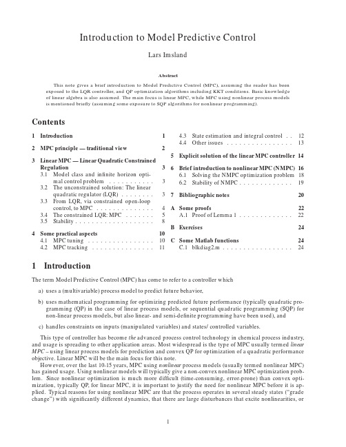
Introduction to Model Predictive ControlLars ImslandAbstractThis note gives a brief introduction to Model Predictive Control(MPC),assuming the reader has been exposed to the LQR controller,and QP optimization algorithms including KKT conditions.Basic knowledge of linear algebra is also assumed.The main focus is linear MPC,while MPC using nonlinear process models is mentioned brieﬂy(assuming some exposure to SQP algorithms for nonlinear programming). Contents1Introduction1 2MPC principle—traditional view2 3Linear MPC—Linear Quadratic Constrained Regulation33.1Model class and inﬁnite horizon opti-mal control problem (3)3.2The unconstrained solution:The linearquadratic regulator(LQR) (3)3.3From LQR,via constrained open-loopcontrol,to MPC (4)3.4The constrained LQR:MPC (5)3.5Stability (8)4Some practical aspects104.1MPC tuning (10)4.2MPC tracking (11)4.3State estimation and integral control..124.4Other issues (13)5Explicit solution of the linear MPC controller14 6Brief introduction to nonlinear MPC(NMPC)166.1Solving the NMPC optimization problem186.2Stability of NMPC (19)7Bibliographic notes20 A Some proofs22A.1Proof of Lemma1 (22)B Exercises24C Some Matlab functions24C.1blkdiag2.m (24)1IntroductionThe term Model Predictive Control(MPC)has come to refer to a controller whicha)uses a(multivariable)process model to predict future behavior,b)uses mathematical programming for optimizing predicted future performance(typically quadratic pro-gramming(QP)in the case of linear process models,or sequential quadratic programming(SQP)for non-linear process models,but also linear-and semi-deﬁnite programming have been used),andc)handles constraints on inputs(manipulated variables)and states/controlled variables.This type of controller has become the advanced process control technology in chemical process industry, and usage is spreading to other application areas.Most widespread is the type of MPC usually termed linear MPC–using linear process models for prediction and convex QP for optimization of a quadratic performance objective.Linear MPC will be the main focus for this note.However,over the last10-15years,MPC using nonlinear process models(usually termed nonlinear MPC) has gained ing nonlinear models will typically give a non-convex nonlinear MPC optimization prob-lem.Since nonlinear optimization is much more difﬁcult(time-consuming,error-prone)than convex opti-mization,typically QP,for linear MPC,it is important to justify the need for nonlinear MPC before it is ap-plied.Typical reasons for using nonlinear MPC are that the process operates in several steady states(“grade change”)with signiﬁcantly different dynamics,that there are large disturbances that excite nonlinearities,orthat the process is a batch process.In the last few years,there have been a signiﬁcant research focus on efﬁcient implementation of nonlinear optimization techniques tailored for nonlinear MPC.Let us return to linear MPC,which in our case will refer to a MPC using linear state-space models.The ob-jective function is a quadratic weighting of future manipulated manipulated variables and setpoint errors.Al-though theﬁrst MPC applications optimized performance on aﬁnite horizon,theory developed in the nineties has shown us that(for linear process models)it is just as easy to optimize performance on the inﬁnite horizon, and due to better theoretical properties,this should be the preferred choice.In the unconstrained case,the inﬁnite horizon LQ controller(the LQR)delivers the optimal performance on the inﬁnite horizon.Therefore,the main reason for the widespread use of MPC in place of the LQR is that it offers a straightforward and transparent approach to handling constraints,both on manipulated variables (inputs)and controlled variables(outputs).The linear MPC formulation presented in this note emphasizes this approach to MPC,namely that linear MPC is(should be)an integration of the LQ controller with constraint handling:•The LQ controller is used for stabilization and to obtain good control performance on the inﬁnite horizon.•The MPC QP formulation handles the constraints in an optimal manner.Before we continue,some brief notes on notation.We consider in this note discrete-time dynamic systems, and variables that change with time have a subscript that denote time instant.For example,x k denotes vector x at time instant k.We will set up optimization problems,where we will calculate future variables(“predict”)to optimize future behavior.The notation we use will not reﬂect the difference between these predicted variables and the ’real’variables.In reality,predicted and real variables will invariably be different,due to noise and model error.2MPC principle—traditional viewOriginally,the MPC controller was based on step-response or impulse-response models,and in most industrial implementations,this is still the case.To illustrate the MPC principle,we assume the process model is an single-input single-output(SISO)ﬁnite impulse response(FIR)model1,y k+j=N∑i=1h i u k+j−i.This model predicts that the output at a given time depends on a linear combination of past input values;the summation weights h i are the impulse response coefﬁcients.The sum is truncated at the point where past inputs no longer inﬂuence the output.Therefore,this representation is only possible for stable plants.The MPC optimization problem is,at time instant k,to optimize future performance(as measured by a quadratic function)over a horizon N:minN∑i=0q(y k+i+1−y d k+i+1)2+r(u k+i−u d k+i)2(1a)subject to y≤y k+i+1≤y,u≤u k+i≤u,i=0,...,N.(1b) Superscript d signiﬁes“desired”values,or“reference”.This objective function can easily be shown to be a QP. The scalars q and r are weights that can be used as tuning parameters(in addition to the horizon-length N). The optimization problem is illustrated in Figure1.The MPC principle is to repeat this optimization at every time instant,using only theﬁrst of the calculated inputs as input to the process:1.At time instant k,solve the QP to obtain an optimal,feasible input sequence.2.Apply theﬁrst input in the input sequence(u k,u k+1,...,u k+N)to process.3.Set k=k+1(next time instant),go to step1.1Actually,this is more or less the models used in theﬁrst reported industrial MPC applications,[24,25,7].k +NPast Present Future kFigure 1:MPC principleA small remark is in place here:The reader will note that measurements are not used in this procedure,while the whole idea of MPC is to re-optimize when new measurements are available at each sample instant.In a real implementation of the approach used here,feedback from measurements are obtained by updating of biases on the measured outputs (see Section 4.3),which are then used in the prediction.The MPC controller we will study closer in this text,starting from next section,is based on the same principle as in the procedure above,but differs in two important aspects:It uses state-space models,and it optimizes performance on an inﬁnite horizon (while using a ﬁnite number of degrees of freedom).3Linear MPC —Linear Quadratic Constrained Regulation 3.1Model class and inﬁnite horizon optimal control problemThe model (2)is typically obtained ei-ther by linearization of a nonlinear processmodel,or by system identiﬁcation methodsbased on measured data.The state x andinput u are deviation variables,expressingthe difference between the ’real’state (in-put)and the value of the state (input)in thedesired process equilibrium.For instance,if a nonlinear process model is found frommass and energy balances to be˙ξ=f (ξ,ν)where ξis the state and νthe input,thenwe could deﬁne x =ξ−ξd and u =ν−νdwhere ξd and νd are the desired equilib-rium,satisfying f (ξd ,νd )=0.The matri-ces A and B could be found,using forwardEuler discretization with discretization in-terval h ,from A =I +h ∂f ∂ξ (ξd ,νd ),B =h ∂f ∂ν (ξd ,νd ).We will assume that the process to be controlled is described by a discrete state space model x k +1=Ax k +Bu k ,(2)where dim x =n x and dim u =n u .The process could be stable or unstable (there are no restrictions on the eigenvalues of A ),but we assume that the pair (A ,B )is stabilizable.We will most of the time assume that the state x is measured.The objective we want to obtain by control,is to optimize perfor-mance by minimizing the inﬁnite horizon cost J (x 0,{u k }k =0,...,∞)=∞∑k =0x T k Qx k +u T k Ru k ,(3)where future x k are given by the model (2)based on x 0and {u k }k =0,...,∞.The matrices Q and R are tuning parameters,but must fulﬁll that Q ≥0and R >0,and the state must be detectable through Q (that is,the pair (A ,√Q )must be detectable,where √Q is a matrix such that Q =(√Q )2).It is implicit in the cost function (3)that we treat the regulation problem,that is,we want to control x k →0.The problem of tracking time-varying references are treated in Section 4.2.3.2The unconstrained solution:The linear quadratic regulator (LQR)When there are no constraints,the optimal future controls that minimizes the inﬁnite horizon objective func-tion (3),is given as a ﬁxed (time-invariant)state feedbacku k =−Kx k .(4)This controller is often denoted the(discrete-time)inﬁnite horizon LQ controller,or the Linear Quadratic Reg-ulator(LQR).The state feedback matrix K=(R+B T PB)−1B T PA is given by the positive semi-deﬁnite solution of the discrete-time algebraic Riccati equation(DARE),A T PA−P−A T PB(R+B T PB)−1B T PA+Q=0.(5)A fact that we will use in the sequel,is that when u k=−Kx k,∞∑k=0x T k Qx k+u T k Ru k=∞∑k=0x T kQ+K T RKx k=x T0Px0.(6)We do not prove this here,but remark that it is rather easy to show by noting that(5)can be written(A−BK)T P(A−BK)−P+Q+K T RK=0,and using the same trick as in the beginning of Section A.1.3.3From LQR,via constrained open-loop control,to MPCThe LQR has some important advantages;+it is inherently multivariable(it takes care of couplings in the process),+it is optimal on the inﬁnite horizon,and+it can be shown that it has good robustness properties(due to feedback2).However,it has one important disadvantage:-it does not handle constraints on states and inputs.The optimization problem of minimizing(3)with constraints on states and inputs,is a QP with an inﬁnite number of optimization variables.This is in general an intractable optimization problem.In the special case when there are no constraints,the solution of this QP is given by the LQR state feedback,as we learned in the previous section.Including constraints,the QP can,however,be approximated by a QP with aﬁnite number of optimization variables.As aﬁrst approach,consider truncating the sum in the objective function at a given’horizon length’L:L−1∑k=0x T k+1Qx k+1+u T k Ru k,(7)and using u0,u1,...,u L−1(and x1,x2,...,x L)as optimization variables.This corresponds to what theﬁrst MPC controllers did,and is still common.The main problem with this approach is that thisﬁnite horizon objective function is not what we really want to minimize,since in regulation we generally want to optimize all(inﬁnite) future behavior.Therefore,in practice,one often chooses large values for L,for which the approximation can be close.A rule of thumb is’larger than the longest time-constant in the process’,however,this can lead to excessively large optimization problems,and one is still not guaranteed stability.However,in the nineties,it was discovered[20,6,28]that it is possible to optimize performance on the inﬁnite horizon,with aﬁnite number of optimization variables.(It turned out this was also the key to proving closed-loop stability for MPC approaches.More on this in Section3.5.)The simple trick is to divide the objective function into two parts;∞∑k=0x T k Qx k+u T k Ru k=L−1∑k=0x T k Qx k+u T k Ru k+∞∑k=Lx T k Qx k+u T k Ru k,and let the control moves in theﬁrst part be free optimization variables,while the control moves in the second part is given by the LQR controller u k=−Kx k,k≥L.The rationale is that after some time,we have’resolved’the constraints such that the LQR controller is optimal on the rest of the horizon.If we do this,we can use(6) to obtain∞∑k=Lx T k Qx k+u T k Ru k=x T L Px L,2However,implemented in combination with state estimation,e.g.the Kalmanﬁlter(that is,the LQG controller)it can be non-robust[11].where P is the Riccati matrix.This means that we can write∞∑k=0x T k Qx k+u T k Ru k=L−1∑k=0x T k Qx k+u T k Ru k+x T L Px L.(8)Note that this is exact,and not an approximation.However,since we now have put structure on the allowed control moves,minimizing this objective function is not necessarily the same as minimizing(3),unless the horizon is’long enough’(more on this later).In the next section we will use this objective function,but we do a change of optimization variables by letting the optimization variables on theﬁrst part of the horizon be perturbations to u k=−Kx k.It will then turn out that(8)takes a particularly simple form(Lemma1).Once we have such a QP with aﬁnite number of optimization variables,we can calculate the optimizing future control at a given point,and apply them for all future(or at least for an horizon L).However,this approach is not robust,since it does not incorporate feedback.The simple principle of MPC is that feedback can be achieved by performing the open-loop optimization over again at each sample instant,when new measurements are available,and applying only theﬁrst part of the optimal inputs.3.4The constrained LQR:MPCIn many practical control problems,constraints on inputs and states(and/or outputs)are important.We assume here that these constraints are written compactly asD x x≤d x,D u u≤d u,(9)and that these polytopes contains the origin in the interior.Note that this constraint formulation includes the most usual’box’constraints on inputs and outputs(or states),u≤u≤¯u,y≤y=Cx≤¯y.Constraints that are’mixed’(depending on both x and u)can also easily be added,but we avoid them here as they require a slight redeﬁnition of the MPC problem to come.The control law that will be used in optimization of future performance subject to these constraints,is:u k=−Kx k+c k,k=0,...,L−1,−Kx k,k≥L.(10)It is important to note that this is not the’real’control law,but the one that is used when predicting future performance.The real control law will be deﬁned later in this section(Algorithm1).The c k are degrees of freedom available for constraint handling,entering as’perturbations’to a linear state feedback law.This formulation allows active constraint handling during transients,on the control horizon k=0,...,L−1.Furthermore,theﬁxed state feedback K affects the asymptotic behavior.Algorithms us-ing this separation of future predicted inputs is often denoted as’dual mode’.We will assume that K is the unconstrained optimal on the inﬁnite horizon,that is,the LQR controller.In this case(3)takes the form of a quadratic function:Lemma1The objective function(3)with future x k and u k given by(2)and(10),respectively,is given byJ(x0,c)=c T W c c+x T0Σx0,(11) where c=[c T0,...,c T L−1]T,and the symmetric matrix3W c=diag(W,...,W),where W=B TΣB+R,andΣis the solution of the Lyapunov equation4Σ−(A−BK)TΣ(A−BK)=Q+K T RK.The proof of this lemma can be found in the Appendix(Section A.1).If we accept that this function must be quadratic,it is easy to see that there must be no cross-terms(terms involving both x k and c):Close to x k=0, there are no constraints active,and hence c=0must be the minimizer of J.If there were cross-terms,the minimizer would not be c=0.3The operator diag gives a block-diagonal matrix with the arguments as the blocks along the diagonal,cf.the Matlab-function blkdiag.4This Lyapunov equation can be solved in Matlab with the function dlyap.However,you might already have calculated it sinceΣ=P, where P is the solution of(5).Note that the last term of J(x0,c)is not dependent on the degrees of freedom c and can therefore be omitted when optimizing J.If there are no constraints in the problem formulation,the minimum to J(x0,c)is clearly given by c=0, giving the LQR controller,as expected.Thus,the interesting case is when there are constraints on inputs u and states x(and/or outputs).For these constraints to be added to our MPC optimization problem,we must calculate future u k and x k as functions of x0and c:x1=Ax0+B(−Kx0+c0)=(A−BK)x0+Bc0x2=Ax1+B(−Kx1+c1)=(A−BK)x1+Bc1=(A−BK)2x0+(A−BK)Bc0+Bc1...u0=−Kx0+c0u1=−Kx1+c1=−K(A−BK)x0−KBc0+c1....As we see,these functions are linear,and straightforward but somewhat tedious to deﬁne,hence we omit the detailed deﬁnitions here(an example is given in the code listing below).To ensure that constraints are fulﬁlled for all future time,we must calculate all future u k and x k.As optimization problems with an inﬁnite number of constraints are undesirable,we usually stop at aﬁnite number,and here we choose the constraint horizon to be equal to the control horizon.This is discussed closer below.Writing the linear mappings asx T1x T2···x T L T=P x1x0+P c1c,(12a)u T0u T1···u T L−1 T=P x2x0+P c2c,(12b)we can combine this with(9)to put together constraints asMx0+Nc≤b.(13) We are now ready to state the MPC algorithm:Algorithm1(LTI dual mode MPC)At each sampling instant k,perform the optimization(the QP)mincc T W c c subject to Mx k+Nc≤b.(14) Use theﬁrst block element of the optimal c,c0,to calculate u k=−Kx k+c0.An important observation is that if,for a given x k,c=0is feasible for Mx k+Nc≤b,then c=0is the solution to the QP problem in the algorithm above(the region of x k where this happen is deﬁned by the polytope{x:Mx≤b}).An interpretation of this is that if u k=−Kx k is feasible,then c=0,and c=0only if u k=−Kx k is not feasible(in the sense that implementing it will lead to a constraint violation on the control horizon).We thus see that we have separated stabilization and optimal control on the inﬁnite horizon(−Kx k) from optimized constraint handling(c).An implementation example forﬁnding the matrices W c and M,N and b is given in the form of a Matlab function below.The constraints are only enforced on the control horizon.It makes use of the function blkdiag2, which can be found in Appendix C.Listing1:Function for generating matrices for solving MPC problem function[Wc,M,N,b,K,Sigma]=genMPCprob(A,B,Q,R,Dx,dx,Du,du,L,A_s,b_s)%Generate matrices for MPC QP problem%Inputs:%A,B System matrices in discrete time system:x+=A x+B u%Q,R Weights in infinite horizon cost:J=sum(x’Q x+u’R u)%L Control horizon length(degrees of freedom)%Dx,dx State constraints on the horizon:Dx x<=dx%Du,du Input constraints on the horizon:Du x<=du%A_S,b_S Stability constraints on end of control horizon:%A_s x(L)<=b_S(may be omitted)%%Outputs:%Wc Resulting cost function:J=c’Wc c+const%M,N,b Constraints on horizon:M x0+N c<=b%K Unconstrained optimal state feedback%Sigma Riccati equation solution%3/3/2007Lars Imsland[K,SS]=dlqr(A,B,Q,R);Phi=A-B*K;nx=size(A,1);nu=size(B,2);%Define costfunction,c’*W_c*cSigma=dlyap(Phi’,Q+K’*R*K);%Note that Sigma=SS,calculated earlierW=B’*Sigma*B+R;Wc=blkdiag2(W,L);%Define predictions:%[x_1x_2...x_L]=Px1*x_0+Pc1*[c_0c_1...c_L-1]%[u_0u_1...u_L-1]=Px2*x_0+Pc2*[c_0c_1...c_L-1]Px1=[eye(nx);Phi];Pc1=zeros(L*nx,L*nu);Pc1(1:nx,1:nu)=B;for i=2:L,Px1=[Px1;Px1((i-1)*nx+1:i*nx,:)*Phi];for j=1:i,Pc1((i-1)*nx+1:i*nx,(j-1)*nu+1:j*nu)=...Px1((i-j)*nx+1:(i-j+1)*nx,1:nx)*B;endendPx2=blkdiag2(-K,L)*Px1(1:L*nx,:);Pc2=blkdiag2(-K,L)*([zeros(nx,L*nu);Pc1(1:(L-1)*nx,...1:(L-1)*nu),zeros((L-1)*nx,nu)])+blkdiag2(eye(nu),L);Px1=Px1(nx+1:end,:);%remove first I%Define constraints,N*c<=b-M*x0N=[blkdiag2(Dx,L)*Pc1;blkdiag2(Du,L)*Pc2];M=[blkdiag2(Dx,L)*Px1;blkdiag2(Du,L)*Px2];b=[repmat(dx,L,1);repmat(du,L,1)];if(exist(’A_S’,’var’)),%If you have"stability constraints"A_S x<=b_SPxlast=Px1(nx*(L-1)+1:nx*L,:);Pclast=Pc1(nx*(L-1)+1:nx*L,:);N=[N;A_S*Pclast];M=[M;A_S*Pxlast];b=[b;b_S];endThe following example uses this function to control a process consisting of a double integrator with state-and input constraints.Example1(Double integrator)The double integrator,two integrators in series,discretized with sample in-terval T s,can be written in state-space form(2)withA=1T s01,B=T2sT s.We will control this system using MPC,that is,minimize the inﬁnite horizon cost(3)withQ=1000,R=1,using L=5degrees of freedom(horizon)for constraint handling.The constraints are−0.5≤x2≤0.5,and −1≤u≤1.Matlab code using the genMPCprob-function in Listing1for specifying and simulating the MPC controller is given below:Listing2:Code for simulating QP MPC example%Control problem:Double integratorTs=0.05;%Sampling timeA=[1Ts;01];B=[Tsˆ2;Ts];Q=diag([10]);R=1;L=5;nu=1;%Constraints:%-0.5<=x_2<=0.5%-1<=u<=1Dx=[01;0-1];dx=[.5;.5];Du=[1;-1];du=[1;1];[Wc,M,N,b,K]=genMPCprob(A,B,Q,R,Dx,dx,Du,du,L);i=1;x(:,i)=[-2;0];time=1:Ts:10;opt=optimset;opt.Display=’notify’;opt.Diagnostics=’off’;rgeScale=’off’;for i=1:length(time),%Find control for state x(:,i)c(:,i)=quadprog(2*Wc,zeros(1,L*nu),N,b-M*x(:,i),[],[],[],[],[],opt);u(:,i)=-K*x(:,i)+c(1:nu,i);%Simulatex(:,i+1)=A*x(:,i)+B*u(:,i);end%Phaseplotfigure(1);plot(x(1,:),x(2,:));xlabel(’x_1(position)’);ylabel(’x_2(velocity)’);title(’Phase plot double integrator’);%Input and perturbationfigure(2);subplot(211);plot(time,c(1:nu,:));xlabel(’Time[s]’);ylabel(’c’);subplot(212);plot(time,u);xlabel(’Time[s]’);ylabel(’u’);The calculated control u k and’perturbation’c k are plotted in Figure2,for a case where we start in x0= (−2,0)T.As we can see,in the beginning c k=0for handling constraints.First,the input constraint is active, but after a while,the state constraint is active(see Figure3).Eventually,we get closer to the origin and the LQ controller is optimal(c k=0).The states are plotted in a phase plot(the state-space)in Figure3.The colored region is the largest polytope (even though it might not look like a polytope)where the LQ-controller does not violate constraints for this example.The red ring is plotted at the time instant when c k=0,and as we can see,in this case5this happens when the state enters the polytope.3.5StabilityWeﬁrst note that with an inﬁnite number of degrees of freedom(that is,L=∞),the MPC controller in Algorithm1is nominally6stabilizing in the sense that x k→0as k→∞,if•the full state is detectable through the objective function as mentioned in Section3.1,5This will typically be the case,but not always.6Not taking into account model errors and noise.Figure 2:Upper plot:The perturbation c .Lower plot:The implemented input u .Figure 3:Phase plot.The polytope is the maximal region were u =−Kx can be applied without violating constraints.The circle marks when the state enters this polytope (that is,when c k becomes 0).•and the optimization problem is feasible for the initial state.This is straightforward to prove,but a detailed treatment of stability is outside the scope of this rmally,due to the inﬁnite horizon and since we assumed no noise/model error,the implemented control calculated by Algorithm 1for all future k will be given by the optimal solution at the ﬁrst step,and since the optimization problem is assumed to be feasible,the objective function must be ﬁnite,implying that x k →0as k →∞.Since the objective function in (11)is the same as (3),Algorithm 1will also be stabilizing under the same assumptions using the same arguments,unless constraints will be violated after the end of the control horizon (or the constraint horizon,if this is different from the control horizon).Thus,guaranteeing stability amounts to ensuring that the constraints will hold on the inﬁnite horizon,and not only on the horizon where we enforce them.With the formulation above,we cannot ensure this,since we only check constraints on the control horizon,that is,for 1,...,L .Since one often has to choose rather short horizon L to limit computational complexity,stability can in many cases be a practical problem (and not only theoretically).It is straightforward to increase the constraint horizon beyond L by changing the speciﬁcation of (12),and one can actually guarantee that constraints will not be broken by choosing this constraint horizon long enough.This was recognized in [28,6],where an upper bound on the constraint horizon was also found.The problem with this approach is that this upper bound is rather conservative,such that a large number of extra constraints might have to be added.Another way to guarantee that constraints are not broken,without increasing the computational burden excessively,is via what is often called ’quasi-inﬁnite horizon’.This idea was originally proposed for nonlinear MPC [5],but applies equally well (if not better)for linear MPC.For linear MPC this approach amounts to:1.Calculate the (maximum)region where the LQ control law u k =−Kx k is unconstrained and stabiliz-ing.This set is often called the maximal admissible set,or maximal feasible set.This set is rather straightforward to calculate,and one can show that it will always be a polytope,that is,on the form {x :A S x ≤b S }[13].2.Add A S x L ≤b S as an additional (linear)constraint to the constraints in Algorithm 1(that is,include them in (13)).This is often called a terminal state constraint .The last state on the control horizon,x L ,is found as a (linear)function of x 0and c as in (12).The function shown in Listing 1has A S and b S as optional inputs.This method can guarantee stability for even small L ,but a possible drawback is that the feasibility region (see below)might become small.We summarize in a theorem:Theorem 1If we apply the MPC algorithm (Algorithm 1)to the system (2),we are guaranteed that x k →0as k →∞7if•the MPC optimization problem is feasible at k =0,•(A ,√Q )is detectable,•and we can guarantee that the constraints holds on the inﬁnite horizon,either by–choosing L long enough,or–adding a terminal state constraint to ensure constraint satisfaction on the inﬁnite horizon.We do not prove this here,but refer to e.g.[19].The region of the state space where the MPC optimization problem is feasible,is called the feasibility region ,or the feasible set,and is deﬁned by S ={x :∃c s.t.Mx +Nc ≤b }.4Some practical aspects 4.1MPC tuningIt is seldom that we know exactly which Q and R that correspond to the desired closed-loop behavior.Tuning of the MPC controller is the procedure where we change the MPC parameters to obtain acceptable closed-loop performance,but also,importantly,the region where the MPC controller is feasible (the feasibility region).7Wecan say more:The closed loop is asymptotically stable in the sense of Lyapunov,which implies x k →0as k →∞.Since the MPC control law is nonlinear (we will see that it is piecewise afﬁne)we cannot use a deﬁnition of stability in terms of eigenvalues.The main parameters for tuning are the weighting matrices Q and R,and the horizon length L8.The tuning of Q and R is similar to the LQ case,that is,it is customary to choose them as diagonal matrices,and increase elements in Q(relative to elements in R)to get more aggressive closed loop behavior.Similarly,detuning is obtained by increasing the elements in R.Beyond these simple and obvious remarks,the best way to gain insight in tuning,is by trial-and-error(closed-loop simulation).More can be said about the choice of horizon length L.In addition to affecting closed-loop performance,this parameter also affects computational complexity.Generally,shorter L gives lower complexity optimization problem and hence lower computational load for the online optimization problem,while longer L gives better performance,at the cost of higher computational load.In the nominal case,one could argue that one should choose L as large as computational limitations permit, as this will make the closed-loop behave closer to the inﬁnite horizon controller9,which is our measure of good control.Importantly,the use of an inﬁnite prediction horizon allows to weigh also states beyond the control horizon length,thus one could choose control horizon lengths shorter than the longest time constants.In the real world,the issue of model-plant mismatch(due to nonlinearities,modeling errors and simpliﬁ-cations,and process noise)is always important,and will quite often imply that one should not choose too long horizon lengths.One reason for this is that model uncertainties may tend to be ampliﬁed as one predicts far into the future.Lastly,forﬁxed Q and R,increasing L will generally(nominally)increase the feasibility region.This is especially the case if a terminal state constraint is added to the MPC optimization problem.4.2MPC trackingThe theory presented in Section3concerns regulation,that is controlling the system to a constant setpoint. In this section we look at how we can expand the controller to tracking,including,for example,changing set points.Assume that the variables y k that we want to track some given time-varying reference are given as a linear mapping of the states,y k=Cx k.Note that generally,these variables does not need to be the same as the measurements,but to keep notation simple we assume this here.Let the time-varying reference be denoted with y d k.For this reference,generate matching reference states x d k and inputs u d k such that10x d k+1=Ax d k+Bu d k,y d k=Cx d k,(15) where A and B are the same as the process model.Example2The simplest example of tracking is tracking a constant reference,that is,y dk =r where r is aconstant.Then also x d k and u d k must be constant.Then,y d k=Cx d k=C(I−A)−1Bu d k,meaning we canﬁndu d k=C(I−A)−1B−1r,x d k=(I−A)−1BC(I−A)−1B−1r.Note,however,that when changing between(constant)references,it is often a good idea to let the reference change smoothly to the new value.The objective function we want to minimize in tracking is∞∑k=0(y k−y d k)T˜Q(y k−y d k)+(u k−u d k)T R(u k−u d k)=∞∑k=0(x k−x d k)T Q(x k−x d k)+(u k−u d k)T R(u k−u d k)(16)8One could use different Q and R in calculation of W c and K(for example,allowing shorter L(for lower computational complexity)or larger feasibility region by having a more detuned K),but we will not consider this further.9Surprisingly,this is not always the case[9].10This can be interpreted as a setpointﬁlter,which is generally always a good idea.。

压电执行器动态迟滞建模与LQG最优控制器设计

压电执行器动态迟滞建模与LQG最优控制器设计佚名【摘要】为提高空间天文望远镜稳像系统中压电快摆镜(Fast Steering Mirror,FSM)的动态性能,对压电执行器(Piezoelectric Actuator,PZT)动态迟滞补偿和控制进行研究.鉴于基于广义Play算子Prandtl-Ishlinskii(PI)模型的求逆复杂性和迟滞曲线的非对称性,构造一种基于广义Stop算子PI逆模型来补偿压电执行器迟滞非线性.采用Hammerstein模型对压电执行器动态迟滞特性进行建模,以广义PI模型和自回归遍历模型(Auto-regressive Exogenous Model,ARX)分别表征Hammerstein迟滞模型中的静态非线性和率相关性,并针对迟滞率相关模型不确定性问题,提出一种前馈补偿和线性二次型Gauss最优控制算法(Linear Quadratic Gaussian,LQG)相结合的复合控制策略.利用自适应差分进化算法(Adaptive Differential Evolution algorithm,ADE)辨识和整定模型及控制器参数.实验结果表明:该动态迟滞模型能够有效描述1～100 Hz频率范围内压电执行器迟滞曲线,拟合均方根误差为0.077 1μm(@1 Hz)～0.512 3 μm(@100 Hz),相对误差为0.31％(@1 Hz)～2.09％(@100 Hz);实时跟踪幅值为24.5 μm的变频目标位移,LQG控制算法的跟踪精度相比于直接前馈控制和PID控制分别提高48.6％和27.02％.【期刊名称】《光学精密工程》【年(卷),期】2018(026)011【总页数】10页(P2744-2753)【关键词】压电执行器;动态迟滞特性;Hammerstein模型;广义Stop算子;LQG最优控制【正文语种】中文【中图分类】TL3611 引言空间天文望远镜主要通过快摆镜(Fast Steering Mirror，FSM)机构补偿卫星平台不稳定引起的像移，以实现稳像从而提高探测精度[1]。

自适应偏心窗口平滑滤波图像修复

自适应偏心窗口平滑滤波图像修复
秦川;黄素娟;王朔中
【期刊名称】《计算机工程》
【年(卷),期】2008(034)005
【摘要】提出一种自适应平滑滤波数字图像修复新算法,采用变动中心的非线性平滑滤波算子,克服了固定中心点算子产生的边缘模糊问题.为了兼顾处理效果和计算效率,根据待修复的像素是位于图像平滑区还是边缘突变区,自适应地切换处理方法.实验表明,该算法对2种类型的像素均能取得较好的修复效果.提出用"分块校验和"方法在需要保护的图像中嵌入脆弱数字水印,一旦图像受损,即可精确得到损坏像素的定位模板,在修复中不再需要人工干预.
【总页数】3页(P213-215)
【作者】秦川;黄素娟;王朔中
【作者单位】上海大学通信与信息工程学院,上海,200072;上海大学通信与信息工程学院,上海,200072;上海大学通信与信息工程学院,上海,200072
【正文语种】中文
【中图分类】TP391.41
【相关文献】
1.基于GDI+的K领域自适应平滑滤波算法优化与实现 [J], 吴俊杰;吴昌钱
2.基于GDI＋的K领域自适应平滑滤波算法优化与实现 [J], 吴俊杰;吴昌钱;
3.一种自适应二阶指数平滑滤波在Kinect骨骼提取的应用 [J], 陈河;许林峰;黎树
俊;
4.自适应匹配窗口的Criminisi图像修复算法 [J], 周彩月;周崇波;吴冬梅;孙琳
5.一种自适应平滑滤波算法 [J], 马琳琳;李冀;肖岩
因版权原因，仅展示原文概要，查看原文内容请购买。

1、下载文档前请自行甄别文档内容的完整性，平台不提供额外的编辑、内容补充、找答案等附加服务。
2、"仅部分预览"的文档,不可在线预览部分如存在完整性等问题,可反馈申请退款(可完整预览的文档不适用该条件!)。
3、如文档侵犯您的权益，请联系客服反馈,我们会尽快为您处理(人工客服工作时间：9:00-18:30)。

Key Words--Optimal control; prediction; polynomials; model following.
A k a r a c t - - T h e LQG optimal control philosophy is extended so that use may be made of future set-point or reference signal information. The tracking error is defined in terms of an ideal response model so that a model following capability may be introduced. The cost function may also be augmented by the addition of prediction error terms. The controller was derived for adaptive control applications and has many of the desirable features of the new "Predictive Control" philosophy. However, there are fewer variables to choose and guaranteed stability properties are obtained for all weightings or prediction intervals. The self-tuning controller briefly described is almost as simple as existing LQG industrial self-tuners. 1. INTRODUCTION
LQG Predictive Optimal Control for Adaptive Applications*
M. J. G R I M B L E t
The solution of the LQG optimal control problem for systems where future reference values are known leads to implications for the choice of cost functions.
are derived. The first minimizes the usual L Q G cost function (with dynamic weightings) but assumes knowledge of p future reference or set-point values. This provides a two-degrees of freedom controller with no increase in complexity over the standard "causal" reference case. This is termed the LQG Future (LQGF) control problem. Mosca and Zappa (1987) have described a related controller, for use in the MUSMAR adaptive algorithm, but this was based on a more restrictive cost and system description. The second problem is termed LQG Predictive (LQGP) control and involves a cost function which includes prediction error terms. In this case not only does the optimal control take advantage of future reference signal knowledge but future predicted errors can be penalized. This will ensure more control action is taken well before a set-point change which will degrade the steady-state error plus control signal variances but should ensure the output achieves the new reference level more accurately. This increased flexibility in design must be weighted against the small increase in complexity which occurs from the presence of least squares predictors in the equations. A secondary objective of the paper is to introduce an LQG model following capability which can be used in stochastic, discrete model reference adaptive controllers (Landau, 1979). The ideal response model can of course be set to unity in the results and the usual tracking error signal, with or without future reference signal knowledge, is then minimized. The asymptotic situation is briefly considered where control weighting and noise tend to zero. It is shown that perfect tracking can be obtained if the ideal response model includes the non-minimum phase zeros of the plant. Most of the analysis is collected in Appendices
and only the main results are quoted or discussed in the body of the work. After introducing the system model in Section 2, the LOGF controller is defined in Section 3. The properties of this algorithm, including stability, sensitivity and minimum cost, are also considered. A self-tuning algorithm based on this controller is then briefly discussed. In Section 4 the LQG cost function is augmented with prediction error terms and the Байду номын сангаасOGP controller is presented. This is not described in the same detail as the LQGF controller since similar properties hold for each. Finally concluding remarks summarize the results.
* Received 24 November 1987; revised 14 December 1988; revised 16 June 1989; received in final form 21 December 1989. The original version of this paper was not presented at any IFAC meeting. This paper was recommended for publication in revised form by Associate Editor V. Ku~era under the direction of Editor H. Kwakernaak. t Industrial Control Unit, University of Strathclyde, Department of Electronic and Electrical Engineering, Marland House, 50 George Street, Glasgow G l IQE, Scotland, U.K. 949
SEVERAL RECENT very successful adaptive controllers (Peterka, 1984; Clarke et al., 1987a, b, c; Clarke and Mohtadi, 1987; Lelic and Zarrop, 1987; Lelic and Wellstead, 1987) have been based on the receding horizon optimal control philosophy, where the cost function is summed from t to t + T. Although this cost function leads to relatively simple controllers which take advantage of future set-point information, the controls are not optimal in a usual LQ or LQG sense. The stability properties are not identical to LQ designs and unstable solutions can arise. Nevertheless, their predictive capabilities have been shown to be very valuable in industrial control applications (Clarke et al., 1987). In the following, an attempt is made to derive a controller combining the good stability and physical cost properties of LQC designs which also includes the advantages of the predictive control philosophy. Two forms of the controller