models for time series and forecasting中小学PPT教学课件
多维时间序列预测方法
多维时间序列预测方法Time series forecasting is a critical aspect of many fields, including finance, economics, weather prediction, and business. 多维时间序列预测是许多领域的关键方面,包括金融、经济、天气预报和商业。
It involves predicting future values based on past data, and it plays a crucial role in decision making and planning. 它涉及根据过去的数据预测未来的值,并在决策和规划中发挥着至关重要的作用。
There are various methods for time series forecasting, such as ARIMA, neural networks, and machine learning algorithms. 有各种各样的时间序列预测方法,如ARIMA、神经网络和机器学习算法。
Each method has its strengths and weaknesses, and the choice of method depends on the specific characteristics of the data and the problem at hand. 每种方法都有其优点和缺点,方法的选择取决于数据的特定特征和所面临的问题。
One of the challenges in time series forecasting is dealing with multi-dimensional data. 多维数据的时间序列预测面临的一个挑战是如何处理多维数据。
While traditional methods can be applied to univariate time series data, they may not be directly applicable to multi-dimensional time series data. 虽然传统方法可以应用于单变量时间序列数据,但它们可能不直接适用于多维时间序列数据。
研究生经济学教案:市场需求预测与分析

研究生经济学教案:市场需求预测与分析一、引言在当今全球化的经济环境下,市场需求的准确预测和深入分析对于企业战略和决策非常重要。
本课程旨在帮助研究生学习掌握市场需求预测与分析的基本理论、方法和实践技能,提高他们在经济学领域的竞争力。
二、教学目标1.理解市场需求预测与分析的重要性及其在实际经济决策中的应用。
2.掌握市场需求预测与分析的基本概念、理论框架和方法论。
3.能够使用适当的工具和技术进行市场需求预测和分析。
三、教学内容1. 市场需求预测基础•市场需求概念与定义•需求驱动因素分析•市场需求曲线及其变动原因2. 市场调研与数据收集•市场调研方法与设计•数据收集与整理技巧•数据质量评估方法3. 市场需求预测方法与模型•定性方法:专家判断、Delphi法等•定量方法:时间序列分析、回归分析等•结构性模型:系统动力学、供需模型等4. 市场需求分析工具与技术•总体市场趋势分析•市场细分与定位分析•竞争对手行为分析5. 应用案例研究与实践项目•实际市场需求预测案例研究•学生团队合作完成市场需求预测项目四、教学方法与评价方式本课程将采用多种教学方法,包括讲座、案例分析、小组讨论和实践项目。
学生将通过参与课堂活动和完成相关任务来获得积极的学习经验。
评价方式将包括平时表现评价和期末考核。
平时表现包括课堂参与度和小组合作情况。
期末考核将以个人报告和团队项目为主要评估依据。
五、参考文献推荐1.Montgomery, D.C., & Jennings, C.L. (2019). Introduction to TimeSeries Analysis and Forecasting (2nd ed.). John Wiley & Sons.2.Goodwin, P. (2014). Research in Consumer Behavior: Consumerdemand forecasting and estimation. Emerald Group PublishingLimited.3.Kotler, P., & Armstrong, G. (2016). Principles of Marketing (16th ed.).Pearson Education Limited.以上是针对研究生经济学教案的市场需求预测与分析的初步内容安排。
数据、模型与决策(运筹学)课后习题和案例答案013
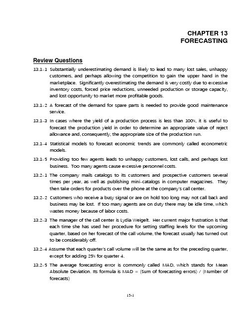
CHAPTER 13FORECASTINGReview Questions13.1-1 Substantially underestimating demand is likely to lead to many lost sales, unhappycustomers, and perhaps allowing the competition to gain the upper hand in the marketplace. Significantly overestimating the demand is very costly due to excessive inventory costs, forced price reductions, unneeded production or storage capacity, and lost opportunity to market more profitable goods.13.1-2 A forecast of the demand for spare parts is needed to provide good maintenanceservice.13.1-3 In cases where the yield of a production process is less than 100%, it is useful toforecast the production yield in order to determine an appropriate value of reject allowance and, consequently, the appropriate size of the production run.13.1-4 Statistical models to forecast economic trends are commonly called econometricmodels.13.1-5 Providing too few agents leads to unhappy customers, lost calls, and perhaps lostbusiness. Too many agents cause excessive personnel costs.13.2-1 The company mails catalogs to its customers and prospective customers severaltimes per year, as well as publishing mini-catalogs in computer magazines. They then take orders for products over the phone at the company’s call center.13.2-2 Customers who receive a busy signal or are on hold too long may not call back andbusiness may be lost. If too many agents are on duty there may be idle time, which wastes money because of labor costs.13.2-3 The manager of the call center is Lydia Weigelt. Her current major frustration is thateach time she has used her procedure for setting staffing levels for the upcoming quarter, based on her forecast of the call volume, the forecast usually has turned out to be considerably off.13.2-4 Assume that each quarter’s cal l volume will be the same as for the preceding quarter,except for adding 25% for quarter 4.13.2-5 The average forecasting error is commonly called MAD, which stands for MeanAbsolute Deviation. Its formula is MAD = (Sum of forecasting errors) / (Number of forecasts)13.2-6 MSE is the mean square error. Its formula is (Sum of square of forecasting errors) /(Number of forecasts).13.2-7 A time series is a series of observations over time of some quantity of interest.13.3-1 In general, the seasonal factor for any period of a year measures how that periodcompares to the overall average for an entire year.13.3-2 Seasonally adjusted call volume = (Actual call volume) / (Seasonal factor).13.3-3 Actual forecast = (Seasonal factor)(Seasonally adjusted forecast)13.3-4 The last-value forecasting method sometimes is called the naive method becausestatisticians consider it naive to use just a sample size of one when additional relevant data are available.13.3-5 Conditions affecting the CCW call volume were changing significantly over the pastthree years.13.3-6 Rather than using old data that may no longer be relevant, this method averages thedata for only the most recent periods.13.3-7 This method modifies the moving-average method by placing the greatest weighton the last value in the time series and then progressively smaller weights on the older values.13.3-8 A small value is appropriate if conditions are remaining relatively stable. A largervalue is needed if significant changes in the conditions are occurring relatively frequently.13.3-9 Forecast = α(Last Value) + (1 –α)(Last forecast). Estimated trend is added to thisformula when using exponential smoothing with trend.13.3-10 T he one big factor that drives total sales up or down is whether there are any hotnew products being offered.13.4-1 CB Predictor uses the raw data to provide the best fit for all these inputs as well asthe forecasts.13.4-2 Each piece of data should have only a 5% chance of falling below the lower line and a5% chance of rising above the upper line.13.5-1 The next value that will occur in a time series is a random variable.13.5-2 The goal of time series forecasting methods is to estimate the mean of theunderlying probability distribution of the next value of the time series as closely as possible.13.5-3 No, the probability distribution is not the same for every quarter.13.5-4 Each of the forecasting methods, except for the last-value method, placed at leastsome weight on the observations from Year 1 to estimate the mean for each quarter in Year 2. These observations, however, provide a poor basis for estimating the mean of the Year 2 distribution.13.5-5 A time series is said to be stable if its underlying probability distribution usuallyremains the same from one time period to the next. A time series is unstable if both frequent and sizable shifts in the distribution tend to occur.13.5-6 Since sales drive call volume, the forecasting process should begin by forecastingsales.13.5-7 The major components are the relatively stable market base of numerous small-niche products and each of a few major new products.13.6-1 Causal forecasting obtains a forecast of the quantity of interest by relating it directlyto one or more other quantities that drive the quantity of interest.13.6-2 The dependent variable is call volume and the independent variable is sales.13.6-3 When doing causal forecasting with a single independent variable, linear regressioninvolves approximating the relationship between the dependent variable and the independent variable by a straight line.13.6-4 In general, the equation for the linear regression line has the form y = a + bx. Ifthere is more than one independent variable, then this regression equation has a term, a constant times the variable, added on the right-hand side for each of these variables.13.6-5 The procedure used to obtain a and b is called the method of least squares.13.6-6 The new procedure gives a MAD value of only 120 compared with the old MADvalue of 400 with the 25% rule.13.7-1 Statistical forecasting methods cannot be used if no data are available, or if the dataare not representative of current conditions.13.7-2 Even when good data are available, some managers prefer a judgmental methodinstead of a formal statistical method. In many other cases, a combination of the two may be used.13.7-3 The jury of executive opinion method involves a small group of high-level managerswho pool their best judgment to collectively make a forecast rather than just the opinion of a single manager.13.7-4 The sales force composite method begins with each salesperson providing anestimate of what sales will be in his or her region.13.7-5 A consumer market survey is helpful for designing new products and then indeveloping the initial forecasts of their sales. It is also helpful for planning a marketing campaign.13.7-6 The Delphi method normally is used only at the highest levels of a corporation orgovernment to develop long-range forecasts of broad trends.13.8-1 Generally speaking, judgmental forecasting methods are somewhat more widelyused than statistical methods.13.8-2 Among the judgmental methods, the most popular is a jury of executive opinion.Manager’s opinion is a close second.13.8-3 The survey indicates that the moving-average method and linear regression are themost widely used statistical forecasting methods.Problems13.1 a) Forecast = last value = 39b) Forecast = average of all data to date = (5 + 17 + 29 + 41 + 39) / 5 = 131 / 5 =26c) Forecast = average of last 3 values = (29 + 41 + 39) / 3 = 109 / 3 = 36d) It appears as if demand is rising so the average forecasting method seemsinappropriate because it uses older, out-of-date data.13.2 a) Forecast = last value = 13b) Forecast = average of all data to date = (15 + 18 + 12 + 17 + 13) / 5 = 75 / 5 =15c) Forecast = average of last 3 values = (12 + 17 + 13) / 3 = 42 / 3 = 14d) The averaging method seems best since all five months of data are relevant indetermining the forecast of sales for next month and the data appears relativelystable.13.3MAD = (Sum of forecasting errors) / (Number of forecasts) = (18 + 15 + 8 + 19) / 4 = 60 / 4 = 15 MSE = (Sum of squares of forecasting errors) / (Number of forecasts) = (182 + 152 + 82 + 192) / 4 = 974 / 4 = 243.513.4 a) Method 1 MAD = (258 + 499 + 560 + 809 + 609) / 5 = 2,735 / 5 = 547Method 2 MAD = (374 + 471 + 293 + 906 + 396) / 5 = 2,440 / 5 = 488Method 1 MSE = (2582 + 4992 + 5602 + 8092 + 6092) / 5 = 1,654,527 / 5 = 330,905Method 2 MSE = (3742 + 4712 + 2932 + 9062 + 3962) / 5 = 1,425,218 / 5 = 285,044Method 2 gives a lower MAD and MSE.b) She can use the older data to calculate more forecasting errors and compareMAD for a longer time span. She can also use the older data to forecast theprevious five months to see how the methods compare. This may make her feelmore comfortable with her decision.13.5 a)b)c)d)13.6 a)b)This progression indicatesthat the state’s economy is improving with the unemployment rate decreasing from 8% to 7% (seasonally adjusted) over the four quarters.13.7 a)b) Seasonally adjusted value for Y3(Q4)=28/1.04=27,Actual forecast for Y4(Q1) = (27)(0.84) = 23.c) Y4(Q1) = 23 as shown in partb Seasonally adjusted value for Y4(Q1) = 23 / 0.84 = 27 Actual forecast for Y4(Q2) = (27)(0.92) = 25Seasonally adjusted value for Y4(Q2) = 25 / 0.92 = 27 Actual forecast for Y4(Q3) = (27)(1.20) = 33Seasonally adjusted value for Y4(Q3) = 33/1.20 = 27Actual forecast for Y4(Q4) = (27)(1.04) = 28d)13.8 Forecast = 2,083 – (1,945 / 4) + (1,977 / 4) = 2,09113.9 Forecast = 782 – (805 / 3) + (793 / 3) = 77813.10 Forecast = 1,551 – (1,632 / 10) + (1,532 / 10) = 1,54113.11 Forecast(α) = α(last value) + (1 –α)(last forecast)Forecast(0.1) = (0.1)(792) + (1 –0.1)(782) = 783 Forecast(0.3) = (0.3)(792) + (1 –0.3)(782) = 785 Forecast(0.5) = (0.5)(792) + (1 – 0.5)(782) = 78713.12 Forecast(α) = α(last value) + (1 –α)(last forecast)Forecast(0.1) = (0.1)(1,973) + (1 –0.1)(2,083) = 2,072 Forecast(0.3) = (0.3)(1,973) + (1 –0.3)(2,083) = 2,050 Forecast(0.5) = (0.5)(1,973) + (1 – 0.5)(2,083) = 2,02813.13 a) Forecast(year 1) = initial estimate = 5000Forecast(year 2) = α(last value) + (1 –α)(last forecast)= (0.25)(4,600) + (1 –0.25)(5,000) = 4,900 Forecast(year 3) = (0.25)(5,300) + (1 – 0.25)(4,900) = 5,000b) MAD = (400 + 400 + 1,000) / 3 = 600MSE = (4002 + 4002 + 1,0002) / 3 = 440,000c) Forecast(next year) = (0.25)(6,000) + (1 – 0.25)(5,000) = 5,25013.14 Forecast = α(last value) + (1 –α)(last forecast) + Estimated trendEstimated trend = β(Latest trend) + (1 –β)(Latest estimate of trend) Latest trend = α(Last value – Next-to-last value) + (1 –α)(Last forecast – Next-to-last forecast)Forecast(year 1) = Initial average + Initial trend = 3,900 + 700 = 4,600Forecast (year 2) = (0.25)(4,600) + (1 –0.25)(4,600)+(0.25)[(0.25)(4,600 –3900) + (1 –0.25)(4,600 –3,900)] + (1 –0.25)(700) = 5,300Forecast (year 3) = (0.25)(5,300) + (1 – 0.25)(5,300) + (0.25)[(0.25)(5,300 – 4,600) + (1 – 0.25)(5,300 – 4,600)]+(1 – 0.25)(700) = 6,00013.15 Forecast = α(last value) + (1 –α)(last forecast) + Estimated trendEstimated trend = β(Latest trend) + (1 –β)(Latest estimate of trend) Latest trend = α(Last value – Next-to-last value) + (1 –α)(Last forecast – Next-to-last forecast)Forecast = (0.2)(550) + (1 – 0.2)(540) + (0.3)[(0.2)(550 – 535) + (1 – 0.2)(540 –530)] + (1 – 0.3)(10) = 55213.16 Forecast = α(last value) + (1 –α)(last forecast) + Estimated trendEstimated trend = β(Latest trend) + (1 –β)(Latest estimate of trend) Latest trend = α(Last value – Next-to-last value) + (1 –α)(Last forecast – Next-to-last forecast)Forecast = (0.1)(4,935) + (1 – 0.1)(4,975) + (0.2)[(0.1)(4,935 – 4,655) + (1 – 0.1) (4,975 – 4720)] + (1 – 0.2)(240) = 5,21513.17 a) Since sales are relatively stable, the averaging method would be appropriate forforecasting future sales. This method uses a larger sample size than the last-valuemethod, which should make it more accurate and since the older data is stillrelevant, it should not be excluded, as would be the case in the moving-averagemethod.b)c)d)e) Considering the MAD values (5.2, 3.0, and 3.9, respectively), the averagingmethod is the best one to use.f) Considering the MSE values (30.6, 11.1, and 17.4, respectively), the averagingmethod is the best one to use.g) Unless there is reason to believe that sales will not continue to be relatively stable,the averaging method should be the most accurate in the future as well.13.18 Using the template for exponential smoothing, with an initial estimate of 24, thefollowing forecast errors were obtained for various values of the smoothing constant α:use.13.19 a) Answers will vary. Averaging or Moving Average appear to do a better job thanLast Value.b) For Last Value, a change in April will only affect the May forecast.For Averaging, a change in April will affect all forecasts after April.For Moving Average, a change in April will affect the May, June, and July forecast.c) Answers will vary. Averaging or Moving Average appear to do a slightly better jobthan Last Value.d) Answers will vary. Averaging or Moving Average appear to do a slightly better jobthan Last Value.13.20 a) Since the sales level is shifting significantly from month to month, and there is noconsistent trend, the last-value method seems like it will perform well. Theaveraging method will not do as well because it places too much weight on olddata. The moving-average method will be better than the averaging method butwill lag any short-term trends. The exponential smoothing method will also lagtrends by placing too much weight on old data. Exponential smoothing withtrend will likely not do well because the trend is not consistent.b)Comparing MAD values (5.3, 10.0, and 8.1, respectively), the last-value method is the best to use of these three options.Comparing MSE values (36.2, 131.4, and 84.3, respectively), the last-value method is the best to use of these three options.c) Using the template for exponential smoothing, with an initial estimate of 120, thefollowing forecast errors were obtained for various values of the smoothingconstant α:constant is appropriate.d) Using the template for exponential smoothing with trend, using initial estimates of120 for the average value and 10 for the trend, the following forecast errors wereobtained for various values of the smoothing constants α and β:constants is appropriate.e) Management should use the last-value method to forecast sales. Using thismethod the forecast for January of the new year will be 166. Exponentialsmoothing with trend with high smoothing constants (e.g., α = 0.5 and β = 0.5)also works well. With this method, the forecast for January of the new year will be165.13.21 a) Shift in total sales may be due to the release of new products on top of a stableproduct base, as was seen in the CCW case study.b) Forecasting might be improved by breaking down total sales into stable and newproducts. Exponential smoothing with a relatively small smoothing constant canbe used for the stable product base. Exponential smoothing with trend, with arelatively large smoothing constant, can be used for forecasting sales of each newproduct.c) Managerial judgment is needed to provide the initial estimate of anticipated salesin the first month for new products. In addition, a manger should check theexponential smoothing forecasts and make any adjustments that may benecessary based on knowledge of the marketplace.13.22 a) Answers will vary. Last value seems to do the best, with exponential smoothingwith trend a close second.b) For last value, a change in April will only affect the May forecast.For averaging, a change in April will affect all forecasts after April.For moving average, a change in April will affect the May, June, and July forecast.For exponential smoothing, a change in April will affect all forecasts after April.For exponential smoothing with trend, a change in April will affect all forecastsafter April.c) Answers will vary. last value or exponential smoothing seem to do better than theaveraging or moving average.d) Answers will vary. last value or exponential smoothing seem to do better than theaveraging or moving average.13.23 a) Using the template for exponential smoothing, with an initial estimate of 50, thefollowing MAD values were obtained for various values of the smoothing constantα:Choose αb) Using the template for exponential smoothing, with an initial estimate of 50, thefollowing MAD values were obtained for various values of the smoothing constantα:Choose αc) Using the template for exponential smoothing, with an initial estimate of 50, thefollowing MAD values were obtained for various values of the smoothing constantα:13.24 a)b)Forecast = 51.c) Forecast = 54.13.25 a) Using the template for exponential smoothing with trend, with an initial estimatesof 50 for the average and 2 for the trend and α = 0.2, the following MAD values were obtained for various values of the smoothing constant β:Choose β = 0.1b) Using the template for exponential smoothing with trend, with an initial estimatesof 50 for the average and 2 for the trend and α = 0.2, the following MAD valueswere obtained for various values of the smoothing constant β:Choose β = 0.1c) Using the template for exponential smoothing with trend, with an initial estimatesof 50 for the average and 2 for the trend and α = 0.2, the following MAD valueswere obtained for various values of the smoothing constant β:13.26 a)b)0.582. Forecast = 74.c) = 0.999. Forecast = 79.13.27 a) The time series is not stable enough for the moving-average method. Thereappears to be an upward trend.b)c)d)e) Based on the MAD and MSE values, exponential smoothing with trend should beused in the future.β = 0.999.f)For exponential smoothing, the forecasts typically lie below the demands.For exponential smoothing with trend, the forecasts are at about the same level as demand (perhaps slightly above).This would indicate that exponential smoothing with trend is the best method to usehereafter.13.2913.30 a)factors:b)c) Winter = (49)(0.550) = 27Spring = (49)(1.027) = 50Summer = (49)(1.519) = 74Fall = (49)(0.904) = 44d)e)f)g) The exponential smoothing method results in the lowest MAD value (1.42) and thelowest MSE value (2.75).13.31 a)b)c)d)e)f)g) The last-value method with seasonality has the lowest MAD and MSE value. Usingthis method, the forecast for Q1 is 23 houses.h) Forecast(Q2) = (27)(0.92) = 25Forecast(Q3) = (27)(1.2) = 32Forecast(Q4) = (27)(1.04) = 2813.32 a)b) The moving-average method with seasonality has the lowest MAD value. Using13.33 a)b)c)d) Exponential smoothing with trend should be used.e) The best values for the smoothing constants are α = 0.3, β = 0.3, and γ = 0.001.C28:C38 below.13.34 a)b)c)d)e) Moving average results in the best MAD value (13.30) and the best MSE value(249.09).f)MAD = 14.17g) Moving average performed better than the average of all three so it should beused next year.h) The best method is exponential smoothing with seasonality and trend, using13.35 a)••••••••••0100200300400500600012345678910S a l e sMonthb)c)••••••••••0100200300400500600012345678910S a l e sMonthd) y = 410.33 + (17.63)(11) = 604 e) y = 410.33 + (17.63)(20) = 763f) The average growth in sales per month is 17.63.13.36 a)•••01000200030004000500060000123A p p l i c a t i o n sYearb)•••01000200030004000500060000123A p p l i c a t i o n sYearc)d) y (year 4) = 3,900+ (700)(4) = 6,700 y (year 5) = 3,900 + (700)(5) = 7,400 y (year 6) = 3,900 + (700)(6) = 8,100 y (year 7) = 3,900 + (700)(7) =8,800y (year 8) = 3,900 + (700)(8) = 9,500e) It does not make sense to use the forecast obtained earlier of 9,500. Therelationship between the variable has changed and, thus, the linear regression that was used is no longer appropriate.f)•••••••0100020003000400050006000700001234567A p p l i c a t i o n sYeary =5,229 +92.9x y =5,229+(92.9)(8)=5,971the forecast that it provides for year 8 is not likely to be accurate. It does not make sense to continue to use a linear regression line when changing conditions cause a large shift in the underlying trend in the data.g)Causal forecasting takes all the data into account, even the data from before changing conditions cause a shift. Exponential smoothing with trend adjusts to shifts in the underlying trend by placing more emphasis on the recent data.13.37 a)••••••••••50100150200250300350400450500012345678910A n n u a l D e m a n dYearb)c)••••••••••50100150200250300350400450500012345678910A n n u a l D e m a n dYeard) y = 380 + (8.15)(11) = 470 e) y = 380 = (8.15)(15) = 503f) The average growth per year is 8.15 tons.13.38 a) The amount of advertising is the independent variable and sales is the dependentvariable.b)•••••0510*******100200300400500S a l e s (t h o u s a n d s o f p a s s e n g e r s )Amount of Advertising ($1,000s)c)•••••0510*******100200300400500S a l e s (t h o u s a n d s o f p a s s e n g e r s )Amount of Advertising ($1,000s)d) y = 8.71 + (0.031)(300) = 18,000 passengers e) 22 = 8.71 + (0.031)(x ) x = $429,000f) An increase of 31 passengers can be attained.13.39 a) If the sales change from 16 to 19 when the amount of advertising is 225, then thelinear regression line shifts below this point (the line actually shifts up, but not as much as the data point has shifted up).b) If the sales change from 23 to 26 when the amount of advertising is 450, then the linear regression line shifts below this point (the line actually shifts up, but not as much as the data point has shifted up).c) If the sales change from 20 to 23 when the amount of advertising is 350, then the linear regression line shifts below this point (the line actually shifts up, but not as much as the data point has shifted up).13.40 a) The number of flying hours is the independent variable and the number of wingflaps needed is the dependent variable.b)••••••024*********100200W i n g F l a p s N e e d e dFlying Hours (thousands)c)d)••••••024*********100200W i n g F l a p s N e e d e dFlying Hours (thousands)e) y = -3.38 + (0.093)(150) = 11f) y = -3.38 + (0.093)(200) = 1513.41 Joe should use the linear regression line y = –9.95 + 0.10x to develop a forecast forCase13.1 a) We need to forecast the call volume for each day separately.1) To obtain the seasonally adjusted call volume for the past 13 weeks, we firsthave to determine the seasonal factors. Because call volumes follow seasonalpatterns within the week, we have to calculate a seasonal factor for Monday,Tuesday, Wednesday, Thursday, and Friday. We use the Template for SeasonalFactors. The 0 values for holidays should not factor into the average. Leaving themblank (rather than 0) accomplishes this. (A blank value does not factor into theAVERAGE function in Excel that is used to calculate the seasonal values.) Using thistemplate (shown on the following page, the seasonal factors for Monday, Tuesday,Wednesday, Thursday, and Friday are 1.238, 1.131, 0.999, 0.850, and 0.762,respectively.2) To forecast the call volume for the next week using the last-value forecasting method, we need to use the Last Value with Seasonality template. To forecast the next week, we need only start with the last Friday value since the Last Value method only looks at the previous day.The forecasted call volume for the next week is 5,045 calls: 1,254 calls are received on Monday, 1,148 calls are received on Tuesday, 1,012 calls are received on Wednesday, 860 calls are received on Thursday, and 771 calls are received on Friday.3) To forecast the call volume for the next week using the averaging forecasting method, we need to use the Averaging with Seasonality template.The forecasted call volume for the next week is 4,712 calls: 1,171 calls are received on Monday, 1,071 calls are received on Tuesday, 945 calls are received on Wednesday, 804 calls are received on Thursday, and 721 calls are received onFriday.4) To forecast the call volume for the next week using the moving-average forecasting method, we need to use the Moving Averaging with Seasonality template. Since only the past 5 days are used in the forecast, we start with Monday of the last week to forecast through Friday of the next week.The forecasted call volume for the next week is 4,124 calls: 985 calls are received on Monday, 914 calls are received on Tuesday, 835 calls are received on Wednesday, 732 calls are received on Thursday, and 658 calls are received on Friday.5) To forecast the call volume for the next week using the exponential smoothing forecasting method, we need to use the Exponential with Seasonality template. We start with the initial estimate of 1,125 calls (the average number of calls on non-holidays during the previous 13 weeks).The forecasted call volume for the next week is 4,322 calls: 1,074 calls are received on Monday, 982 calls are received on Tuesday, 867 calls are received onWednesday, 737 calls are received on Thursday, and 661 calls are received on Friday.b) To obtain the mean absolute deviation for each forecasting method, we simplyneed to subtract the true call volume from the forecasted call volume for each day in the sixth week. We then need to take the absolute value of the five differences.Finally, we need to take the average of these five absolute values to obtain the mean absolute deviation.1) The spreadsheet for the calculation of the mean absolute deviation for the last-value forecasting method follows.This method is the least effective of the four methods because this method depends heavily upon the average seasonality factors. If the average seasonality factors are not the true seasonality factors for week 6, a large error will appear because the average seasonality factors are used to transform the Friday call volume in week 5 to forecasts for all call volumes in week 6. We calculated in part(a) that the call volume for Friday is 0.762 times lower than the overall average callvolume. In week 6, however, the call volume for Friday is only 0.83 times lower than the average call volume over the week. Also, we calculated that the call volume for Monday is 1.34 times higher than the overall average call volume. In Week 6, however, the call volume for Monday is only 1.21 times higher than the average call volume over the week. These differences introduce a large error.。
3.1-Forecasting
TS
Error = Actual – Forecast
MAD = ∑|Error| / n
16
Method 1: Tracking signal
Month 1 2 3 4 5 Actual 100 100 200 200 400 Forecast 60 130 200 270 340 Error 40 -30 0 -70 60 ∑|Error| 40 70 70 140 200 MAD 40 35 23 35 40 ∑(Error) 40 10 10 -60 0 TS 1.00 0.29 0.43 -1.71 0.00
2
Intended learning outcomes
Demand management
Describe the role of forecasts in demand management Know how to evaluate the accuracy of forecasting errors by computing MAD, MSE, and MAPE Use tracking signals to monitor a forecasting model’s performance List the major types of forecasting techniques and their limitations Compute simple exponential smoothing forecasts with and without trend adjustment Know the procedure and significance of choosing the appropriate parameters for different forecasting models Identify the optimal parameters of an exponential smoothing forecasting models
Models for Time Series and ForecastingPPT
to accompany
Introduction to Business Statistics
fourth edition, by Ronald M. Weiers
Presentation by Priscilla Chaffe-Stengel
© 2002 The Wadsworth Group
? = b0 + b1x y • Linear: ? = b + b x + b x2 • Quadratic: y 0 1 2
Trend Equations
? = the trend line estimate of y y x = time period b0, b1, and b2 are coefficients that are selected to minimize the deviations between the ? and the actual data values trend estimates y y for the past time periods. Regression methods are used to determine the best values for the coefficients.
• Trend equation • Moving average • Exponential smoothing
ቤተ መጻሕፍቲ ባይዱ
• Seasonal index • Ratio to moving average method • Deseasonalizing • MAD criterion • MSE criterion • Constructing an index using the CPI • Shifting the base of an index
Forecasting--预测分析模型

Chapter 5 ForecastingLearning ObjectivesStudents will be able to:1.Understand and know when to usevarious families of forecasting models.pare moving averages, exponentialsmoothing, and trend time-seriesmodels.3.Seasonally adjust data.4.Understand Delphi and otherqualitative decision-makingapproaches.pute a variety of error measures.Chapter Outline5.1Introduction5.2Types of Forecasts5.3Scatter Diagrams and TimeSeries5.4Measures of Forecast Accuracy 5.5Time-Series Forecasting Models 5.6Monitoring and ControllingForecasts5.7Using the Computer to ForecastIntroductionEight steps to forecasting:1.Determine the use of the forecast.2.Select the items or quantities to beforecasted.3.Determine the time horizon of theforecast.4.Select the forecasting model ormodels.5.Gather the data needed to make theforecast.6.Validate the forecasting model.7.Make the forecast.8.Implement the results.These steps provide a systematic way of initiating, designing, and implementing a forecasting system.Types of ForecastsMoving Average Exponential SmoothingTrend Projections Time-Series Methods:include historical data over a time intervalForecasting TechniquesNo single method is superiorDelphi Methods Jury of Executive Opinion Sales Force Composite Consumer Market SurveyQualitative Models :attempt to include subjective factorsCausal Methods:include a variety of factorsRegression Analysis Multiple RegressionDecompositionQualitative MethodsDelphi Methodinteractive group process consisting ofobtaining information from a group ofrespondents through questionnaires andsurveysJury of Executive Opinionobtains opinions of a small group of high-level managers in combination withstatistical modelsSales Force Compositeallows each sales person to estimate thesales for his/her region and then compiles the data at a district or national levelConsumer Market Surveysolicits input from customers or potential customers regarding their futurepurchasing plansScatter Diagrams050100150200250300350400450024681012Time (Years)A n n u a l S a l e sR a d i o sTelevisionsCom p a c t D i s c s Scatter diagrams are helpful whenforecasting time-series data because they depict the relationship between variables.Measures of ForecastAccuracy Forecast errors allow one to see how well the forecast model works and compare that model with other forecast models.Forecast error= actual value –forecast valueMeasures of Forecast Accuracy (continued)Measures of forecast accuracy include: Mean Absolute Deviation (MAD)Mean Squared Error (MSE)Mean Absolute Percent Error (MAPE)= ∑|forecast errors|n= ∑(errors)n=∑actualn100%error2Hospital Days –Forecast Error ExampleMs. Smith forecastedtotal hospitalinpatient days last year. Now that the actual data are known, she is reevaluatingher forecasting model. Compute the MAD, MSE, and MAPE for her forecast.Month Forecast Actual JAN250243 FEB320315 MAR275286 APR260256 MAY250241 JUN275298 JUL300292 AUG325333 SEP320326 OCT350378 NOV365382 DEC380396Hospital Days –Forecast Error ExampleForecastActual|error|error^2|error/actual|JAN 2502437490.03FEB 3203155250.02MAR 275286111210.04APR 2602564160.02MAY 2502419810.04JUN 275298235290.08JUL 3002928640.03AUG 3253338640.02SEP 3203266360.02OCT 350378287840.07NOV 365382172890.04DEC 380396162560.04AVERAGE11.83192.833.68MAD =MSE =MAPE = .0368*100=Decomposition of a Time-SeriesTime series can be decomposed into:Trend (T):gradual up or downmovement over timeSeasonality (S):pattern offluctuations above or below trendline that occurs every yearCycles(C):patterns in data thatoccur every several yearsRandom variations (R):“blips”inthe data caused by chance andunusual situationsComponents of Decomposition-150-5050150250350450550650012345Time (Years)D e m a n d TrendActual DataCyclicRandomDecomposition of Time-Series: Two ModelsMultiplicative model assumes demand is the product of the four components.demand = T * S * C * RAdditive model assumes demand is the summation of the four components.demand = T + S + C + RMoving Averages Moving average methods consist of computing an average of the most recent n data values for the time series and using this average for the forecast of the next period.Simple moving average =∑demand in previous n periodsnWallace Garden Supply’s Three-Month Moving AverageMonth ActualShedSalesThree-Month Moving AverageJanuary10 February12 March13April16 May19 June23 July26(10+12+13)/3 = 11 2/3 (12+13+16)/3 = 13 2/3 (13+16+19)/3 = 16 (16+19+23)/3 = 19 1/3Weighted MovingAveragesWeighted moving averages use weights to put more emphasis on recent periods.Weighted moving average =∑(weight for period n) (demand in period n)∑weightsCalculating Weighted Moving AveragesWeightsApplied PeriodLast month3Two months ago21Three months ago3*Sales last month +2*Sales two months ago +1*Sales threemonths ago6Sum of weightsWallace Garden ’s Weighted Three -Month Moving AverageMonthActual Shed SalesThree-Month Weighted Moving Average101213161923January February March April May June July26[3*13+2*12+1*10]/6 = 12 1/6[3*16+2*13+1*12]/6 =14 1/3[3*19+2*16+1*13]/6 = 17[3*23+2*19+1*16]/6 = 20 1/2Exponential SmoothingExponential smoothing is a type of moving average technique that involves little record keeping of past data.New forecast= previous forecast + α(previous actual –previous forecast)Mathematically this is expressed as:F t = F t-1 + α(Y t-1 -F t-1)F t-1= previous forecast α= smoothing constant F t = new forecastY t-1= previous period actualQtr ActualRounded Forecast using α=0.10 TonnageUnloaded11801752168176= 175.00+0.10(180-175) 3159175 =175.50+0.10(168-175.50) 4175173 =174.75+0.10(159-174.75) 5190173 =173.18+0.10(175-173.18) 6205175 =173.36+0.10(190-173.36) 7180178 =175.02+0.10(205-175.02) 8182178 =178.02+0.10(180-178.02) 9?179= 178.22+0.10(182-178.22)Qtr ActualRounded Forecast using α=0.50 TonnageUnloaded11801752168178 =175.00+0.50(180-175) 3159173 =177.50+0.50(168-177.50) 4175166 =172.75+0.50(159-172.75) 5190170 =165.88+0.50(175-165.88) 6205180 =170.44+0.50(190-170.44) 7180193 =180.22+0.50(205-180.22) 8182186 =192.61+0.50(180-192.61) 9?184 =186.30+0.50(182-186.30)Selecting a SmoothingConstantActualForecast witha = 0.10Absolute DeviationsForecast witha = 0.50Absolute Deviations180175517551681768178101591751617314175173216691901731717020205175301802518017821931318217841864MAD10.012To select the best smoothing constant, evaluate the accuracy of each forecasting model.The lowest MAD results from α= 0.10PM Computer: Moving Average ExamplePM Computer assembles customized personal computers from generic parts. The owners purchase generic computer parts in volume at a discount from a variety of sources whenever they see a good deal.It is important that they develop a good forecast of demand for their computers so they can purchase component parts efficiently.PM Computers: DataPeriod month actual demand1Jan372Feb403Mar414Apr375May456June507July438Aug479Sept56Compute a 2-month moving averageCompute a 3-month weighted average using weights of 4,2,1 for the past three months ofdataCompute an exponential smoothing forecast using α= 0.7Using MAD, what forecast is most accurate?PM Computers: Moving Average Solution2 monthMA Abs. Dev 3 month WMA Abs. Dev Exp.Sm.Abs. Dev37.0037.00 3.0038.50 2.5039.10 1.9040.50 3.5040.14 3.1440.43 3.4339.00 6.0038.57 6.4338.03 6.9741.009.0042.147.8642.917.0947.50 4.5046.71 3.7147.87 4.8746.500.5045.29 1.7144.46 2.5445.0011.0046.299.7146.249.7651.5051.5753.07MAD5.29 5.43 4.95 Exponential smoothing resulted in the lowest MAD.Simple exponential smoothing fails to respond to trends, so a more complex model is necessary with trend adjustment. Simple exponential smoothing -first-order smoothingTrend adjusted smoothing -second-order smoothingLow βgives less weight to morerecent trends, while high βgiveshigher weight to more recent trends.Forecast including trend (FIT t+1) = new forecast (F t ) + trend correction(T t )whereT t = (1 -β)T t-1 + β(F t –F t-1)T i = smoothed trend for period 1T i-1= smoothed trend for the preceding period β= trend smoothing constantF t = simple exponential smoothed forecast for period t F t-1= forecast for period t-1Trend ProjectionTrend projections are used to forecast time-series data that exhibit a linear trend.Least squares may be used to determine a trend projection for future forecasts. Least squares determines the trend line forecast by minimizing the mean squared error between the trend line forecasts and the actual observed values. The independent variable is the time period and the dependent variable is the actual observed value in the time series.Trend Projection(continued)The formula for the trend projection is:Y= b+ b X0 1where: Y = predicted valueb1 = slope of the trend lineb0 = interceptX = time period (1,2,3…n)Midwestern Manufacturing Trend Projection Example Midwestern Manufacturing Company’s demand for electrical generators over the period of 1996 –2000 is given below.Year Time Sales1996174199727919983801999490200051052001614220027122Midwestern Manufacturing CompanyTrend SolutionSUMMARY OUTPUTRegression StatisticsMultiple R0.89R Square0.80Adjusted R Square0.76Standard Error12.43Observations7.00ANOVAdf SS MS F Sign. F Regression 1.003108.043108.0420.110.01 Residual 5.00772.82154.56Total 6.003880.86Coefficients StandardError t Stat P-valueLower95%Intercept56.7110.51 5.400.0029.70 Time10.54 2.35 4.480.01 4.50 Sales = 56.71 + 10.54 (time)MidwesternManufacturing ’s Trend60708090100110120130140150160199319941995199619971998199920002001Forecast pointsTrend LineActual demand lineXy 54.1070.56+=Seasonal Variations Seasonal indices can be used to make adjustments in the forecast for seasonality.A seasonal index indicates how a particular season compares with an average season.The seasonal index can be found by dividing the average value for a particular season by the average of all the data.Eichler Supplies: Seasonal Index ExampleMonthSales DemandAverage Two-Year DemandAverageMonthly DemandSeasonal IndexYear 1Year28010090940.957758580940.851809085940.9049011010094 1.064Jan Feb Mar Apr May11513112394 1.309………………Total Average Demand 1,128Seasonal Index:= Average 2 -year demand/Average monthly demandSeasonal Variationswith TrendSteps of Multiplicative Time-Series Model pute the CMA for each pute seasonal ratio (observation/CMA).3.Average seasonal ratios to get seasonal indices.4.If seasonal indices do not add to thenumber of seasons, multiply each index by (number of seasons)/(sum of the indices).Centered Moving Average (CMA)is an approach that prevents a variation due to trend from being incorrectly interpreted as a variation due to the season.Turner Industries Seasonal Variations with TrendTurner Industries’sales figures are shown below with the CMA andseasonal ratio.Year Quarter Sales CMA Seasonal Ratio1110821253150132 1.1364141134.125 1.051 21116136.3750.851234138.8750.9653159141.125 1.1274152143 1.063 31123145.1250.8482142147.1870.9631684165CMA (qtr 3 / yr 1 ) = .5(108) + 125 + 150 + 141+ .5(116)4Seasonal Ratio = Sales Qtr 3 = 150CMA 132Decomposition Method with Trend and Seasonal Components Decomposition is the process of isolating linear trend and seasonal factors to develop more accurate forecasts.There are five steps to decomposition:pute the seasonal index for eachseason.2.Deseasonalize the data by dividingeach number by its seasonal index.pute a trend line with thedeseasonalized data.e the trend line to forecast.5.Multiply the forecasts by the seasonalindex.Turner Industries has noticed a trend in quarterly sales figures. There is also aseasonal component. Below is the seasonal index and deseasonalized sales data.Yr Qtr Sales Seasonal Index DesasonalizedSales 111080.85127.05921250.96130.2083150 1.13132.7434141 1.06133.019211160.85136.47121340.96139.5833159 1.13140.7084152 1.06143.396311230.85144.70621420.96147.9173168 1.13148.67341651.06155.660*•This value is derived by averaging the season rations for each quarter.Refer to slide 5-37.Seasonal Index for Qtr 1 =0.851+0.848 = 0.8521080.85=Using the deseasonalized data, the following trend line was computed: SUMMARY OUTPUTRegression StatisticsMultiple R0.98981389R Square0.97973154Adjusted R Squar0.9777047Standard Error 1.26913895Observations12ANOVAdf SS MS F ignificance F Regression1778.5826246778.5826246483.37748.49E-10 Residual1016.10713664 1.610713664Total11794.6897613Coefficients Standard Error t Stat P-value Lower 95% Intercept124.780.781101025159.8320597 2.26E-18123.1046 Time 2.340.1061307321.985846048.49E-10 2.0969Sales = 124.78 + 2.34XTurner Industries: Decomposition Method Using the trend line, the following forecast was computed:Sales = 124.78 + 2.34XFor period 13 (quarter 1/ year 4):Sales = 124.78 + 2.34 (13)= 155.2 (before seasonality adjustment) After seasonality adjustment:Sales = 155.2 (0.85) = 131.92Seasonal index for quarter 1Multiple Regression with Trend and Seasonal Components Multiple regression can be used to develop an additive decomposition model.One independent variable is time. Seasons are represented by dummy independent variables.Y = a + b X + b X + b X + b X Where X = time period X = 1 if quarter 2= 0 otherwiseX = 1 if quarter 3= 0 otherwiseX = 1 if quarter 4= 0 otherwise1 12 23 34 41234Monitoring and Controlling Forecasts n |errors forecast |Σ MAD MAD i) period in demand forecast i period in demand Σ(actual MADRSFE gnal TrackingSi =−==whereTracking signals measure how well predictions fit actual data.Monitoring and Controlling Forecasts。
ARIMA(预测时间序列的模型)

ARIMA(预测时间序列的模型)Autoregressive integrated moving average(⼀种预测时间序列的模型) ARIMA In statistics and econometrics, and in particular in time series analysis, an autoregressive integrated moving average (ARIMA) model is a generalisation of an autoregressive moving average (ARMA) model. These models are fitted to time series data either to better understand the data or to predict future points in the series. They are applied in some cases where data show evidence of non-stationarity, where an initial differencing step (corresponding to the "integrated" part of the model) can be applied to remove the non-stationarity.The model is generally referred to as an ARIMA(p,d,q) model where p, d, and q are integers greater than or equal to zero and refer to the order of the autoregressive, integrated, and moving average parts of the model respectively. ARIMA models form an important part of the Box-Jenkins approach to time-series modelling. When one of the terms is zero, it's usual to drop AR, I or MA. For example, an I(1) model is ARIMA(0,1,0), and a MA(1) model is ARIMA(0,0,1).Contents[hide]1 Definition2 Forecasts using ARIMA models3 Examples4 Implementations in statistics packages5 See also6 References7 External linksDefinitionGiven a time series of data Xt where t is an integer index and the Xt are real numbers, then an ARMA(p,q) model is given by: where L is the lag operator, the αi are the parameters of the autoregressive part of the model, the θi are the parameters of the moving average part and the are error terms. The error terms are generally assumed to be independent,identically distributed variables sampled from a normal distribution with zero mean.Assume now that the polynomial has a unitary root of multiplicity d. Then it can be rewritten as:An ARIMA(p,d,q) process expresses this polynomial factorisation property, and is given by:a nd thus can be thought as a particular case of an ARMA(p+d,q) process having the auto-regressive polynomial with some roots in the unity. For this reason every ARIMA model withd>0 is not wide sense stationary.Forecasts using ARIMA modelsARIMA models are used for observable non-stationary processes Xt that have some clearly identifiable trends:constant trend (i.e. a non-zero average) leads to d = 1linear trend (i.e. a linear growth behavior) leads to d = 2quadratic trend (i.e. a quadratic growth behavior) leads to d = 3In these cases the ARIMA model can be viewed as a "cascade" of two models. The first is non-stationary:while the second is wide-sense stationary:Now standard forecasts techniques can be formulated for the process Yt, and then (having the sufficient number of initial conditions) Xt can be forecasted via opportune integration steps.[edit]ExamplesSome well-known special cases arise naturally. For example, an ARIMA(0,1,0) model is given by:which is simply a random walk.A number of variations on the ARIMA model are commonly used. For example, if multiple time seriesare used then the Xt can be thought of as vectors and a VARIMA model may be appropriate. Sometimesa seasonal effect is suspected in the model. For example, consider a model of daily road traffic volumes. Weekends clearly exhibit different behaviour from weekdays. In this case it is often considered better touse a SARIMA (seasonal ARIMA) model than to increase the order of the AR or MA parts of the model.If the time-series is suspected to exhibit long-range dependence then the d parameter may be replaced by certain non-integer values in an autoregressive fractionally integrated moving average model, which isalso called a Fractional ARIMA (FARIMA or ARFIMA) model.[edit]Implementations in statistics packagesIn R, the stats package includes an arima function. The function is documented in "ARIMAModelling of Time Series". Besides the ARIMA(p,d,q) part, the function also includes seasonalfactors, an intercept term, and exogenous variables (xreg, called "external regressors").[edit]See alsoAutocorrelationARMAX-12-ARIMAPartial autocorrelation[edit]ReferencesMills, Terence C. Time Series Techniques for Economists. Cambridge University Press, 1990.Percival, Donald B. and Andrew T. Walden. Spectral Analysis for Physical Applications.Cambridge University Press, 1993.Autoregressive integrated moving average (ARIMA) is one of the popular linear models in time series forecasting。
现代物流-英文版测试题-第七章需求管理、订单管理
TEST BANKCHAPTER 7: DEMAND MANAGEMENT, ORDER MANAGEMENTAND CUSTOMER SERVICEMultiple Choice Questions (correct answers are bolded)1. The creation across the supply chain and its markets of a coordinated flow of demand is the definition of ___________.a. order cycleb. order managementc. demand managementd. supply chain management[LO 7.1: To explain demand management and demand forecasting models; Easy; Concept; AACSB Category 3: Analytical thinking]2. ___________ refers to finished goods that are produced prior to receiving a customer order.a. Make-to-stockb. Supply managementc. Make-to-orderd. Speculation[LO 7.1: To explain demand management and demand forecasting models; Easy; Concept; AACSB Category 3: Analytical thinking]3. ___________ refers to finished goods that are produced after receiving a customer order.a. Make-to-stockb. Supply managementc. Make-to-orderd. Postponement[LO 7.1: To explain demand management and demand forecasting models; Easy; Concept; AACSB Category 3: Analytical thinking]4. Which of the following is not a basic type of demand forecasting model?a. exponential smoothingb. cause and effectc. judgmentald. time series[LO 7.1: To explain demand management and demand forecasting models; Moderate; Synthesis; AACSB Category 3: Analytical thinking]5. Surveys and analog techniques are examples of ___________ forecasting.a. cause and effectb. time seriesc. exponential smoothingd. judgmental[LO 7.1: To explain demand management and demand forecasting models; Moderate; Application; AACSB Category 3: Analytical thinking]6. An underlying assumption of ___________ forecasting is that future demand is dependent on past demand.a. trial and errorb. time seriesc. judgmentald. cause and effect[LO 7.1: To explain demand management and demand forecasting models; Moderate; Concept; AACSB Category 3: Analytical thinking]7. Which forecasting technique assumes that one or more factors are related to demand and that this relationship can be used to estimate future demand?a. exponential smoothingb. judgmentalc. cause and effectd. time series[LO 7.1: To explain demand management and demand forecasting models; Moderate; Concept; AACSB Category 3: Analytical thinking]8. Which forecasting technique tends to be appropriate when there is little or no historical data?a. exponential smoothingb. judgmentalc. time seriesd. cause and effect[LO 7.1: To explain demand management and demand forecasting models; Moderate; Application; AACSB Category 3: Analytical thinking]9. ___________ suggests that supply chain partners will be working from a collectively agreed-to single demand forecast number as opposed to each member working off its own demand forecast projection.a. Supply chain orientationb. Collaborative planning, forecasting, and replenishment (CPFR) conceptc. Order managementd. Supply chain analytics[LO 7.1: To explain demand management and demand forecasting models; Easy; Concept; AACSB Category 3: Analytical thinking]10. ___________ refers to the management of various activities associated with the order cycle.a. Logisticsb. Order processingc. Demand managementd. Order management[LO 7.2: To examine the order cycle and its four components; Easy; Concept; AACSB Category3: Analytical thinking]11. The order cycle is ___________.a. the time that it takes for a check to clearb. the time that it takes from when a customer places an order until the selling firm receives the orderc. also called the replenishment cycled. also called the vendor cycle[LO 7.2: To examine the order cycle and its four components; Moderate; Concept; AACSB Category3: Analytical thinking]12. The order cycle is composed of each of the following except:a. order retrieval.b. order delivery.c. order picking and assembly.d. order transmittal.[LO 7.2: To examine the order cycle and its four components; Difficult; Synthesis; AACSB Category 3: Analytical thinking]13. Which of the following statements is false?a. Some organizations have expanded the order management concept to include the length of time it takes for an organization to receive payment for an order.b. The order cycle should be analyzed in terms of total cycle time and cycle time variability.c. Order management has been profoundly impacted by advances in information systems.d. Order management is synonymous with order cycle.[LO 7.2: To examine the order cycle and its four components; Difficult; Synthesis; AACSB Category 3: Analytical thinking]14. Order transmittal is ___________.a. the series of events that occurs from the time a customer places an order and the time the customer receives the orderb. the series of events that occurs between the time a customer places an order and the time the seller receives the orderc. the series of events that occurs between the time a customer perceives the need for a product and the time the seller receives the orderd. the series of events that occurs between the time a customer places an order and the time the order cycle begins[LO 7.2: To examine the order cycle and its four components; Moderate; Concept; AACSB Category 3: Analytical thinking]15. In general, there are ___________ possible ways to transmit orders.a. threeb. fourc. fived. six[LO 7.2: To examine the order cycle and its four components; Moderate; Application; AACSB Category 3: Analytical thinking]16. ___________ and electronic ordering are order transmittal techniques that have emerged over the last 30 years.a. In-personb. Mailc. Faxd. Telephone[LO 7.2: To examine the order cycle and its four components; Easy; Application; AACSB Category 3: Analytical thinking]17. What is the second phase of the order cycle?a.order transmittalb.order processingc.order picking and assemblyd.order delivery[LO 7.2: To examine the order cycle and its four components; Moderate; Synthesis; AACSB Category 3: Analytical thinking]18. ___________ refers to the time from when the seller receives an order until an appropriate location is authorized to fill the order.a. Order processingb. Order cyclec. Order managementd. Order transmittal[LO 7.2: To examine the order cycle and its four components; Moderate; Concept; AACSB Category 3: Analytical thinking]19. Classifying orders according to pre-established guidelines so that a company can prioritize how orders are to be filled refers to ___________.a. order fill rateb. order managementc. order processingd. order triage[LO 7.2: To examine the order cycle and its four components; Moderate; Concept; AACSB Category 3: Analytical thinking]20. Order picking and assembly is ___________.a. the final stage of the order cycleb. the most important component of the order cyclec. the order cycle component that follows order processingd. the order cycle component that follows order transmittal[LO 7.2: To examine the order cycle and its four components; Moderate; Synthesis; AACSB Category 3: Analytical thinking]21. The text suggests that ___________ often represents the best opportunity to improve the effectiveness and efficiency of an order cycle.a. order transmittalb. order picking and assemblyc. order deliveryd. order processing[LO 7.2: To examine the order cycle and its four components; Difficult; Synthesis; AACSB Category 3: Analytical thinking]22. Which of the following is not a characteristic of contemporary voice-based order picking systems?a. easily disrupted by other noisesb. better voice qualityc. more powerfuld. less costly[LO 7.2: Order Management; Difficult; Synthesis; AACSB Category 3: Analytical thinking]23. Which of the following is not a benefit of voice-based order picking?a. fewer picking errorsb. improved productivityc. minimal training time to learn the technologyd. fewer employee accidents[LO 7.2: To examine the order cycle and its four components; Difficult; Synthesis; AACSB Category 3: Analytical thinking]24. The final phase of the order cycle is called order ___________.a. picking and assemblyb. deliveryc. receivingd. replenishment[LO 7.2: To examine the order cycle and its four components; Moderate; Synthesis; AACSB Category 3: Analytical thinking]25. The time span within which an order must arrive refers to ___________.a. transit time reliabilityb. order deliveryc. delivery windowd. transit time[LO 7.2: To examine the order cycle and its four components; Moderate; Concept; AACSB Category 3: Analytical thinking]26. A commonly used rule of thumb is that it costs approximately ___________ times as much to get a new customer as it does to keep an existing customer.a. threeb. fourc. fived. six[LO 7.3: To understand the four dimensions of customer service as they pertain to logistics; Moderate; Application; AACSB Category 3: Analytical thinking]27. An unhappy customer will tell ___________ other people about her/his unhappiness.a. sevenb. ninec. twelved. fifteen[LO 7.3: To understand the four dimensions of customer service as they pertain to logistics; Moderate; Application; AACSB Category 3: Analytical thinking]28. The ability of logistics management to satisfy users in terms of time, dependability, communication, and convenience is the definition of ___________.a. customer serviceb. the order cyclec. a perfect orderd. customer satisfaction[LO 7.3: To understand the four dimensions of customer service as they pertain to logistics; Moderate; Concept; AACSB Category 3: Analytical thinking]29. The order cycle is an excellent example of the ___________ dimension of customer service.a. timeb. conveniencec. dependabilityd. communication[LO 7.3: To understand the four dimensions of customer service as they pertain to logistics; Moderate; Application; AACSB Category 3: Analytical thinking]30. The percentage of orders that can be completely and immediately filled from existing stock is the ___________ rate.a. optimal inventoryb. order cyclec. perfect orderd. order fill[LO 7.3: To understand the four dimensions of customer service as they pertain to logistics; Easy; Concept; AACSB Category 3: Analytical thinking]31. What component of customer service focuses on the ease of doing business with a seller?a. convenienceb. dependabilityc. timed. communication[LO 7.3: To understand the four dimensions of customer service as they pertain to logistics; Easy; Concept; AACSB Category 3: Analytical thinking]32. What are multichannel marketing systems?a. channels that have multiple intermediaries between the producer and the consumerb. separate marketing channels that serve an individual customerc. the same thing as horizontal marketing systemsd. channels that combine horizontal and vertical marketing systems[LO 7.3: To understand the four dimensions of customer service as they pertain to logistics; Moderate; Concept; AACSB Category 3: Analytical thinking]33. Objectives should be SMART—that is, ___________, measurable, achievable, realistic, and timely.a. specificb. strategicc. staticd. striving[LO 7.4: To familiarize you with select managerial issues associated with customer service; Moderate; Application; AACSB Category 3: Analytical thinking]34. Which of the following statements is false?a. Goals tend to be broad, generalized statements regarding the overall results that the firm is trying to achieve.a. Objectives are more specific than goals.c. A central element to the establishment of customer service goals and objectives is determining the customer’s viewpoint.d. Objectives should be specific, measurable, achievable, and responsive.[LO 7.4: To familiarize you with select managerial issues associated with customer service; Difficult; Synthesis; AACSB Category 3: Analytical thinking]35. ___________ refers to a process that continuously identifies, understands, and adapts outstanding processes inside and outside an organization.a. Environmental scanningb. Quality managementc. Benchmarkingd. Continuous improvement[LO 7.4: To familiarize you with select managerial issues associated with customer service; Moderate; Concept; AACSB Category 3: Analytical thinking]36. ___________ is the process of taking corrective action when measurements indicate that the goals and objectives of customer service are not being achieved.a. Benchmarkingb. Leadershipc. Controld. Managing[LO 7.4: To familiarize you with select managerial issues associated with customer service; Moderate; Concept; AACSB Category 3: Analytical thinking]37. Which statement about measuring customer service is true?a. Firms should choose those aspects of customer service that are easiest to measure.b. Order cycle time is the most commonly used customer service measure.c. Firms should use as many customer service measures as they can.d. It is possible for organizations to use only one customer service metric.[LO 7.4: To familiarize you with select managerial issues associated with customer service; Difficult; Synthesis; AACSB Category 3: Analytical thinking]38. ___________ refers to the allocation of revenues and costs to customer segments or individual customers to calculate the profitability of the segments or customers.a. Customer profitability analysisb. Net present valuec. Customer lifetime valued. Activity-based costing (ABC)[LO 7.4: To familiarize you with select managerial issues associated with customer service; Easy; Concept; AACSB Category 3: Analytical thinking]39. Which of the following statements is false?a. The service recovery paradox is where a customer holds the responsible company in higher regard after the service recovery than if a service failure had not occurred in the first place.b. A set formula that companies should follow for service recovery exists.c. One service recovery guideline involves fair treatment for customers.d. Service recovery refers to a process for returning a customer to a state of satisfaction after a service or product has failed to live up to expectations.[LO 7.4: To familiarize you with select managerial issues associated with customer service; Difficult; Synthesis; AACSB Category 3: Analytical thinking]True-False Questions1.Demand management is important because efficient and effective supply chains have learnedto match both supply and demand. (True)[LO: Beginning of the chapter material; Moderate; Application; AACSB Category 3: Analytical thinking]2.In make-to-order situations, finished goods are produced after receiving a customer order.(True)[LO 7.1: To explain demand management and demand forecasting models; Easy; Concept; AACSB Category 3: Analytical thinking]3.Simple moving averages and weighted moving averages are examples of judgmentalforecasting. (False)[LO 7.1: To explain demand management and demand forecasting models; Moderate; Application; AACSB Category 3: Analytical thinking]4.Judgmental forecasting is appropriate when there is little or no historical data. (True)[LO 7.1: To explain demand management and demand forecasting models; Moderate; Application; AACSB Category 3: Analytical thinking]5.Forecasting accuracy refers to the relationship between the actual and forecasted demand.(True)[LO 7.1: To explain demand management and demand forecasting models; Easy; Concept; AACSB Category 3: Analytical thinking]6.Demand chain management is where supply chain partners share planning and forecastingdata to better match up supply and demand. (False)[LO 7.1: To explain demand management and demand forecasting models; Moderate; Concept; AACSB Category 3: Analytical thinking]7.In general terms, order management refers to management of the various activities associatedwith the order cycle. (True)[LO 7.2: To examine the order cycle and its four components; Easy; Concept; AACSB Category 3: Analytical thinking]8.The order cycle is usually the time from when a customer places an order to when the firmreceives the order. (False)[LO 7.2: To examine the order cycle and its four components; Moderate; Concept; AACSB Category 3: Analytical thinking]9.There are four possible ways to transmit orders. (False)[LO 7.2: To examine the order cycle and its four components; Moderate; Application; AACSB Category 3: Analytical thinking]10.Order information is checked for completeness and accuracy in the order processingcomponent of the order cycle. (True)[LO 7.2: To examine the order cycle and its four components; Moderate; Synthesis; AACSB Category 3: Analytical thinking]11.The order triage function refers to correcting mistakes that may occur with order picking.(False)[LO 7.2: To examine the order cycle and its four components; Moderate; Concept; AACSB Category 3: Analytical thinking]12.A commonsense approach is to fill an order from the facility location that is closest to thecustomer, with the idea that this should generate lower transportation costs as well as ashorter order cycle time. (True)[LO 7.2: To examine the order cycle and its four components; Easy; Application; AACSB Category 3: Analytical thinking]13.Order processing often represents the best opportunity to improve the effectiveness andefficiency of the order cycle. (False)[LO 7.2: To examine the order cycle and its four components; Moderate; Application; AACSB Category 3: Analytical thinking]14.Travel time accounts for a majority of an order picker’s total pick time. (True)[LO 7.2: To examine the order cycle and its four components; Moderate; Synthesis; AACSB Category 3: Analytical thinking]15.Pick-to-light technology is an order picking technique that has grown in popularity in recentyears. (True)[LO 7.2: To examine the order cycle and its four components; Moderate; Application; AACSB Category 3: Analytical thinking]16.Order retrieval is the final phase of the order cycle. (False)[LO 7.2: To examine the order cycle and its four components; Moderate; Synthesis; AACSB Category 3: Analytical thinking]17.A key change in the order delivery component of the order cycle is that more and moreshippers are emphasizing both the elapsed transit time and transit time variability. (True) [LO 7.2: To examine the order cycle and its four components; Moderate; Application; AACSB Category 3: Analytical thinking]18.It costs about five times as much to get a new customer as it does to keep an existingcustomer. (True)[LO 7.3: To understand the four dimensions of customer service as they pertain to logistics; Easy; Application; AACSB Category 3: Analytical thinking]19.Consumers are demanding about the same levels of service today as in years past. (False) [LO 7.3: To understand the four dimensions of customer service as they pertain to logistics; Moderate; Synthesis; AACSB Category 3: Analytical thinking]20.The increased use of vendor quality-control programs necessitates higher levels of customerservice. (True)[LO 7.3: To understand the four dimensions of customer service as they pertain to logistics; Moderate; Synthesis; AACSB Category 3: Analytical thinking]21.Customer service can be defined as the ability of logistics management to satisfy users interms of quality, dependability, communication, and convenience. (False)[LO 7.3: To understand the four dimensions of customer service as they pertain to logistics; Moderate; Concept; AACSB Category 3: Analytical thinking]22.Dependability consists of consistent order cycles, safe delivery, and complete delivery.(True)[LO 7.3: To understand the four dimensions of customer service as they pertain to logistics; Moderate; Synthesis; AACSB Category 3: Analytical thinking]panies today will not accept slower order cycles in exchange for higher order cycleconsistency. (False)[LO 7.3: To understand the four dimensions of customer service as they pertain to logistics; Moderate; Synthesis; AACSB Category 3: Analytical thinking]24.Order fill rate is the percentage of orders that can be completely and immediately filled fromexisting stock. (True)[LO 7.3: To understand the four dimensions of customer service as they pertain to logistics; Easy; Concept; AACSB Category 3: Analytical thinking]25.Text messaging and the Internet have lessened the need for telephone interaction and face-to-face contact between seller and customer. (False)[LO 7.3: To understand the four dimensions of customer service as they pertain to logistics; Moderate; Synthesis; AACSB Category 3: Analytical thinking]26.The convenience component of customer service focuses on the ease of doing business with aseller. (True)[LO 7.3: To understand the four dimensions of customer service as they pertain to logistics; Easy; Concept; AACSB Category 3: Analytical thinking]27.Today’s customer likes to have multiple purchasing options at her/his disposal, andorganizations have responded by developing hybrid marketing channels—that is, separate marketing channels to serve an individual customer. (False)[LO 7.3: To understand the four dimensions of customer service as they pertain to logistics; Moderate; Concept; AACSB Category 3: Analytical thinking]28.Goals are the means by which objectives are achieved. (False)[LO 7.4: To familiarize you with select managerial issues associated with customer service; Moderate; Concept; AACSB Category 3: Analytical thinking]29.Objectives should be specific, measurable, achievable, realistic, and timely. (True)[LO 7.4: To familiarize you with select managerial issues associated with customer service; Moderate; Synthesis; AACSB Category 3: Analytical thinking]30.Continuous improvement refers to a process that continuously identifies, understands, andadapts outstanding processes found inside and outside an organization. (False)[LO 7.4: To familiarize you with select managerial issues associated with customer service; Moderate; Concept; AACSB Category 3: Analytical thinking]31.Benchmarking should only involve numerical comparisons of relevant metrics. (False) [LO 7.4: To familiarize you with select managerial issues associated with customer service; Moderate; Synthesis; AACSB Category 3: Analytical thinking]32.The nature of the product can affect the level of customer service that should be offered.(True)[LO 7.4: To familiarize you with select managerial issues associated with customer service; Moderate; Synthesis; AACSB Category 3: Analytical thinking]33.A product just being introduced needs a different level of service support than one that is in amature or declining market stage. (True)[LO 7.4: To familiarize you with select managerial issues associated with customer service; Moderate; Synthesis; AACSB Category 3: Analytical thinking]34.Leadership is the process of taking corrective action when measurements indicate that thegoals and objectives of customer service are not being achieved. (False)[LO 7.4: To familiarize you with select managerial issues associated with customer service; Moderate; Concept; AACSB Category 3: Analytical thinking]35.The customer service metrics that are chosen should be relevant and important from thecustomer’s perspective. (True)[LO 7.4: To familiarize you with select managerial issues associated with customer service; Moderate; Synthesis; AACSB Category 3: Analytical thinking]36.It is possible for organizations to use only one customer service metric to measure customerservice. (True)[LO 7.4: To familiarize you with select managerial issues associated with customer service; Easy; Application; AACSB Category 3: Analytical thinking37.Customer profitability analysis explicitly recognizes that all customers are not the same andthat some customers are more valuable than others to an organization. (True)[LO 7.4: To familiarize you with select managerial issues associated with customer service; Moderate; Concept; AACSB Category 3: Analytical thinking]38.Customer profitability analysis is grounded in traditional accounting cost allocation methods.(False)[LO 7.4: To familiarize you with select managerial issues associated with customer service; Moderate; Application; AACSB Category 3: Analytical thinking]39.Poor customer experiences cost U.S. business in excess of $75 billion per year. (False) [LO 7.4: To familiarize you with select managerial issues associated with customer service; Moderate; Synthesis; AACSB Category 3: Analytical thinking]40.In the service recovery paradox, a customer holds the responsible company in higher regardafter the service than if a service failure had not occurred in the first place. (True)[LO 7.4: To familiarize you with select managerial issues associated with customer service; Moderate; Application; AACSB Category 3: Analytical thinking]。
- 1、下载文档前请自行甄别文档内容的完整性,平台不提供额外的编辑、内容补充、找答案等附加服务。
- 2、"仅部分预览"的文档,不可在线预览部分如存在完整性等问题,可反馈申请退款(可完整预览的文档不适用该条件!)。
- 3、如文档侵犯您的权益,请联系客服反馈,我们会尽快为您处理(人工客服工作时间:9:00-18:30)。
Seasonal Indexes - An Example
Season (Annual Quarter)
Index Value
I
84.5
II
102.3
III
95.5
IV
117.7
• If the trend value for Quarter I in the given year was 902, the value with seasonal fluctuation would be
• A centered moving average is a moving average such that the time period is at the center of the N time periods used to determine which values to average.
a = the smoothing constant, 0 a 1
• The larger a is, the closer the smoothed value will track the original data value. The smaller a is, the more
fluctuation is smoothed out.
If N is an even number, the techniques need to be adjusted to place the time period at the center of the averaged values. The number of time periods N is usually based on the number of periods in a seasonal cycle. The larger N is, the more fluctuation will be smoothed out.
I = irregular component, which reflects fluctuations that
are not systematic
© 2002 The Wadsworth Group
Trend Equations
• Linear: y? = b0 + b1x • Quadratic: y? = b0 + b1x + b2x2
• Fit a linear or quadratic trend equation to a time series.
• Smooth a time series with the centered moving average and exponential smoothing techniques.
© 2002 The Wadsworth Group
Chapter 18 - Learning Objectives
• Describe the trend, cyclical, seasonal, and irregular components of the time series model.
CHAPTER 18 Models for Time Series and
Forecasting
to accompany
Introduction to Business Statistics
fourth edition, by Ronald M. Weiers
Presentation by Priscilla Chaffe-Stengel Donald N. Stengel
1998, Quarter I
867
1998, Quarter II
899
• 3-Quarter Centered Moving Average for 1997, Quarter IV:
844
906 3
867
872 .3
• 4-Quarter Centered Moving Average for 1997, Quarter IV:
Seasonal Indexes
• A seasonal index is a factor that adjusts a trend value to compensate for typical seasonal fluctuation in that period of a seasonal cycle.
• Shifting the base of an index
© 2002 The Wadsworth Group
Classical Time Series Model
y=T•C•S•I
where y = observed value of the time series variable
T = trend component, which reflects the general tendency of the time series without fluctuations
y = T • S = 902 • 84.5% = 762.2
© 2002 The Wadsworth Group
Ratio to Moving Average Method
• A technique for developing a set of seasonal index values from the original time series.
y?= the trend line estimate of y
x = time period
b0, b1, and b2 are coefficients that are selected to minimize the deviations between the trend estimates y? and the actual data values y for the past time periods. Regression methods are used to determine the best values for the coefficients.
C = cyclical component, which reflects systematic fluctuations that are not calendar-related, such as business cycles
S = seasonal component, which reflects systematic fluctuations that are calendar-related, such as the day of the week or the month of the year
• Use MAD and MSE criteria to compare how well equations fit data.
• Use index numbers to compare business or economic measures over time.
© 2002 The Wadsworth Group
• A seasonal index is expressed as a percentage with a value of 100% corresponding to an average position in a seasonal cycle.
© 2002 The Wadsworth Group
0.5861844
906 4
867
0.5844
906
867 4
899
874 .25
© 2002 The Wadsworth Group
Expபைடு நூலகம்nential Smoothing
where
Et = a•yt + (1 – a) Et–1
Et = exponentially smoothed value for time period t Et–1 = exponentially smoothed value for time period t – 1 yt = actual time series value for time period t
• Moving average - a technique that replaces a data value with the average of that data value and neighboring data values.
• Exponential smoothing - a technique that replaces a data value with a weighted average of the actual data value and the value resulting from exponential smoothing for the previous time period.
• Moving average
• Exponential smoothing
• Seasonal index
• Ratio to moving average method
• Deseasonalizing
• MAD criterion
• MSE criterion
• Constructing an index using the CPI
Chapter 18 - Key Terms
• Time series
• Classical time series model
– Trend value – Cyclical component – Seasonal component – Irregular component
• Trend equation