Abstract Semi-supervised Feature Selection via Spectral Analysis
ACM SIGKDD数据挖掘及知识发现会议

ACM SIGKDD数据挖掘及知识发现会议1清华大学计算机系王建勇1、KDD概况ACM SIGKDD国际会议(简称KDD)是由ACM的数据挖掘及知识发现专委会[1]主办的数据挖掘研究领域的顶级年会。
它为来自学术界、企业界和政府部门的研究人员和数据挖掘从业者进行学术交流和展示研究成果提供了一个理想场所,并涵盖了特邀主题演讲(keynote presentations)、论文口头报告(oral paper presentations)、论文展板展示(poster sessions)、研讨会(workshops)、短期课程(tutorials)、专题讨论会(panels)、展览(exhibits)、系统演示(demonstrations)、KDD CUP赛事以及多个奖项的颁发等众多内容。
由于KDD的交叉学科性和广泛应用性,其影响力越来越大,吸引了来自统计、机器学习、数据库、万维网、生物信息学、多媒体、自然语言处理、人机交互、社会网络计算、高性能计算及大数据挖掘等众多领域的专家、学者。
KDD可以追溯到从1989年开始组织的一系列关于知识发现及数据挖掘(KDD)的研讨会。
自1995年以来,KDD已经以大会的形式连续举办了17届,论文的投稿量和参会人数呈现出逐年增加的趋势。
2011年的KDD会议(即第17届KDD 年会)共收到提交的研究论文(Research paper)714篇和应用论文(Industrial and Government paper)73篇,参会人数也达到1070人。
下面我们将就会议的内容、历年论文投稿及接收情况以及设置的奖项情况进行综合介绍。
此外,由于第18届KDD年会将于2012年8月12日至16日在北京举办,我们还将简单介绍一下KDD’12[4]的有关情况。
2、会议内容自1995年召开第1届KDD年会以来,KDD的会议内容日趋丰富且变的相对稳定。
其核心内容是以论文报告和展版(poster)的形式进行数据挖掘同行之间的学术交流和成果展示。
基于Fisher准则的半监督特征提取方法
基于Fisher准则的半监督特征提取方法郝伟;刘忠宝【摘要】Mass unlabeled data and a small quantity of labeled data exist in practice.To fully utilize the labeled and unlabeled da-ta,semi-supervised feature extraction method based on Fisher criterion (SFEM)was proposed based on the depth analysis of the traditional semi-supervised feature extraction methods.The adj acent graph was constructed,and the within-class scatter matrix and the between-class scatter matrix were redefined.Fisher criterion was used to ensure the samples in different classes apart from each parative experiments on several standard datasets verify the effectiveness of SFEM in solving the problem of semi-supervised feature extraction.%针对实际应用中得到的数据往往只有少量具有类别标签,大多数类属未知的情况,在Fisher准则的基础上,提出基于Fisher 准则的半监督特征提取方法SFEM.在构造邻接图的基础上,重新定义类内离散度矩阵和类间离散度矩阵,利用Fisher准则找到的最优投影方向满足类间离散度矩阵与类内离散度矩阵之比最大,保证样本能较好地分开.若干标准数据集上的仿真结果表明,SFEM在解决半监督特征提取问题上具有一定优势.【期刊名称】《计算机工程与设计》【年(卷),期】2017(038)001【总页数】4页(P238-241)【关键词】特征提取;半监督算法;费希尔准则;类内离散度;类间离散度【作者】郝伟;刘忠宝【作者单位】山西工商学院计算机信息工程学院,山西太原 030006;中北大学计算机与控制工程学院,山西太原 030051【正文语种】中文【中图分类】TP391非负矩阵分解(non-negative matrix factorization,NMF)是一种常见的特征提取方法,其保证样本降维后的特征非负[1,2]。
文献 (10)Semi-supervised and unsupervised extreme learning
Semi-supervised and unsupervised extreme learningmachinesGao Huang,Shiji Song,Jatinder N.D.Gupta,and Cheng WuAbstract—Extreme learning machines(ELMs)have proven to be an efficient and effective learning paradigm for pattern classification and regression.However,ELMs are primarily applied to supervised learning problems.Only a few existing research studies have used ELMs to explore unlabeled data. In this paper,we extend ELMs for both semi-supervised and unsupervised tasks based on the manifold regularization,thus greatly expanding the applicability of ELMs.The key advantages of the proposed algorithms are1)both the semi-supervised ELM (SS-ELM)and the unsupervised ELM(US-ELM)exhibit the learning capability and computational efficiency of ELMs;2) both algorithms naturally handle multi-class classification or multi-cluster clustering;and3)both algorithms are inductive and can handle unseen data at test time directly.Moreover,it is shown in this paper that all the supervised,semi-supervised and unsupervised ELMs can actually be put into a unified framework. This provides new perspectives for understanding the mechanism of random feature mapping,which is the key concept in ELM theory.Empirical study on a wide range of data sets demonstrates that the proposed algorithms are competitive with state-of-the-art semi-supervised or unsupervised learning algorithms in terms of accuracy and efficiency.Index Terms—Clustering,embedding,extreme learning ma-chine,manifold regularization,semi-supervised learning,unsu-pervised learning.I.I NTRODUCTIONS INGLE layer feedforward networks(SLFNs)have been intensively studied during the past several decades.Most of the existing learning algorithms for training SLFNs,such as the famous back-propagation algorithm[1]and the Levenberg-Marquardt algorithm[2],adopt gradient methods to optimize the weights in the network.Some existing works also use forward selection or backward elimination approaches to con-struct network dynamically during the training process[3]–[7].However,neither the gradient based methods nor the grow/prune methods guarantee a global optimal solution.Al-though various methods,such as the generic and evolutionary algorithms,have been proposed to handle the local minimum This work was supported by the National Natural Science Foundation of China under Grant61273233,the Research Fund for the Doctoral Program of Higher Education under Grant20120002110035and20130002130010, the National Key Technology R&D Program under Grant2012BAF01B03, the Project of China Ocean Association under Grant DY125-25-02,and Tsinghua University Initiative Scientific Research Program under Grants 2011THZ07132.Gao Huang,Shiji Song,and Cheng Wu are with the Department of Automation,Tsinghua University,Beijing100084,China(e-mail:huang-g09@;shijis@; wuc@).Jatinder N.D.Gupta is with the College of Business Administration,The University of Alabama in Huntsville,Huntsville,AL35899,USA.(e-mail: guptaj@).problem,they basically introduce high computational cost. One of the most successful algorithms for training SLFNs is the support vector machines(SVMs)[8],[9],which is a maximal margin classifier derived under the framework of structural risk minimization(SRM).The dual problem of SVMs is a quadratic programming and can be solved conveniently.Due to its simplicity and stable generalization performance,SVMs have been widely studied and applied to various domains[10]–[14].Recently,Huang et al.[15],[16]proposed the extreme learning machines(ELMs)for training SLFNs.In contrast to most of the existing approaches,ELMs only update the output weights between the hidden layer and the output layer, while the parameters,i.e.,the input weights and biases,of the hidden layer are randomly generated.By adopting squared loss on the prediction error,the training of output weights turns into a regularized least squares(or ridge regression)problem which can be solved efficiently in closed form.It has been shown that even without updating the parameters of the hidden layer,the SLFN with randomly generated hidden neurons and tunable output weights maintains its universal approximation capability[17]–[19].Compared to gradient based algorithms, ELMs are much more efficient and usually lead to better generalization performance[20]–[22].Compared to SVMs, solving the regularized least squares problem in ELMs is also faster than solving the quadratic programming problem in standard SVMs.Moreover,ELMs can be used for multi-class classification problems directly.The predicting accuracy achieved by ELMs is comparable with or even higher than that of SVMs[16],[22]–[24].The differences and similarities between ELMs and SVMs are discussed in[25]and[26], and new algorithms are proposed by combining the advan-tages of both models.In[25],an extreme SVM(ESVM) model is proposed by combining ELMs and the proximal SVM(PSVM).The ESVM algorithm is shown to be more accurate than the basic ELMs model due to the introduced regularization technique,and much more efficient than SVMs since there is no kernel matrix multiplication in ESVM.In [26],the traditional RBF kernel are replaced by ELM kernel, leading to an efficient algorithm with matched accuracy of SVMs.In the past years,researchers from variesfields have made substantial contribution to ELM theories and applications.For example,the universal approximation ability of ELMs has been further studied in a classification context[23].The gen-eralization error bound of ELMs has been investigated from the perspective of the Vapnik-Chervonenkis(VC)dimension theory and the initial localized generalization error model(LGEM)[27],[28].Varies extensions have been made to the basic ELMs to make it more efficient and more suitable for specific problems,such as ELMs for online sequential data [29]–[31],ELMs for noisy/missing data[32]–[34],ELMs for imbalanced data[35],etc.From the implementation aspect, ELMs has recently been implemented using parallel tech-niques[36],[37],and realized on hardware[38],which made ELMs feasible for large data sets and real time reasoning. Though ELMs have become popular in a wide range of domains,they are primarily used for supervised learning tasks such as classification and regression,which greatly limits their applicability.In some cases,such as text classification, information retrieval and fault diagnosis,obtaining labels for fully supervised learning is time consuming and expensive, while a multitude of unlabeled data are easy and cheap to collect.To overcome the disadvantage of supervised learning al-gorithms that they cannot make use of unlabeled data,semi-supervised learning(SSL)has been proposed to leverage both labeled and unlabeled data[39],[40].The SSL algorithms assume that the input patterns from both labeled and unlabeled data are drawn from the same marginal distribution.Therefore, the unlabeled data naturally provide useful information for exploring the data structure in the input space.By assuming that the input data follows some cluster structure or manifold in the input space,SSL algorithms can incorporate both la-beled and unlabeled data into the learning process.Since SSL requires less effort to collect labeled data and can offer higher accuracy,it has been applied to various domains[41]–[43].In some other cases where no labeled data are available,people may be interested in exploring the underlying structure of the data.To this end,unsupervised learning(USL)techniques, such as clustering,dimension reduction or data representation, are widely used to fulfill these tasks.In this paper,we extend ELMs to handle both semi-supervised and unsupervised learning problems by introducing the manifold regularization framework.Both the proposed semi-supervised ELM(SS-ELM)and unsupervised ELM(US-ELM)inherit the computational efficiency and the learn-ing capability of traditional pared with existing algorithms,SS-ELM and US-ELM are not only inductive (straightforward extension for out-of-sample examples at test time),but also can be used for multi-class classification or multi-cluster clustering directly.We test our algorithms on a variety of data sets,and make comparisons with other related algorithms.The results show that the proposed algorithms are competitive with state-of-the-art algorithms in terms of accuracy and efficiency.It is worth to mention that all the supervised,semi-supervised and unsupervised ELMs can actually be put into a unified framework,that is all the algorithms consist of two stages:1)random feature mapping;and2)output weights solving.Thefirst stage is to construct the hidden layer using randomly generated hidden neurons.This is the key concept in the ELM theory,which differs it from many existing feature learning methods.Generating feature mapping randomly en-ables ELMs for fast nonlinear feature learning and alleviates the problem of over-fitting.The second stage is to solve the weights between the hidden layer and the output layer, and this is where the main difference of supervised,semi-supervised and unsupervised ELMs lies.We believe that the unified framework for the three types of ELMs might provide us a new perspective to understand the underlying behavior of the random feature mapping in ELMs.The rest of the paper is organized as follows.In Section II,we give a brief review of related existing literature on semi-supervised and unsupervised learning.Section III and IV introduce the basic formulation of ELMs and the man-ifold regularization framework,respectively.We present the proposed SS-ELM and US-ELM algorithms in Sections V and VI.Experiment results are given in Section VII,and Section VIII concludes the paper.II.R ELATED WORKSOnly a few existing research studies on ELMs have dealt with the problem of semi-supervised learning or unsupervised learning.In[44]and[45],the manifold regularization frame-work was introduce into the ELMs model to leverage both labeled and unlabeled data,thus extended ELMs for semi-supervised learning.However,both of these two works are limited to binary classification problems,thus they haven’t explore the full power of ELMs.Moreover,both algorithms are only effective when the number of training patterns is more than the number of hidden neurons.Unfortunately,this condition is usually violated in semi-supervised learning since the training data is relatively scarce compared to the hidden neurons,whose number is commonly set to several hundreds or several thousands.Recently,a co-training approach have been proposed to train ELMs in a semi-supervised setting [46].In this algorithm,the labeled training sets are augmented gradually by moving a small set of most confidently predicted unlabeled data to the labeled set at each loop,and ELMs are trained repeatedly on the pseudo-labeled set.Since the algo-rithm need to train ELMs repeatedly,it introduces considerable extra computational cost.The proposed SS-ELM is related to a few other mani-fold assumption based semi-supervised learning algorithms, such as the Laplacian support vector machines(LapSVMs) [47],the Laplacian regularized least squares(LapRLS)[47], semi-supervised neural networks(SSNNs)[48],and semi-supervised deep embedding[49].It has been shown in these works that manifold regularization is effective in a wide range of domains and often leads to a state-of-the-art performance in terms of accuracy and efficiency.The US-ELM proposed in this paper are related to the Laplacian Eigenmaps(LE)[50]and spectral clustering(SC) [51]in that they both use spectral techniques for embedding and clustering.In all these algorithms,an affinity matrix is first built from the input patterns.The SC performs eigen-decomposition on the normalized affinity matrix,and then embeds the original data into a d-dimensional space using the first d eigenvectors(each row is normalized to have unit length and represents a point in the embedded space)corresponding to the d largest eigenvalues.The LE algorithm performs generalized eigen-decomposition on the graph Laplacian,anduses the d eigenvectors corresponding to the second through the(d+1)th smallest eigenvalues for embedding.When LE and SC are used for clustering,then k-means is adopted to cluster the data in the embedded space.Similar to LE and SC,the US-ELM are also based on the affinity matrix,and it is converted to solving a generalized eigen-decomposition problem.However,the eigenvectors obtained in US-ELM are not used for data representation directly,but are used as the parameters of the network,i.e.,the output weights.Note that once the US-ELM model is trained,it can be applied to any presented data in the original input space.In this way,US-ELM provide a straightforward way for handling new patterns without recomputing eigenvectors as in LE and SC.III.E XTREME LEARNING MACHINES Consider a supervised learning problem where we have a training set with N samples,{X,Y}={x i,y i}N i=1.Herex i∈R n i,y i is a n o-dimensional binary vector with only one entry(correspond to the class that x i belongs to)equal to one for multi-classification tasks,or y i∈R n o for regression tasks,where n i and n o are the dimensions of input and output respectively.ELMs aim to learn a decision rule or an approximation function based on the training data. Generally,the training of ELMs consists of two stages.The first stage is to construct the hidden layer using afixed number of randomly generated mapping neurons,which can be any nonlinear piecewise continuous functions,such as the Sigmoid function and Gaussian function given below.1)Sigmoid functiong(x;θ)=11+exp(−(a T x+b));(1)2)Gaussian functiong(x;θ)=exp(−b∥x−a∥);(2) whereθ={a,b}are the parameters of the mapping function and∥·∥denotes the Euclidean norm.A notable feature of ELMs is that the parameters of the hidden mapping functions can be randomly generated ac-cording to any continuous probability distribution,e.g.,the uniform distribution on(-1,1).This makes ELMs distinct from the traditional feedforward neural networks and SVMs. The only free parameters that need to be optimized in the training process are the output weights between the hidden neurons and the output nodes.By doing so,training ELMs is equivalent to solving a regularized least squares problem which is considerately more efficient than the training of SVMs or backpropagation algorithms.In thefirst stage,a number of hidden neurons which map the data from the input space into a n h-dimensional feature space (n h is the number of hidden neurons)are randomly generated. We denote by h(x i)∈R1×n h the output vector of the hidden layer with respect to x i,andβ∈R n h×n o the output weights that connect the hidden layer with the output layer.Then,the outputs of the network are given byf(x i)=h(x i)β,i=1,...,N.(3)In the second stage,ELMs aim to solve the output weights by minimizing the sum of the squared losses of the prediction errors,which leads to the following formulationminβ∈R n h×n o12∥β∥2+C2N∑i=1∥e i∥2s.t.h(x i)β=y T i−e T i,i=1,...,N,(4)where thefirst term in the objective function is a regularization term which controls the complexity of the model,e i∈R n o is the error vector with respect to the i th training pattern,and C is a penalty coefficient on the training errors.By substituting the constraints into the objective function, we obtain the following equivalent unconstrained optimization problem:minβ∈R n h×n oL ELM=12∥β∥2+C2∥Y−Hβ∥2(5)where H=[h(x1)T,...,h(x N)T]T∈R N×n h.The above problem is widely known as the ridge regression or regularized least squares.By setting the gradient of L ELM with respect toβto zero,we have∇L ELM=β+CH H T(Y−Hβ)=0(6) If H has more rows than columns and is of full column rank,which is usually the case where the number of training patterns are more than the number of the hidden neurons,the above equation is overdetermined,and we have the following closed form solution for(5):β∗=(H T H+I nhC)−1H T Y,(7)where I nhis an identity matrix of dimension n h.Note that in practice,rather than explicitly inverting the n h×n h matrix in the above expression,we can use Gaussian elimination to directly solve a set of linear equations in a more efficient and numerically stable manner.If the number of training patterns are less than the number of hidden neurons,then H will have more columns than rows, which often leads to an underdetermined least squares prob-lem.In this case,βmay have infinite number of solutions.To handle this problem,we restrictβto be a linear combination of the rows of H:β=H Tα(α∈R N×n o).Notice that when H has more columns than rows and is of full row rank,then H H T is invertible.Multiplying both side of(6) by(H H T)−1H,we getα+C(Y−H H Tα)=0,(8) This yieldsβ∗=H Tα∗=H T(H H T+I NC)−1Y(9)where I N is an identity matrix of dimension N. Therefore,in the case where training patterns are plentiful compared to the hidden neurons,we use(7)to compute the output weights,otherwise we use(9).IV.T HE MANIFOLD REGULARIZATION FRAMEWORK Semi-supervised learning is built on the following two assumptions:(1)both the label data X l and the unlabeled data X u are drawn from the same marginal distribution P X ;and (2)if two points x 1and x 2are close to each other,then the conditional probabilities P (y |x 1)and P (y |x 2)should be similar as well.The latter assumption is widely known as the smoothness assumption in machine learning.To enforce this assumption on the data,the manifold regularization framework proposes to minimize the following cost functionL m=12∑i,jw ij ∥P (y |x i )−P (y |x j )∥2,(10)where w ij is the pair-wise similarity between two patterns x iand x j .Note that the similarity matrix W =[w ij ]is usually sparse,since we only place a nonzero weight between two patterns x i and x j if they are close,e.g.,x i is among the k nearest neighbors of x j or x j is among the k nearest neighbors of x i .The nonzero weights are usually computed using Gaussian function exp (−∥x i −x j ∥2/2σ2),or simply fixed to 1.Intuitively,the formulation (10)penalizes large variation in the conditional probability P (y |x )when x has a small change.This requires that P (y |x )vary smoothly along the geodesics of P (x ).Since it is difficult to compute the conditional probability,we can approximate (10)with the following expression:ˆLm =12∑i,jw ij ∥ˆyi −ˆy j ∥2,(11)where ˆyi and ˆy j are the predictions with respect to pattern x i and x j ,respectively.It is straightforward to simplify the above expression in a matrix form:ˆL m =Tr (ˆY T L ˆY ),(12)where Tr (·)denotes the trace of a matrix,L =D −W isknown as the graph Laplacian ,and D is a diagonal matrixwith its diagonal elements D ii =l +u∑j =1w i,j .As discussed in [52],instead of using L directly,we can normalize it byD −12L D −12or replace it by L p (p is an integer),based on some prior knowledge.V.S EMI -SUPERVISED ELMIn the semi-supervised setting,we have few labeled data and plenty of unlabeled data.We denote the labeled data in the training set as {X l ,Y l }={x i ,y i }l i =1,and unlabeled dataas X u ={x i }ui =1,where l and u are the number of labeled and unlabeled data,respectively.The proposed SS-ELM incorporates the manifold regular-ization to leverage unlabeled data to improve the classification accuracy when labeled data are scarce.By modifying the ordinary ELM formulation (4),we give the formulation ofSS-ELM as:minβ∈R n h ×n o12∥β∥2+12l∑i =1C i ∥e i ∥2+λ2Tr (F T L F )s.t.h (x i )β=y T i −e T i ,i =1,...,l,f i =h (x i )β,i =1,...,l +u(13)where L ∈R (l +u )×(l +u )is the graph Laplacian built fromboth labeled and unlabeled data,and F ∈R (l +u )×n o is the output matrix of the network with its i th row equal to f (x i ),λis a tradeoff parameter.Note that similar to the weighted ELM algorithm (W-ELM)introduced in [35],here we associate different penalty coeffi-cient C i on the prediction errors with respect to patterns from different classes.This is because we found that when the data is skewed,i.e.,some classes have significantly more training patterns than other classes,traditional ELMs tend to fit the classes that having the majority of patterns quite well but fits other classes poorly.This usually leads to poor generalization performance on the testing set (while the prediction accuracy may be high,but the some classes are neglected).Therefore,we propose to alleviate this problem by re-weighting instances from different classes.Suppose that x i belongs to class t i ,which has N t i training patterns,then we associate e i with a penalty ofC i =C 0N t i.(14)where C 0is a user defined parameter as in traditional ELMs.In this way,the patterns from the dominant classes will not be over fitted by the algorithm,and the patterns from a class with less samples will not be neglected.We substitute the constraints into the objective function,and rewrite the above formulation in a matrix form:min β∈R n h×n o 12∥β∥2+12∥C 12( Y −Hβ)∥2+λ2Tr (βT H TL Hβ)(15)where Y∈R (l +u )×n o is the training target with its first l rows equal to Y l and the rest equal to 0,C is a (l +u )×(l +u )diagonal matrix with its first l diagonal elements [C ]ii =C i ,i =1,...,l and the rest equal to 0.Again,we compute the gradient of the objective function with respect to β:∇L SS −ELM =β+H T C ( Y−H β)+λH H T L H β.(16)By setting the gradient to zero,we obtain the solution tothe SS-ELM:β∗=(I n h +H T C H +λH H T L H )−1H TC Y .(17)As in Section III,if the number of labeled data is fewer thanthe number of hidden neurons,which is common in SSL,we have the following alternative solution:β∗=H T (I l +u +C H H T +λL L H H T )−1C Y .(18)where I l +u is an identity matrix of dimension l +u .Note that by settingλto be zero and the diagonal elements of C i(i=1,...,l)to be the same constant,(17)and (18)reduce to the solutions of traditional ELMs(7)and(9), respectively.Based on the above discussion,the SS-ELM algorithm is summarized as Algorithm1.Algorithm1The SS-ELM algorithmInput:The labeled patterns,{X l,Y l}={x i,y i}l i=1;The unlabeled patterns,X u={x i}u i=1;Output:The mapping function of SS-ELM:f:R n i→R n oStep1:Construct the graph Laplacian L from both X l and X u.Step2:Initiate an ELM network of n h hidden neurons with random input weights and biases,and calculate the output matrix of the hidden neurons H∈R(l+u)×n h.Step3:Choose the tradeoff parameter C0andλ.Step4:•If n h≤NCompute the output weightsβusing(17)•ElseCompute the output weightsβusing(18)return The mapping function f(x)=h(x)β.VI.U NSUPERVISED ELMIn this section,we introduce the US-ELM algorithm for unsupervised learning.In an unsupervised setting,the entire training data X={x i}N i=1are unlabeled(N is the number of training patterns)and our target is tofind the underlying structure of the original data.The formulation of US-ELM follows from the formulation of SS-ELM.When there is no labeled data,(15)is reduced tomin β∈R n h×n o ∥β∥2+λTr(βT H T L Hβ)(19)Notice that the above formulation always attains its mini-mum atβ=0.As suggested in[50],we have to introduce addtional constraints to avoid a degenerated solution.Specifi-cally,the formulation of US-ELM is given bymin β∈R n h×n o ∥β∥2+λTr(βT H T L Hβ)s.t.(Hβ)T Hβ=I no(20)Theorem1:An optimal solution to problem(20)is given by choosingβas the matrix whose columns are the eigenvectors (normalized to satisfy the constraint)corresponding to thefirst n o smallest eigenvalues of the generalized eigenvalue problem:(I nh +λH H T L H)v=γH H T H v.(21)Proof:We can rewrite the problem(20)asminβ∈R n h×n o,ββT Bβ=I no Tr(βT Aβ),(22)Algorithm2The US-ELM algorithmInput:The training data:X∈R N×n i;Output:•For embedding task:The embedding in a n o-dimensional space:E∈R N×n o;•For clustering task:The label vector of cluster index:y∈N N×1+.Step1:Construct the graph Laplacian L from X.Step2:Initiate an ELM network of n h hidden neurons withrandom input weights,and calculate the output matrix of thehidden neurons H∈R N×n h.Step3:•If n h≤NFind the generalized eigenvectors v2,v3,...,v no+1of(21)corresponding to the second through the n o+1smallest eigenvalues.Letβ=[ v2, v3,..., v no+1],where v i=v i/∥H v i∥,i=2,...,n o+1.•ElseFind the generalized eigenvectors u2,u3,...,u no+1of(24)corresponding to the second through the n o+1smallest eigenvalues.Letβ=H T[ u2, u3,..., u no+1],where u i=u i/∥H H T u i∥,i=2,...,n o+1.Step4:Calculate the embedding matrix:E=Hβ.Step5(For clustering only):Treat each row of E as a point,and cluster the N points into K clusters using the k-meansalgorithm.Let y be the label vector of cluster index for allthe points.return E(for embedding task)or y(for clustering task);where A=I nh+λH H T L H and B=H T H.It is easy to verify that both A and B are Hermitianmatrices.Thus,according to the Rayleigh-Ritz theorem[53],the above trace minimization problem attains its optimum ifand only if the column span ofβis the minimum span ofthe eigenspace corresponding to the smallest n o eigenvaluesof(21).Therefore,by stacking the normalized eigenvectors of(21)corresponding to the smallest n o generalized eigenvalues,we obtain an optimal solution to(20).In the algorithm of Laplacian eigenmaps,thefirst eigenvec-tor is discarded since it is always a constant vector proportionalto1(corresponding to the smallest eigenvalue0)[50].In theUS-ELM algorithm,thefirst eigenvector of(21)also leadsto small variations in embedding and is not useful for datarepresentation.Therefore,we suggest to discard this trivialsolution as well.Letγ1,γ2,...,γno+1(γ1≤γ2≤...≤γn o+1)be the(n o+1)smallest eigenvalues of(21)and v1,v2,...,v no+1be their corresponding eigenvectors.Then,the solution to theoutput weightsβis given byβ∗=[ v2, v3,..., v no+1],(23)where v i=v i/∥H v i∥,i=2,...,n o+1are the normalizedeigenvectors.If the number of labeled data is fewer than the numberTABLE ID ETAILS OF THE DATA SETS USED FOR SEMI-SUPERVISED LEARNINGData set Class Dimension|L||U||V||T|G50C2505031450136COIL20(B)2102440100040360USPST(B)225650140950498COIL2020102440100040360USPST1025650140950498of hidden neurons,problem(21)is underdetermined.In this case,we have the following alternative formulation by using the same trick as in previous sections:(I u+λL L H H T )u=γH H H T u.(24)Again,let u1,u2,...,u no +1be generalized eigenvectorscorresponding to the(n o+1)smallest eigenvalues of(24), then thefinal solution is given byβ∗=H T[ u2, u3,..., u no +1],(25)where u i=u i/∥H H T u i∥,i=2,...,n o+1are the normal-ized eigenvectors.If our task is clustering,then we can adopt the k-means algorithm to perform clustering in the embedded space.We summarize the proposed US-ELM in Algorithm2. Remark:Comparing the supervised ELM,the semi-supervised ELM and the unsupervised ELM,we can observe that all the algorithms have two similar stages in the training process,that is the random feature learning stage and the out-put weights learning stage.Under this two-stage framework,it is easy tofind the differences and similarities between the three algorithms.Actually,all the algorithms share the same stage of random feature learning,and this is the essence of the ELM theory.This also means that no matter the task is a supervised, semi-supervised or unsupervised learning problem,we can always follow the same step to generate the hidden layer. The differences of the three types of ELMs lie in the second stage on how the output weights are computed.In supervised ELM and SS-ELM,the output weights are trained by solving a regularized least squares problem;while the output weights in the US-ELM are obtained by solving a generalized eigenvalue problem.The unified framework for the three types of ELMs might provide new perspectives to further develop the ELM theory.VII.E XPERIMENTAL RESULTSWe evaluated our algorithms on wide range of semi-supervised and unsupervised parisons were made with related state-of-the-art algorithms, e.g.,Transductive SVM(TSVM)[54],LapSVM[47]and LapRLS[47]for semi-supervised learning;and Laplacian Eigenmap(LE)[50], spectral clustering(SC)[51]and deep autoencoder(DA)[55] for unsupervised learning.All algorithms were implemented using Matlab R2012a on a2.60GHz machine with4GB of memory.TABLE IIIT RAINING TIME(IN SECONDS)COMPARISON OF TSVM,L AP RLS,L AP SVM AND SS-ELMData set TSVM LapRLS LapSVM SS-ELMG50C0.3240.0410.0450.035COIL20(B)16.820.5120.4590.516USPST(B)68.440.9210.947 1.029COIL2018.43 5.841 4.9460.814USPST68.147.1217.259 1.373A.Semi-supervised learning results1)Data sets:We tested the SS-ELM onfive popular semi-supervised learning benchmarks,which have been widely usedfor evaluating semi-supervised algorithms[52],[56],[57].•The G50C is a binary classification data set of which each class is generated by a50-dimensional multivariate Gaus-sian distribution.This classification problem is explicitlydesigned so that the true Bayes error is5%.•The Columbia Object Image Library(COIL20)is a multi-class image classification data set which consists1440 gray-scale images of20objects.Each pattern is a32×32 gray scale image of one object taken from a specific view.The COIL20(B)data set is a binary classification taskobtained from COIL20by grouping thefirst10objectsas Class1,and the last10objects as Class2.•The USPST data set is a subset(the testing set)of the well known handwritten digit recognition data set USPS.The USPST(B)data set is a binary classification task obtained from USPST by grouping thefirst5digits as Class1and the last5digits as Class2.2)Experimental setup:We followed the experimental setup in[57]to evaluate the semi-supervised algorithms.Specifi-cally,each of the data sets is split into4folds,one of which was used for testing(denoted by T)and the rest3folds for training.Each of the folds was used as the testing set once(4-fold cross-validation).As in[57],this random fold generation process were repeated3times,resulted in12different splits in total.Every training set was further partitioned into a labeled set L,a validation set V,and an unlabeled set U.When we train a semi-supervised learning algorithm,the labeled data from L and the unlabeled data from U were used.The validation set which consists of labeled data was only used for model selection,i.e.,finding the optimal hyperparameters C0andλin the SS-ELM algorithm.The characteristics of the data sets used in our experiment are summarized in Table I. The training of SS-ELM consists of two stages:1)generat-ing the random hidden layer;and2)training the output weights using(17)or(18).In thefirst stage,we adopted the Sigmoid function for nonlinear mapping,and the input weights and biases were generated according to the uniform distribution on(-1,1).The number of hidden neurons n h wasfixed to 1000for G50C,and2000for the rest four data sets.In the second stage,wefirst need to build the graph Laplacian L.We followed the methods discussed in[52]and[57]to compute L,and the hyperparameter settings can be found in[47],[52] and[57].The trade off parameters C andλwere selected from。
基于图拉普拉斯变换和极限学习机的时间序列预测算法

第38卷第4期 计算机应用与软件Vol 38No.42021年4月 ComputerApplicationsandSoftwareApr.2021基于图拉普拉斯变换和极限学习机的时间序列预测算法邹小云(湖北职业技术学院公共课部 湖北孝感432000)收稿日期:2019-09-08。
邹小云,教授,主研领域:大数据与数据挖掘,概率论与数理统计,高等数学教学及数学建模。
摘 要 由于时间效率的约束,多元时间序列预测算法往往存在预测准确率不足的问题。
对此,提出基于图拉普拉斯变换和极限学习机的时间序列预测算法。
基于图拉普拉斯变换对时间序列进行半监督的特征提取,通过散布矩阵将监督特征和无监督特征进行融合。
设计在线的极限学习机学习算法,仅需要在线更新网络的输出权重矩阵即可完成神经网络的学习。
利用提取的特征在线训练极限学习机,实现对多元时间序列的实时预测。
基于多个数据集进行仿真实验,结果表明该算法有效地提高了预测准确率。
关键词 多元时间序列 人工神经网络 图拉普拉斯变换 极限学习机 数据流预测 特征选择中图分类号 TP391 文献标志码 A DOI:10.3969/j.issn.1000 386x.2021.04.047TIMESERIESPREDICTIONALGORITHMBASEDONGRAPHLAPLACETRANSFORMANDEXTREMELEARNINGMACHINEZouXiaoyun(PublicCourseDepartment,HubeiPolytechnicInstitute,Xiaogan432000,Hubei,China)Abstract Becauseoftheconstraintsoftimeefficiency,classicalmultivariatetimeseriespredictionalgorithmssufferfromlowpredictionaccuracy.Inviewofthis,IproposeatimeseriespredictionalgorithmbasedonthegraphLaplacetransformandextremelearningmachine.ItadoptedgraphLaplacetransformtoabstractthesemi supervisedfeaturesoftimeseries,andfusedthesupervisedfeatureandun supervisedfeaturesthroughscattermatrix.Idesignedaonlineextremelearningmachinelearningmethod,anditonlyupdatedoutputweightmatrixonlinetofinishtheneuralnetworksleaning.Thisalgorithmutilizedtheextractedfeaturestotrainextremelearningmachine,anditrealizedrealtimepredictionformultivariatetimeseries.Thesimulationexperimentswerefinishedbasedonseveraldatasets.Theresultsshowthattheproposedalgorithmimprovesthepredictionaccuracyoftimeserieseffectively.Keywords Multivariatetimeseries Artificialneuralnetworks GraphLaplacetransform Extremelearningmachine Datastreamprediction Featureselection0 引 言在许多领域内均存在多元的时间序列数据[1],如互联网中服务器的通信流量数据、虚拟现实技术的人体运动捕捉数据[2]和病人的脑电波实时监测数据等。
A Discriminatively Trained, Multiscale, Deformable Part Model
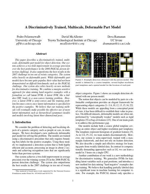
A Discriminatively Trained,Multiscale,Deformable Part ModelPedro Felzenszwalb University of Chicago pff@David McAllesterToyota Technological Institute at Chicagomcallester@Deva RamananUC Irvinedramanan@AbstractThis paper describes a discriminatively trained,multi-scale,deformable part model for object detection.Our sys-tem achieves a two-fold improvement in average precision over the best performance in the2006PASCAL person de-tection challenge.It also outperforms the best results in the 2007challenge in ten out of twenty categories.The system relies heavily on deformable parts.While deformable part models have become quite popular,their value had not been demonstrated on difficult benchmarks such as the PASCAL challenge.Our system also relies heavily on new methods for discriminative training.We combine a margin-sensitive approach for data mining hard negative examples with a formalism we call latent SVM.A latent SVM,like a hid-den CRF,leads to a non-convex training problem.How-ever,a latent SVM is semi-convex and the training prob-lem becomes convex once latent information is specified for the positive examples.We believe that our training meth-ods will eventually make possible the effective use of more latent information such as hierarchical(grammar)models and models involving latent three dimensional pose.1.IntroductionWe consider the problem of detecting and localizing ob-jects of a generic category,such as people or cars,in static images.We have developed a new multiscale deformable part model for solving this problem.The models are trained using a discriminative procedure that only requires bound-ing box labels for the positive ing these mod-els we implemented a detection system that is both highly efficient and accurate,processing an image in about2sec-onds and achieving recognition rates that are significantly better than previous systems.Our system achieves a two-fold improvement in average precision over the winning system[5]in the2006PASCAL person detection challenge.The system also outperforms the best results in the2007challenge in ten out of twenty This material is based upon work supported by the National Science Foundation under Grant No.0534820and0535174.Figure1.Example detection obtained with the person model.The model is defined by a coarse template,several higher resolution part templates and a spatial model for the location of each part. object categories.Figure1shows an example detection ob-tained with our person model.The notion that objects can be modeled by parts in a de-formable configuration provides an elegant framework for representing object categories[1–3,6,10,12,13,15,16,22]. While these models are appealing from a conceptual point of view,it has been difficult to establish their value in prac-tice.On difficult datasets,deformable models are often out-performed by“conceptually weaker”models such as rigid templates[5]or bag-of-features[23].One of our main goals is to address this performance gap.Our models include both a coarse global template cov-ering an entire object and higher resolution part templates. The templates represent histogram of gradient features[5]. As in[14,19,21],we train models discriminatively.How-ever,our system is semi-supervised,trained with a max-margin framework,and does not rely on feature detection. We also describe a simple and effective strategy for learn-ing parts from weakly-labeled data.In contrast to computa-tionally demanding approaches such as[4],we can learn a model in3hours on a single CPU.Another contribution of our work is a new methodology for discriminative training.We generalize SVMs for han-dling latent variables such as part positions,and introduce a new method for data mining“hard negative”examples dur-ing training.We believe that handling partially labeled data is a significant issue in machine learning for computer vi-sion.For example,the PASCAL dataset only specifies abounding box for each positive example of an object.We treat the position of each object part as a latent variable.We also treat the exact location of the object as a latent vari-able,requiring only that our classifier select a window that has large overlap with the labeled bounding box.A latent SVM,like a hidden CRF[19],leads to a non-convex training problem.However,unlike a hidden CRF, a latent SVM is semi-convex and the training problem be-comes convex once latent information is specified for thepositive training examples.This leads to a general coordi-nate descent algorithm for latent SVMs.System Overview Our system uses a scanning window approach.A model for an object consists of a global“root”filter and several part models.Each part model specifies a spatial model and a partfilter.The spatial model defines a set of allowed placements for a part relative to a detection window,and a deformation cost for each placement.The score of a detection window is the score of the root filter on the window plus the sum over parts,of the maxi-mum over placements of that part,of the partfilter score on the resulting subwindow minus the deformation cost.This is similar to classical part-based models[10,13].Both root and partfilters are scored by computing the dot product be-tween a set of weights and histogram of gradient(HOG) features within a window.The rootfilter is equivalent to a Dalal-Triggs model[5].The features for the partfilters are computed at twice the spatial resolution of the rootfilter. Our model is defined at afixed scale,and we detect objects by searching over an image pyramid.In training we are given a set of images annotated with bounding boxes around each instance of an object.We re-duce the detection problem to a binary classification prob-lem.Each example x is scored by a function of the form, fβ(x)=max zβ·Φ(x,z).Hereβis a vector of model pa-rameters and z are latent values(e.g.the part placements). To learn a model we define a generalization of SVMs that we call latent variable SVM(LSVM).An important prop-erty of LSVMs is that the training problem becomes convex if wefix the latent values for positive examples.This can be used in a coordinate descent algorithm.In practice we iteratively apply classical SVM training to triples( x1,z1,y1 ,..., x n,z n,y n )where z i is selected to be the best scoring latent label for x i under the model learned in the previous iteration.An initial rootfilter is generated from the bounding boxes in the PASCAL dataset. The parts are initialized from this rootfilter.2.ModelThe underlying building blocks for our models are the Histogram of Oriented Gradient(HOG)features from[5]. We represent HOG features at two different scales.Coarse features are captured by a rigid template covering anentireImage pyramidFigure2.The HOG feature pyramid and an object hypothesis de-fined in terms of a placement of the rootfilter(near the top of the pyramid)and the partfilters(near the bottom of the pyramid). detection window.Finer scale features are captured by part templates that can be moved with respect to the detection window.The spatial model for the part locations is equiv-alent to a star graph or1-fan[3]where the coarse template serves as a reference position.2.1.HOG RepresentationWe follow the construction in[5]to define a dense repre-sentation of an image at a particular resolution.The image isfirst divided into8x8non-overlapping pixel regions,or cells.For each cell we accumulate a1D histogram of gra-dient orientations over pixels in that cell.These histograms capture local shape properties but are also somewhat invari-ant to small deformations.The gradient at each pixel is discretized into one of nine orientation bins,and each pixel“votes”for the orientation of its gradient,with a strength that depends on the gradient magnitude.For color images,we compute the gradient of each color channel and pick the channel with highest gradi-ent magnitude at each pixel.Finally,the histogram of each cell is normalized with respect to the gradient energy in a neighborhood around it.We look at the four2×2blocks of cells that contain a particular cell and normalize the his-togram of the given cell with respect to the total energy in each of these blocks.This leads to a vector of length9×4 representing the local gradient information inside a cell.We define a HOG feature pyramid by computing HOG features of each level of a standard image pyramid(see Fig-ure2).Features at the top of this pyramid capture coarse gradients histogrammed over fairly large areas of the input image while features at the bottom of the pyramid capture finer gradients histogrammed over small areas.2.2.FiltersFilters are rectangular templates specifying weights for subwindows of a HOG pyramid.A w by hfilter F is a vector with w×h×9×4weights.The score of afilter is defined by taking the dot product of the weight vector and the features in a w×h subwindow of a HOG pyramid.The system in[5]uses a singlefilter to define an object model.That system detects objects from a particular class by scoring every w×h subwindow of a HOG pyramid and thresholding the scores.Let H be a HOG pyramid and p=(x,y,l)be a cell in the l-th level of the pyramid.Letφ(H,p,w,h)denote the vector obtained by concatenating the HOG features in the w×h subwindow of H with top-left corner at p.The score of F on this detection window is F·φ(H,p,w,h).Below we useφ(H,p)to denoteφ(H,p,w,h)when the dimensions are clear from context.2.3.Deformable PartsHere we consider models defined by a coarse rootfilter that covers the entire object and higher resolution partfilters covering smaller parts of the object.Figure2illustrates a placement of such a model in a HOG pyramid.The rootfil-ter location defines the detection window(the pixels inside the cells covered by thefilter).The partfilters are placed several levels down in the pyramid,so the HOG cells at that level have half the size of cells in the rootfilter level.We have found that using higher resolution features for defining partfilters is essential for obtaining high recogni-tion performance.With this approach the partfilters repre-sentfiner resolution edges that are localized to greater ac-curacy when compared to the edges represented in the root filter.For example,consider building a model for a face. The rootfilter could capture coarse resolution edges such as the face boundary while the partfilters could capture details such as eyes,nose and mouth.The model for an object with n parts is formally defined by a rootfilter F0and a set of part models(P1,...,P n) where P i=(F i,v i,s i,a i,b i).Here F i is afilter for the i-th part,v i is a two-dimensional vector specifying the center for a box of possible positions for part i relative to the root po-sition,s i gives the size of this box,while a i and b i are two-dimensional vectors specifying coefficients of a quadratic function measuring a score for each possible placement of the i-th part.Figure1illustrates a person model.A placement of a model in a HOG pyramid is given by z=(p0,...,p n),where p i=(x i,y i,l i)is the location of the rootfilter when i=0and the location of the i-th part when i>0.We assume the level of each part is such that a HOG cell at that level has half the size of a HOG cell at the root level.The score of a placement is given by the scores of eachfilter(the data term)plus a score of the placement of each part relative to the root(the spatial term), ni=0F i·φ(H,p i)+ni=1a i·(˜x i,˜y i)+b i·(˜x2i,˜y2i),(1)where(˜x i,˜y i)=((x i,y i)−2(x,y)+v i)/s i gives the lo-cation of the i-th part relative to the root location.Both˜x i and˜y i should be between−1and1.There is a large(exponential)number of placements for a model in a HOG pyramid.We use dynamic programming and distance transforms techniques[9,10]to compute the best location for the parts of a model as a function of the root location.This takes O(nk)time,where n is the number of parts in the model and k is the number of cells in the HOG pyramid.To detect objects in an image we score root locations according to the best possible placement of the parts and threshold this score.The score of a placement z can be expressed in terms of the dot product,β·ψ(H,z),between a vector of model parametersβand a vectorψ(H,z),β=(F0,...,F n,a1,b1...,a n,b n).ψ(H,z)=(φ(H,p0),φ(H,p1),...φ(H,p n),˜x1,˜y1,˜x21,˜y21,...,˜x n,˜y n,˜x2n,˜y2n,). We use this representation for learning the model parame-ters as it makes a connection between our deformable mod-els and linear classifiers.On interesting aspect of the spatial models defined here is that we allow for the coefficients(a i,b i)to be negative. This is more general than the quadratic“spring”cost that has been used in previous work.3.LearningThe PASCAL training data consists of a large set of im-ages with bounding boxes around each instance of an ob-ject.We reduce the problem of learning a deformable part model with this data to a binary classification problem.Let D=( x1,y1 ,..., x n,y n )be a set of labeled exam-ples where y i∈{−1,1}and x i specifies a HOG pyramid, H(x i),together with a range,Z(x i),of valid placements for the root and partfilters.We construct a positive exam-ple from each bounding box in the training set.For these ex-amples we define Z(x i)so the rootfilter must be placed to overlap the bounding box by at least50%.Negative exam-ples come from images that do not contain the target object. Each placement of the rootfilter in such an image yields a negative training example.Note that for the positive examples we treat both the part locations and the exact location of the rootfilter as latent variables.We have found that allowing uncertainty in the root location during training significantly improves the per-formance of the system(see Section4).tent SVMsA latent SVM is defined as follows.We assume that each example x is scored by a function of the form,fβ(x)=maxz∈Z(x)β·Φ(x,z),(2)whereβis a vector of model parameters and z is a set of latent values.For our deformable models we define Φ(x,z)=ψ(H(x),z)so thatβ·Φ(x,z)is the score of placing the model according to z.In analogy to classical SVMs we would like to trainβfrom labeled examples D=( x1,y1 ,..., x n,y n )by optimizing the following objective function,β∗(D)=argminβλ||β||2+ni=1max(0,1−y i fβ(x i)).(3)By restricting the latent domains Z(x i)to a single choice, fβbecomes linear inβ,and we obtain linear SVMs as a special case of latent tent SVMs are instances of the general class of energy-based models[18].3.2.Semi-ConvexityNote that fβ(x)as defined in(2)is a maximum of func-tions each of which is linear inβ.Hence fβ(x)is convex inβ.This implies that the hinge loss max(0,1−y i fβ(x i)) is convex inβwhen y i=−1.That is,the loss function is convex inβfor negative examples.We call this property of the loss function semi-convexity.Consider an LSVM where the latent domains Z(x i)for the positive examples are restricted to a single choice.The loss due to each positive example is now bined with the semi-convexity property,(3)becomes convex inβ.If the labels for the positive examples are notfixed we can compute a local optimum of(3)using a coordinate de-scent algorithm:1.Holdingβfixed,optimize the latent values for the pos-itive examples z i=argmax z∈Z(xi )β·Φ(x,z).2.Holding{z i}fixed for positive examples,optimizeβby solving the convex problem defined above.It can be shown that both steps always improve or maintain the value of the objective function in(3).If both steps main-tain the value we have a strong local optimum of(3),in the sense that Step1searches over an exponentially large space of latent labels for positive examples while Step2simulta-neously searches over weight vectors and an exponentially large space of latent labels for negative examples.3.3.Data Mining Hard NegativesIn object detection the vast majority of training exam-ples are negative.This makes it infeasible to consider all negative examples at a time.Instead,it is common to con-struct training data consisting of the positive instances and “hard negative”instances,where the hard negatives are data mined from the very large set of possible negative examples.Here we describe a general method for data mining ex-amples for SVMs and latent SVMs.The method iteratively solves subproblems using only hard instances.The innova-tion of our approach is a theoretical guarantee that it leads to the exact solution of the training problem defined using the complete training set.Our results require the use of a margin-sensitive definition of hard examples.The results described here apply both to classical SVMs and to the problem defined by Step2of the coordinate de-scent algorithm for latent SVMs.We omit the proofs of the theorems due to lack of space.These results are related to working set methods[17].We define the hard instances of D relative toβas,M(β,D)={ x,y ∈D|yfβ(x)≤1}.(4)That is,M(β,D)are training examples that are incorrectly classified or near the margin of the classifier defined byβ. We can show thatβ∗(D)only depends on hard instances. Theorem1.Let C be a subset of the examples in D.If M(β∗(D),D)⊆C thenβ∗(C)=β∗(D).This implies that in principle we could train a model us-ing a small set of examples.However,this set is defined in terms of the optimal modelβ∗(D).Given afixedβwe can use M(β,D)to approximate M(β∗(D),D).This suggests an iterative algorithm where we repeatedly compute a model from the hard instances de-fined by the model from the last iteration.This is further justified by the followingfixed-point theorem.Theorem2.Ifβ∗(M(β,D))=βthenβ=β∗(D).Let C be an initial“cache”of examples.In practice we can take the positive examples together with random nega-tive examples.Consider the following iterative algorithm: 1.Letβ:=β∗(C).2.Shrink C by letting C:=M(β,C).3.Grow C by adding examples from M(β,D)up to amemory limit L.Theorem3.If|C|<L after each iteration of Step2,the algorithm will converge toβ=β∗(D)infinite time.3.4.Implementation detailsMany of the ideas discussed here are only approximately implemented in our current system.In practice,when train-ing a latent SVM we iteratively apply classical SVM train-ing to triples x1,z1,y1 ,..., x n,z n,y n where z i is se-lected to be the best scoring latent label for x i under themodel trained in the previous iteration.Each of these triples leads to an example Φ(x i,z i),y i for training a linear clas-sifier.This allows us to use a highly optimized SVM pack-age(SVMLight[17]).On a single CPU,the entire training process takes3to4hours per object class in the PASCAL datasets,including initialization of the parts.Root Filter Initialization:For each category,we auto-matically select the dimensions of the rootfilter by looking at statistics of the bounding boxes in the training data.1We train an initial rootfilter F0using an SVM with no latent variables.The positive examples are constructed from the unoccluded training examples(as labeled in the PASCAL data).These examples are anisotropically scaled to the size and aspect ratio of thefilter.We use random subwindows from negative images to generate negative examples.Root Filter Update:Given the initial rootfilter trained as above,for each bounding box in the training set wefind the best-scoring placement for thefilter that significantly overlaps with the bounding box.We do this using the orig-inal,un-scaled images.We retrain F0with the new positive set and the original random negative set,iterating twice.Part Initialization:We employ a simple heuristic to ini-tialize six parts from the rootfilter trained above.First,we select an area a such that6a equals80%of the area of the rootfilter.We greedily select the rectangular region of area a from the rootfilter that has the most positive energy.We zero out the weights in this region and repeat until six parts are selected.The partfilters are initialized from the rootfil-ter values in the subwindow selected for the part,butfilled in to handle the higher spatial resolution of the part.The initial deformation costs measure the squared norm of a dis-placement with a i=(0,0)and b i=−(1,1).Model Update:To update a model we construct new training data triples.For each positive bounding box in the training data,we apply the existing detector at all positions and scales with at least a50%overlap with the given bound-ing box.Among these we select the highest scoring place-ment as the positive example corresponding to this training bounding box(Figure3).Negative examples are selected byfinding high scoring detections in images not containing the target object.We add negative examples to a cache un-til we encounterfile size limits.A new model is trained by running SVMLight on the positive and negative examples, each labeled with part placements.We update the model10 times using the cache scheme described above.In each it-eration we keep the hard instances from the previous cache and add as many new hard instances as possible within the memory limit.Toward thefinal iterations,we are able to include all hard instances,M(β,D),in the cache.1We picked a simple heuristic by cross-validating over5object classes. We set the model aspect to be the most common(mode)aspect in the data. We set the model size to be the largest size not larger than80%of thedata.Figure3.The image on the left shows the optimization of the la-tent variables for a positive example.The dotted box is the bound-ing box label provided in the PASCAL training set.The large solid box shows the placement of the detection window while the smaller solid boxes show the placements of the parts.The image on the right shows a hard-negative example.4.ResultsWe evaluated our system using the PASCAL VOC2006 and2007comp3challenge datasets and protocol.We refer to[7,8]for details,but emphasize that both challenges are widely acknowledged as difficult testbeds for object detec-tion.Each dataset contains several thousand images of real-world scenes.The datasets specify ground-truth bounding boxes for several object classes,and a detection is consid-ered correct when it overlaps more than50%with a ground-truth bounding box.One scores a system by the average precision(AP)of its precision-recall curve across a testset.Recent work in pedestrian detection has tended to report detection rates versus false positives per window,measured with cropped positive examples and negative images with-out objects of interest.These scores are tied to the reso-lution of the scanning window search and ignore effects of non-maximum suppression,making it difficult to compare different systems.We believe the PASCAL scoring method gives a more reliable measure of performance.The2007challenge has20object categories.We entered a preliminary version of our system in the official competi-tion,and obtained the best score in6categories.Our current system obtains the highest score in10categories,and the second highest score in6categories.Table1summarizes the results.Our system performs well on rigid objects such as cars and sofas as well as highly deformable objects such as per-sons and horses.We also note that our system is successful when given a large or small amount of training data.There are roughly4700positive training examples in the person category but only250in the sofa category.Figure4shows some of the models we learned.Figure5shows some ex-ample detections.We evaluated different components of our system on the longer-established2006person dataset.The top AP scoreaero bike bird boat bottle bus car cat chair cow table dog horse mbike person plant sheep sofa train tvOur rank 31211224111422112141Our score .180.411.092.098.249.349.396.110.155.165.110.062.301.337.267.140.141.156.206.336Darmstadt .301INRIA Normal .092.246.012.002.068.197.265.018.097.039.017.016.225.153.121.093.002.102.157.242INRIA Plus.136.287.041.025.077.279.294.132.106.127.067.071.335.249.092.072.011.092.242.275IRISA .281.318.026.097.119.289.227.221.175.253MPI Center .060.110.028.031.000.164.172.208.002.044.049.141.198.170.091.004.091.034.237.051MPI ESSOL.152.157.098.016.001.186.120.240.007.061.098.162.034.208.117.002.046.147.110.054Oxford .262.409.393.432.375.334TKK .186.078.043.072.002.116.184.050.028.100.086.126.186.135.061.019.036.058.067.090Table 1.PASCAL VOC 2007results.Average precision scores of our system and other systems that entered the competition [7].Empty boxes indicate that a method was not tested in the corresponding class.The best score in each class is shown in bold.Our current system ranks first in 10out of 20classes.A preliminary version of our system ranked first in 6classes in the official competition.BottleCarBicycleSofaFigure 4.Some models learned from the PASCAL VOC 2007dataset.We show the total energy in each orientation of the HOG cells in the root and part filters,with the part filters placed at the center of the allowable displacements.We also show the spatial model for each part,where bright values represent “cheap”placements,and dark values represent “expensive”placements.in the PASCAL competition was .16,obtained using a rigid template model of HOG features [5].The best previous re-sult of.19adds a segmentation-based verification step [20].Figure 6summarizes the performance of several models we trained.Our root-only model is equivalent to the model from [5]and it scores slightly higher at .18.Performance jumps to .24when the model is trained with a LSVM that selects a latent position and scale for each positive example.This suggests LSVMs are useful even for rigid templates because they allow for self-adjustment of the detection win-dow in the training examples.Adding deformable parts in-creases performance to .34AP —a factor of two above the best previous score.Finally,we trained a model with partsbut no root filter and obtained .29AP.This illustrates the advantage of using a multiscale representation.We also investigated the effect of the spatial model and allowable deformations on the 2006person dataset.Recall that s i is the allowable displacement of a part,measured in HOG cells.We trained a rigid model with high-resolution parts by setting s i to 0.This model outperforms the root-only system by .27to .24.If we increase the amount of allowable displacements without using a deformation cost,we start to approach a bag-of-features.Performance peaks at s i =1,suggesting it is useful to constrain the part dis-placements.The optimal strategy allows for larger displace-ments while using an explicit deformation cost.The follow-Figure 5.Some results from the PASCAL 2007dataset.Each row shows detections using a model for a specific class (Person,Bottle,Car,Sofa,Bicycle,Horse).The first three columns show correct detections while the last column shows false positives.Our system is able to detect objects over a wide range of scales (such as the cars)and poses (such as the horses).The system can also detect partially occluded objects such as a person behind a bush.Note how the false detections are often quite reasonable,for example detecting a bus with the car model,a bicycle sign with the bicycle model,or a dog with the horse model.In general the part filters represent meaningful object parts that are well localized in each detection such as the head in the person model.Figure6.Evaluation of our system on the PASCAL VOC2006 person dataset.Root uses only a rootfilter and no latent place-ment of the detection windows on positive examples.Root+Latent uses a rootfilter with latent placement of the detection windows. Parts+Latent is a part-based system with latent detection windows but no rootfilter.Root+Parts+Latent includes both root and part filters,and latent placement of the detection windows.ing table shows AP as a function of freely allowable defor-mation in thefirst three columns.The last column gives the performance when using a quadratic deformation cost and an allowable displacement of2HOG cells.s i01232+quadratic costAP.27.33.31.31.345.DiscussionWe introduced a general framework for training SVMs with latent structure.We used it to build a recognition sys-tem based on multiscale,deformable models.Experimental results on difficult benchmark data suggests our system is the current state-of-the-art in object detection.LSVMs allow for exploration of additional latent struc-ture for recognition.One can consider deeper part hierar-chies(parts with parts),mixture models(frontal vs.side cars),and three-dimensional pose.We would like to train and detect multiple classes together using a shared vocab-ulary of parts(perhaps visual words).We also plan to use A*search[11]to efficiently search over latent parameters during detection.References[1]Y.Amit and A.Trouve.POP:Patchwork of parts models forobject recognition.IJCV,75(2):267–282,November2007.[2]M.Burl,M.Weber,and P.Perona.A probabilistic approachto object recognition using local photometry and global ge-ometry.In ECCV,pages II:628–641,1998.[3] D.Crandall,P.Felzenszwalb,and D.Huttenlocher.Spatialpriors for part-based recognition using statistical models.In CVPR,pages10–17,2005.[4] D.Crandall and D.Huttenlocher.Weakly supervised learn-ing of part-based spatial models for visual object recognition.In ECCV,pages I:16–29,2006.[5]N.Dalal and B.Triggs.Histograms of oriented gradients forhuman detection.In CVPR,pages I:886–893,2005.[6] B.Epshtein and S.Ullman.Semantic hierarchies for recog-nizing objects and parts.In CVPR,2007.[7]M.Everingham,L.Van Gool,C.K.I.Williams,J.Winn,and A.Zisserman.The PASCAL Visual Object Classes Challenge2007(VOC2007)Results./challenges/VOC/voc2007/workshop.[8]M.Everingham, A.Zisserman, C.K.I.Williams,andL.Van Gool.The PASCAL Visual Object Classes Challenge2006(VOC2006)Results./challenges/VOC/voc2006/results.pdf.[9]P.Felzenszwalb and D.Huttenlocher.Distance transformsof sampled functions.Cornell Computing and Information Science Technical Report TR2004-1963,September2004.[10]P.Felzenszwalb and D.Huttenlocher.Pictorial structures forobject recognition.IJCV,61(1),2005.[11]P.Felzenszwalb and D.McAllester.The generalized A*ar-chitecture.JAIR,29:153–190,2007.[12]R.Fergus,P.Perona,and A.Zisserman.Object class recog-nition by unsupervised scale-invariant learning.In CVPR, 2003.[13]M.Fischler and R.Elschlager.The representation andmatching of pictorial structures.IEEE Transactions on Com-puter,22(1):67–92,January1973.[14] A.Holub and P.Perona.A discriminative framework formodelling object classes.In CVPR,pages I:664–671,2005.[15]S.Ioffe and D.Forsyth.Probabilistic methods forfindingpeople.IJCV,43(1):45–68,June2001.[16]Y.Jin and S.Geman.Context and hierarchy in a probabilisticimage model.In CVPR,pages II:2145–2152,2006.[17]T.Joachims.Making large-scale svm learning practical.InB.Sch¨o lkopf,C.Burges,and A.Smola,editors,Advances inKernel Methods-Support Vector Learning.MIT Press,1999.[18]Y.LeCun,S.Chopra,R.Hadsell,R.Marc’Aurelio,andF.Huang.A tutorial on energy-based learning.InG.Bakir,T.Hofman,B.Sch¨o lkopf,A.Smola,and B.Taskar,editors, Predicting Structured Data.MIT Press,2006.[19] A.Quattoni,S.Wang,L.Morency,M.Collins,and T.Dar-rell.Hidden conditional randomfields.PAMI,29(10):1848–1852,October2007.[20] ing segmentation to verify object hypothe-ses.In CVPR,pages1–8,2007.[21] D.Ramanan and C.Sminchisescu.Training deformablemodels for localization.In CVPR,pages I:206–213,2006.[22]H.Schneiderman and T.Kanade.Object detection using thestatistics of parts.IJCV,56(3):151–177,February2004. [23]J.Zhang,M.Marszalek,zebnik,and C.Schmid.Localfeatures and kernels for classification of texture and object categories:A comprehensive study.IJCV,73(2):213–238, June2007.。
机器学习与人工智能领域中常用的英语词汇
机器学习与人工智能领域中常用的英语词汇1.General Concepts (基础概念)•Artificial Intelligence (AI) - 人工智能1)Artificial Intelligence (AI) - 人工智能2)Machine Learning (ML) - 机器学习3)Deep Learning (DL) - 深度学习4)Neural Network - 神经网络5)Natural Language Processing (NLP) - 自然语言处理6)Computer Vision - 计算机视觉7)Robotics - 机器人技术8)Speech Recognition - 语音识别9)Expert Systems - 专家系统10)Knowledge Representation - 知识表示11)Pattern Recognition - 模式识别12)Cognitive Computing - 认知计算13)Autonomous Systems - 自主系统14)Human-Machine Interaction - 人机交互15)Intelligent Agents - 智能代理16)Machine Translation - 机器翻译17)Swarm Intelligence - 群体智能18)Genetic Algorithms - 遗传算法19)Fuzzy Logic - 模糊逻辑20)Reinforcement Learning - 强化学习•Machine Learning (ML) - 机器学习1)Machine Learning (ML) - 机器学习2)Artificial Neural Network - 人工神经网络3)Deep Learning - 深度学习4)Supervised Learning - 有监督学习5)Unsupervised Learning - 无监督学习6)Reinforcement Learning - 强化学习7)Semi-Supervised Learning - 半监督学习8)Training Data - 训练数据9)Test Data - 测试数据10)Validation Data - 验证数据11)Feature - 特征12)Label - 标签13)Model - 模型14)Algorithm - 算法15)Regression - 回归16)Classification - 分类17)Clustering - 聚类18)Dimensionality Reduction - 降维19)Overfitting - 过拟合20)Underfitting - 欠拟合•Deep Learning (DL) - 深度学习1)Deep Learning - 深度学习2)Neural Network - 神经网络3)Artificial Neural Network (ANN) - 人工神经网络4)Convolutional Neural Network (CNN) - 卷积神经网络5)Recurrent Neural Network (RNN) - 循环神经网络6)Long Short-Term Memory (LSTM) - 长短期记忆网络7)Gated Recurrent Unit (GRU) - 门控循环单元8)Autoencoder - 自编码器9)Generative Adversarial Network (GAN) - 生成对抗网络10)Transfer Learning - 迁移学习11)Pre-trained Model - 预训练模型12)Fine-tuning - 微调13)Feature Extraction - 特征提取14)Activation Function - 激活函数15)Loss Function - 损失函数16)Gradient Descent - 梯度下降17)Backpropagation - 反向传播18)Epoch - 训练周期19)Batch Size - 批量大小20)Dropout - 丢弃法•Neural Network - 神经网络1)Neural Network - 神经网络2)Artificial Neural Network (ANN) - 人工神经网络3)Deep Neural Network (DNN) - 深度神经网络4)Convolutional Neural Network (CNN) - 卷积神经网络5)Recurrent Neural Network (RNN) - 循环神经网络6)Long Short-Term Memory (LSTM) - 长短期记忆网络7)Gated Recurrent Unit (GRU) - 门控循环单元8)Feedforward Neural Network - 前馈神经网络9)Multi-layer Perceptron (MLP) - 多层感知器10)Radial Basis Function Network (RBFN) - 径向基函数网络11)Hopfield Network - 霍普菲尔德网络12)Boltzmann Machine - 玻尔兹曼机13)Autoencoder - 自编码器14)Spiking Neural Network (SNN) - 脉冲神经网络15)Self-organizing Map (SOM) - 自组织映射16)Restricted Boltzmann Machine (RBM) - 受限玻尔兹曼机17)Hebbian Learning - 海比安学习18)Competitive Learning - 竞争学习19)Neuroevolutionary - 神经进化20)Neuron - 神经元•Algorithm - 算法1)Algorithm - 算法2)Supervised Learning Algorithm - 有监督学习算法3)Unsupervised Learning Algorithm - 无监督学习算法4)Reinforcement Learning Algorithm - 强化学习算法5)Classification Algorithm - 分类算法6)Regression Algorithm - 回归算法7)Clustering Algorithm - 聚类算法8)Dimensionality Reduction Algorithm - 降维算法9)Decision Tree Algorithm - 决策树算法10)Random Forest Algorithm - 随机森林算法11)Support Vector Machine (SVM) Algorithm - 支持向量机算法12)K-Nearest Neighbors (KNN) Algorithm - K近邻算法13)Naive Bayes Algorithm - 朴素贝叶斯算法14)Gradient Descent Algorithm - 梯度下降算法15)Genetic Algorithm - 遗传算法16)Neural Network Algorithm - 神经网络算法17)Deep Learning Algorithm - 深度学习算法18)Ensemble Learning Algorithm - 集成学习算法19)Reinforcement Learning Algorithm - 强化学习算法20)Metaheuristic Algorithm - 元启发式算法•Model - 模型1)Model - 模型2)Machine Learning Model - 机器学习模型3)Artificial Intelligence Model - 人工智能模型4)Predictive Model - 预测模型5)Classification Model - 分类模型6)Regression Model - 回归模型7)Generative Model - 生成模型8)Discriminative Model - 判别模型9)Probabilistic Model - 概率模型10)Statistical Model - 统计模型11)Neural Network Model - 神经网络模型12)Deep Learning Model - 深度学习模型13)Ensemble Model - 集成模型14)Reinforcement Learning Model - 强化学习模型15)Support Vector Machine (SVM) Model - 支持向量机模型16)Decision Tree Model - 决策树模型17)Random Forest Model - 随机森林模型18)Naive Bayes Model - 朴素贝叶斯模型19)Autoencoder Model - 自编码器模型20)Convolutional Neural Network (CNN) Model - 卷积神经网络模型•Dataset - 数据集1)Dataset - 数据集2)Training Dataset - 训练数据集3)Test Dataset - 测试数据集4)Validation Dataset - 验证数据集5)Balanced Dataset - 平衡数据集6)Imbalanced Dataset - 不平衡数据集7)Synthetic Dataset - 合成数据集8)Benchmark Dataset - 基准数据集9)Open Dataset - 开放数据集10)Labeled Dataset - 标记数据集11)Unlabeled Dataset - 未标记数据集12)Semi-Supervised Dataset - 半监督数据集13)Multiclass Dataset - 多分类数据集14)Feature Set - 特征集15)Data Augmentation - 数据增强16)Data Preprocessing - 数据预处理17)Missing Data - 缺失数据18)Outlier Detection - 异常值检测19)Data Imputation - 数据插补20)Metadata - 元数据•Training - 训练1)Training - 训练2)Training Data - 训练数据3)Training Phase - 训练阶段4)Training Set - 训练集5)Training Examples - 训练样本6)Training Instance - 训练实例7)Training Algorithm - 训练算法8)Training Model - 训练模型9)Training Process - 训练过程10)Training Loss - 训练损失11)Training Epoch - 训练周期12)Training Batch - 训练批次13)Online Training - 在线训练14)Offline Training - 离线训练15)Continuous Training - 连续训练16)Transfer Learning - 迁移学习17)Fine-Tuning - 微调18)Curriculum Learning - 课程学习19)Self-Supervised Learning - 自监督学习20)Active Learning - 主动学习•Testing - 测试1)Testing - 测试2)Test Data - 测试数据3)Test Set - 测试集4)Test Examples - 测试样本5)Test Instance - 测试实例6)Test Phase - 测试阶段7)Test Accuracy - 测试准确率8)Test Loss - 测试损失9)Test Error - 测试错误10)Test Metrics - 测试指标11)Test Suite - 测试套件12)Test Case - 测试用例13)Test Coverage - 测试覆盖率14)Cross-Validation - 交叉验证15)Holdout Validation - 留出验证16)K-Fold Cross-Validation - K折交叉验证17)Stratified Cross-Validation - 分层交叉验证18)Test Driven Development (TDD) - 测试驱动开发19)A/B Testing - A/B 测试20)Model Evaluation - 模型评估•Validation - 验证1)Validation - 验证2)Validation Data - 验证数据3)Validation Set - 验证集4)Validation Examples - 验证样本5)Validation Instance - 验证实例6)Validation Phase - 验证阶段7)Validation Accuracy - 验证准确率8)Validation Loss - 验证损失9)Validation Error - 验证错误10)Validation Metrics - 验证指标11)Cross-Validation - 交叉验证12)Holdout Validation - 留出验证13)K-Fold Cross-Validation - K折交叉验证14)Stratified Cross-Validation - 分层交叉验证15)Leave-One-Out Cross-Validation - 留一法交叉验证16)Validation Curve - 验证曲线17)Hyperparameter Validation - 超参数验证18)Model Validation - 模型验证19)Early Stopping - 提前停止20)Validation Strategy - 验证策略•Supervised Learning - 有监督学习1)Supervised Learning - 有监督学习2)Label - 标签3)Feature - 特征4)Target - 目标5)Training Labels - 训练标签6)Training Features - 训练特征7)Training Targets - 训练目标8)Training Examples - 训练样本9)Training Instance - 训练实例10)Regression - 回归11)Classification - 分类12)Predictor - 预测器13)Regression Model - 回归模型14)Classifier - 分类器15)Decision Tree - 决策树16)Support Vector Machine (SVM) - 支持向量机17)Neural Network - 神经网络18)Feature Engineering - 特征工程19)Model Evaluation - 模型评估20)Overfitting - 过拟合21)Underfitting - 欠拟合22)Bias-Variance Tradeoff - 偏差-方差权衡•Unsupervised Learning - 无监督学习1)Unsupervised Learning - 无监督学习2)Clustering - 聚类3)Dimensionality Reduction - 降维4)Anomaly Detection - 异常检测5)Association Rule Learning - 关联规则学习6)Feature Extraction - 特征提取7)Feature Selection - 特征选择8)K-Means - K均值9)Hierarchical Clustering - 层次聚类10)Density-Based Clustering - 基于密度的聚类11)Principal Component Analysis (PCA) - 主成分分析12)Independent Component Analysis (ICA) - 独立成分分析13)T-distributed Stochastic Neighbor Embedding (t-SNE) - t分布随机邻居嵌入14)Gaussian Mixture Model (GMM) - 高斯混合模型15)Self-Organizing Maps (SOM) - 自组织映射16)Autoencoder - 自动编码器17)Latent Variable - 潜变量18)Data Preprocessing - 数据预处理19)Outlier Detection - 异常值检测20)Clustering Algorithm - 聚类算法•Reinforcement Learning - 强化学习1)Reinforcement Learning - 强化学习2)Agent - 代理3)Environment - 环境4)State - 状态5)Action - 动作6)Reward - 奖励7)Policy - 策略8)Value Function - 值函数9)Q-Learning - Q学习10)Deep Q-Network (DQN) - 深度Q网络11)Policy Gradient - 策略梯度12)Actor-Critic - 演员-评论家13)Exploration - 探索14)Exploitation - 开发15)Temporal Difference (TD) - 时间差分16)Markov Decision Process (MDP) - 马尔可夫决策过程17)State-Action-Reward-State-Action (SARSA) - 状态-动作-奖励-状态-动作18)Policy Iteration - 策略迭代19)Value Iteration - 值迭代20)Monte Carlo Methods - 蒙特卡洛方法•Semi-Supervised Learning - 半监督学习1)Semi-Supervised Learning - 半监督学习2)Labeled Data - 有标签数据3)Unlabeled Data - 无标签数据4)Label Propagation - 标签传播5)Self-Training - 自训练6)Co-Training - 协同训练7)Transudative Learning - 传导学习8)Inductive Learning - 归纳学习9)Manifold Regularization - 流形正则化10)Graph-based Methods - 基于图的方法11)Cluster Assumption - 聚类假设12)Low-Density Separation - 低密度分离13)Semi-Supervised Support Vector Machines (S3VM) - 半监督支持向量机14)Expectation-Maximization (EM) - 期望最大化15)Co-EM - 协同期望最大化16)Entropy-Regularized EM - 熵正则化EM17)Mean Teacher - 平均教师18)Virtual Adversarial Training - 虚拟对抗训练19)Tri-training - 三重训练20)Mix Match - 混合匹配•Feature - 特征1)Feature - 特征2)Feature Engineering - 特征工程3)Feature Extraction - 特征提取4)Feature Selection - 特征选择5)Input Features - 输入特征6)Output Features - 输出特征7)Feature Vector - 特征向量8)Feature Space - 特征空间9)Feature Representation - 特征表示10)Feature Transformation - 特征转换11)Feature Importance - 特征重要性12)Feature Scaling - 特征缩放13)Feature Normalization - 特征归一化14)Feature Encoding - 特征编码15)Feature Fusion - 特征融合16)Feature Dimensionality Reduction - 特征维度减少17)Continuous Feature - 连续特征18)Categorical Feature - 分类特征19)Nominal Feature - 名义特征20)Ordinal Feature - 有序特征•Label - 标签1)Label - 标签2)Labeling - 标注3)Ground Truth - 地面真值4)Class Label - 类别标签5)Target Variable - 目标变量6)Labeling Scheme - 标注方案7)Multi-class Labeling - 多类别标注8)Binary Labeling - 二分类标注9)Label Noise - 标签噪声10)Labeling Error - 标注错误11)Label Propagation - 标签传播12)Unlabeled Data - 无标签数据13)Labeled Data - 有标签数据14)Semi-supervised Learning - 半监督学习15)Active Learning - 主动学习16)Weakly Supervised Learning - 弱监督学习17)Noisy Label Learning - 噪声标签学习18)Self-training - 自训练19)Crowdsourcing Labeling - 众包标注20)Label Smoothing - 标签平滑化•Prediction - 预测1)Prediction - 预测2)Forecasting - 预测3)Regression - 回归4)Classification - 分类5)Time Series Prediction - 时间序列预测6)Forecast Accuracy - 预测准确性7)Predictive Modeling - 预测建模8)Predictive Analytics - 预测分析9)Forecasting Method - 预测方法10)Predictive Performance - 预测性能11)Predictive Power - 预测能力12)Prediction Error - 预测误差13)Prediction Interval - 预测区间14)Prediction Model - 预测模型15)Predictive Uncertainty - 预测不确定性16)Forecast Horizon - 预测时间跨度17)Predictive Maintenance - 预测性维护18)Predictive Policing - 预测式警务19)Predictive Healthcare - 预测性医疗20)Predictive Maintenance - 预测性维护•Classification - 分类1)Classification - 分类2)Classifier - 分类器3)Class - 类别4)Classify - 对数据进行分类5)Class Label - 类别标签6)Binary Classification - 二元分类7)Multiclass Classification - 多类分类8)Class Probability - 类别概率9)Decision Boundary - 决策边界10)Decision Tree - 决策树11)Support Vector Machine (SVM) - 支持向量机12)K-Nearest Neighbors (KNN) - K最近邻算法13)Naive Bayes - 朴素贝叶斯14)Logistic Regression - 逻辑回归15)Random Forest - 随机森林16)Neural Network - 神经网络17)SoftMax Function - SoftMax函数18)One-vs-All (One-vs-Rest) - 一对多(一对剩余)19)Ensemble Learning - 集成学习20)Confusion Matrix - 混淆矩阵•Regression - 回归1)Regression Analysis - 回归分析2)Linear Regression - 线性回归3)Multiple Regression - 多元回归4)Polynomial Regression - 多项式回归5)Logistic Regression - 逻辑回归6)Ridge Regression - 岭回归7)Lasso Regression - Lasso回归8)Elastic Net Regression - 弹性网络回归9)Regression Coefficients - 回归系数10)Residuals - 残差11)Ordinary Least Squares (OLS) - 普通最小二乘法12)Ridge Regression Coefficient - 岭回归系数13)Lasso Regression Coefficient - Lasso回归系数14)Elastic Net Regression Coefficient - 弹性网络回归系数15)Regression Line - 回归线16)Prediction Error - 预测误差17)Regression Model - 回归模型18)Nonlinear Regression - 非线性回归19)Generalized Linear Models (GLM) - 广义线性模型20)Coefficient of Determination (R-squared) - 决定系数21)F-test - F检验22)Homoscedasticity - 同方差性23)Heteroscedasticity - 异方差性24)Autocorrelation - 自相关25)Multicollinearity - 多重共线性26)Outliers - 异常值27)Cross-validation - 交叉验证28)Feature Selection - 特征选择29)Feature Engineering - 特征工程30)Regularization - 正则化2.Neural Networks and Deep Learning (神经网络与深度学习)•Convolutional Neural Network (CNN) - 卷积神经网络1)Convolutional Neural Network (CNN) - 卷积神经网络2)Convolution Layer - 卷积层3)Feature Map - 特征图4)Convolution Operation - 卷积操作5)Stride - 步幅6)Padding - 填充7)Pooling Layer - 池化层8)Max Pooling - 最大池化9)Average Pooling - 平均池化10)Fully Connected Layer - 全连接层11)Activation Function - 激活函数12)Rectified Linear Unit (ReLU) - 线性修正单元13)Dropout - 随机失活14)Batch Normalization - 批量归一化15)Transfer Learning - 迁移学习16)Fine-Tuning - 微调17)Image Classification - 图像分类18)Object Detection - 物体检测19)Semantic Segmentation - 语义分割20)Instance Segmentation - 实例分割21)Generative Adversarial Network (GAN) - 生成对抗网络22)Image Generation - 图像生成23)Style Transfer - 风格迁移24)Convolutional Autoencoder - 卷积自编码器25)Recurrent Neural Network (RNN) - 循环神经网络•Recurrent Neural Network (RNN) - 循环神经网络1)Recurrent Neural Network (RNN) - 循环神经网络2)Long Short-Term Memory (LSTM) - 长短期记忆网络3)Gated Recurrent Unit (GRU) - 门控循环单元4)Sequence Modeling - 序列建模5)Time Series Prediction - 时间序列预测6)Natural Language Processing (NLP) - 自然语言处理7)Text Generation - 文本生成8)Sentiment Analysis - 情感分析9)Named Entity Recognition (NER) - 命名实体识别10)Part-of-Speech Tagging (POS Tagging) - 词性标注11)Sequence-to-Sequence (Seq2Seq) - 序列到序列12)Attention Mechanism - 注意力机制13)Encoder-Decoder Architecture - 编码器-解码器架构14)Bidirectional RNN - 双向循环神经网络15)Teacher Forcing - 强制教师法16)Backpropagation Through Time (BPTT) - 通过时间的反向传播17)Vanishing Gradient Problem - 梯度消失问题18)Exploding Gradient Problem - 梯度爆炸问题19)Language Modeling - 语言建模20)Speech Recognition - 语音识别•Long Short-Term Memory (LSTM) - 长短期记忆网络1)Long Short-Term Memory (LSTM) - 长短期记忆网络2)Cell State - 细胞状态3)Hidden State - 隐藏状态4)Forget Gate - 遗忘门5)Input Gate - 输入门6)Output Gate - 输出门7)Peephole Connections - 窥视孔连接8)Gated Recurrent Unit (GRU) - 门控循环单元9)Vanishing Gradient Problem - 梯度消失问题10)Exploding Gradient Problem - 梯度爆炸问题11)Sequence Modeling - 序列建模12)Time Series Prediction - 时间序列预测13)Natural Language Processing (NLP) - 自然语言处理14)Text Generation - 文本生成15)Sentiment Analysis - 情感分析16)Named Entity Recognition (NER) - 命名实体识别17)Part-of-Speech Tagging (POS Tagging) - 词性标注18)Attention Mechanism - 注意力机制19)Encoder-Decoder Architecture - 编码器-解码器架构20)Bidirectional LSTM - 双向长短期记忆网络•Attention Mechanism - 注意力机制1)Attention Mechanism - 注意力机制2)Self-Attention - 自注意力3)Multi-Head Attention - 多头注意力4)Transformer - 变换器5)Query - 查询6)Key - 键7)Value - 值8)Query-Value Attention - 查询-值注意力9)Dot-Product Attention - 点积注意力10)Scaled Dot-Product Attention - 缩放点积注意力11)Additive Attention - 加性注意力12)Context Vector - 上下文向量13)Attention Score - 注意力分数14)SoftMax Function - SoftMax函数15)Attention Weight - 注意力权重16)Global Attention - 全局注意力17)Local Attention - 局部注意力18)Positional Encoding - 位置编码19)Encoder-Decoder Attention - 编码器-解码器注意力20)Cross-Modal Attention - 跨模态注意力•Generative Adversarial Network (GAN) - 生成对抗网络1)Generative Adversarial Network (GAN) - 生成对抗网络2)Generator - 生成器3)Discriminator - 判别器4)Adversarial Training - 对抗训练5)Minimax Game - 极小极大博弈6)Nash Equilibrium - 纳什均衡7)Mode Collapse - 模式崩溃8)Training Stability - 训练稳定性9)Loss Function - 损失函数10)Discriminative Loss - 判别损失11)Generative Loss - 生成损失12)Wasserstein GAN (WGAN) - Wasserstein GAN(WGAN)13)Deep Convolutional GAN (DCGAN) - 深度卷积生成对抗网络(DCGAN)14)Conditional GAN (c GAN) - 条件生成对抗网络(c GAN)15)Style GAN - 风格生成对抗网络16)Cycle GAN - 循环生成对抗网络17)Progressive Growing GAN (PGGAN) - 渐进式增长生成对抗网络(PGGAN)18)Self-Attention GAN (SAGAN) - 自注意力生成对抗网络(SAGAN)19)Big GAN - 大规模生成对抗网络20)Adversarial Examples - 对抗样本•Encoder-Decoder - 编码器-解码器1)Encoder-Decoder Architecture - 编码器-解码器架构2)Encoder - 编码器3)Decoder - 解码器4)Sequence-to-Sequence Model (Seq2Seq) - 序列到序列模型5)State Vector - 状态向量6)Context Vector - 上下文向量7)Hidden State - 隐藏状态8)Attention Mechanism - 注意力机制9)Teacher Forcing - 强制教师法10)Beam Search - 束搜索11)Recurrent Neural Network (RNN) - 循环神经网络12)Long Short-Term Memory (LSTM) - 长短期记忆网络13)Gated Recurrent Unit (GRU) - 门控循环单元14)Bidirectional Encoder - 双向编码器15)Greedy Decoding - 贪婪解码16)Masking - 遮盖17)Dropout - 随机失活18)Embedding Layer - 嵌入层19)Cross-Entropy Loss - 交叉熵损失20)Tokenization - 令牌化•Transfer Learning - 迁移学习1)Transfer Learning - 迁移学习2)Source Domain - 源领域3)Target Domain - 目标领域4)Fine-Tuning - 微调5)Domain Adaptation - 领域自适应6)Pre-Trained Model - 预训练模型7)Feature Extraction - 特征提取8)Knowledge Transfer - 知识迁移9)Unsupervised Domain Adaptation - 无监督领域自适应10)Semi-Supervised Domain Adaptation - 半监督领域自适应11)Multi-Task Learning - 多任务学习12)Data Augmentation - 数据增强13)Task Transfer - 任务迁移14)Model Agnostic Meta-Learning (MAML) - 与模型无关的元学习(MAML)15)One-Shot Learning - 单样本学习16)Zero-Shot Learning - 零样本学习17)Few-Shot Learning - 少样本学习18)Knowledge Distillation - 知识蒸馏19)Representation Learning - 表征学习20)Adversarial Transfer Learning - 对抗迁移学习•Pre-trained Models - 预训练模型1)Pre-trained Model - 预训练模型2)Transfer Learning - 迁移学习3)Fine-Tuning - 微调4)Knowledge Transfer - 知识迁移5)Domain Adaptation - 领域自适应6)Feature Extraction - 特征提取7)Representation Learning - 表征学习8)Language Model - 语言模型9)Bidirectional Encoder Representations from Transformers (BERT) - 双向编码器结构转换器10)Generative Pre-trained Transformer (GPT) - 生成式预训练转换器11)Transformer-based Models - 基于转换器的模型12)Masked Language Model (MLM) - 掩蔽语言模型13)Cloze Task - 填空任务14)Tokenization - 令牌化15)Word Embeddings - 词嵌入16)Sentence Embeddings - 句子嵌入17)Contextual Embeddings - 上下文嵌入18)Self-Supervised Learning - 自监督学习19)Large-Scale Pre-trained Models - 大规模预训练模型•Loss Function - 损失函数1)Loss Function - 损失函数2)Mean Squared Error (MSE) - 均方误差3)Mean Absolute Error (MAE) - 平均绝对误差4)Cross-Entropy Loss - 交叉熵损失5)Binary Cross-Entropy Loss - 二元交叉熵损失6)Categorical Cross-Entropy Loss - 分类交叉熵损失7)Hinge Loss - 合页损失8)Huber Loss - Huber损失9)Wasserstein Distance - Wasserstein距离10)Triplet Loss - 三元组损失11)Contrastive Loss - 对比损失12)Dice Loss - Dice损失13)Focal Loss - 焦点损失14)GAN Loss - GAN损失15)Adversarial Loss - 对抗损失16)L1 Loss - L1损失17)L2 Loss - L2损失18)Huber Loss - Huber损失19)Quantile Loss - 分位数损失•Activation Function - 激活函数1)Activation Function - 激活函数2)Sigmoid Function - Sigmoid函数3)Hyperbolic Tangent Function (Tanh) - 双曲正切函数4)Rectified Linear Unit (Re LU) - 矩形线性单元5)Parametric Re LU (P Re LU) - 参数化Re LU6)Exponential Linear Unit (ELU) - 指数线性单元7)Swish Function - Swish函数8)Softplus Function - Soft plus函数9)Softmax Function - SoftMax函数10)Hard Tanh Function - 硬双曲正切函数11)Softsign Function - Softsign函数12)GELU (Gaussian Error Linear Unit) - GELU(高斯误差线性单元)13)Mish Function - Mish函数14)CELU (Continuous Exponential Linear Unit) - CELU(连续指数线性单元)15)Bent Identity Function - 弯曲恒等函数16)Gaussian Error Linear Units (GELUs) - 高斯误差线性单元17)Adaptive Piecewise Linear (APL) - 自适应分段线性函数18)Radial Basis Function (RBF) - 径向基函数•Backpropagation - 反向传播1)Backpropagation - 反向传播2)Gradient Descent - 梯度下降3)Partial Derivative - 偏导数4)Chain Rule - 链式法则5)Forward Pass - 前向传播6)Backward Pass - 反向传播7)Computational Graph - 计算图8)Neural Network - 神经网络9)Loss Function - 损失函数10)Gradient Calculation - 梯度计算11)Weight Update - 权重更新12)Activation Function - 激活函数13)Optimizer - 优化器14)Learning Rate - 学习率15)Mini-Batch Gradient Descent - 小批量梯度下降16)Stochastic Gradient Descent (SGD) - 随机梯度下降17)Batch Gradient Descent - 批量梯度下降18)Momentum - 动量19)Adam Optimizer - Adam优化器20)Learning Rate Decay - 学习率衰减•Gradient Descent - 梯度下降1)Gradient Descent - 梯度下降2)Stochastic Gradient Descent (SGD) - 随机梯度下降3)Mini-Batch Gradient Descent - 小批量梯度下降4)Batch Gradient Descent - 批量梯度下降5)Learning Rate - 学习率6)Momentum - 动量7)Adaptive Moment Estimation (Adam) - 自适应矩估计8)RMSprop - 均方根传播9)Learning Rate Schedule - 学习率调度10)Convergence - 收敛11)Divergence - 发散12)Adagrad - 自适应学习速率方法13)Adadelta - 自适应增量学习率方法14)Adamax - 自适应矩估计的扩展版本15)Nadam - Nesterov Accelerated Adaptive Moment Estimation16)Learning Rate Decay - 学习率衰减17)Step Size - 步长18)Conjugate Gradient Descent - 共轭梯度下降19)Line Search - 线搜索20)Newton's Method - 牛顿法•Learning Rate - 学习率1)Learning Rate - 学习率2)Adaptive Learning Rate - 自适应学习率3)Learning Rate Decay - 学习率衰减4)Initial Learning Rate - 初始学习率5)Step Size - 步长6)Momentum - 动量7)Exponential Decay - 指数衰减8)Annealing - 退火9)Cyclical Learning Rate - 循环学习率10)Learning Rate Schedule - 学习率调度11)Warm-up - 预热12)Learning Rate Policy - 学习率策略13)Learning Rate Annealing - 学习率退火14)Cosine Annealing - 余弦退火15)Gradient Clipping - 梯度裁剪16)Adapting Learning Rate - 适应学习率17)Learning Rate Multiplier - 学习率倍增器18)Learning Rate Reduction - 学习率降低19)Learning Rate Update - 学习率更新20)Scheduled Learning Rate - 定期学习率•Batch Size - 批量大小1)Batch Size - 批量大小2)Mini-Batch - 小批量3)Batch Gradient Descent - 批量梯度下降4)Stochastic Gradient Descent (SGD) - 随机梯度下降5)Mini-Batch Gradient Descent - 小批量梯度下降6)Online Learning - 在线学习7)Full-Batch - 全批量8)Data Batch - 数据批次9)Training Batch - 训练批次10)Batch Normalization - 批量归一化11)Batch-wise Optimization - 批量优化12)Batch Processing - 批量处理13)Batch Sampling - 批量采样14)Adaptive Batch Size - 自适应批量大小15)Batch Splitting - 批量分割16)Dynamic Batch Size - 动态批量大小17)Fixed Batch Size - 固定批量大小18)Batch-wise Inference - 批量推理19)Batch-wise Training - 批量训练20)Batch Shuffling - 批量洗牌•Epoch - 训练周期1)Training Epoch - 训练周期2)Epoch Size - 周期大小3)Early Stopping - 提前停止4)Validation Set - 验证集5)Training Set - 训练集6)Test Set - 测试集7)Overfitting - 过拟合8)Underfitting - 欠拟合9)Model Evaluation - 模型评估10)Model Selection - 模型选择11)Hyperparameter Tuning - 超参数调优12)Cross-Validation - 交叉验证13)K-fold Cross-Validation - K折交叉验证14)Stratified Cross-Validation - 分层交叉验证15)Leave-One-Out Cross-Validation (LOOCV) - 留一法交叉验证16)Grid Search - 网格搜索17)Random Search - 随机搜索18)Model Complexity - 模型复杂度19)Learning Curve - 学习曲线20)Convergence - 收敛3.Machine Learning Techniques and Algorithms (机器学习技术与算法)•Decision Tree - 决策树1)Decision Tree - 决策树2)Node - 节点3)Root Node - 根节点4)Leaf Node - 叶节点5)Internal Node - 内部节点6)Splitting Criterion - 分裂准则7)Gini Impurity - 基尼不纯度8)Entropy - 熵9)Information Gain - 信息增益10)Gain Ratio - 增益率11)Pruning - 剪枝12)Recursive Partitioning - 递归分割13)CART (Classification and Regression Trees) - 分类回归树14)ID3 (Iterative Dichotomiser 3) - 迭代二叉树315)C4.5 (successor of ID3) - C4.5(ID3的后继者)16)C5.0 (successor of C4.5) - C5.0(C4.5的后继者)17)Split Point - 分裂点18)Decision Boundary - 决策边界19)Pruned Tree - 剪枝后的树20)Decision Tree Ensemble - 决策树集成•Random Forest - 随机森林1)Random Forest - 随机森林2)Ensemble Learning - 集成学习3)Bootstrap Sampling - 自助采样4)Bagging (Bootstrap Aggregating) - 装袋法5)Out-of-Bag (OOB) Error - 袋外误差6)Feature Subset - 特征子集7)Decision Tree - 决策树8)Base Estimator - 基础估计器9)Tree Depth - 树深度10)Randomization - 随机化11)Majority Voting - 多数投票12)Feature Importance - 特征重要性13)OOB Score - 袋外得分14)Forest Size - 森林大小15)Max Features - 最大特征数16)Min Samples Split - 最小分裂样本数17)Min Samples Leaf - 最小叶节点样本数18)Gini Impurity - 基尼不纯度19)Entropy - 熵20)Variable Importance - 变量重要性•Support Vector Machine (SVM) - 支持向量机1)Support Vector Machine (SVM) - 支持向量机2)Hyperplane - 超平面3)Kernel Trick - 核技巧4)Kernel Function - 核函数5)Margin - 间隔6)Support Vectors - 支持向量7)Decision Boundary - 决策边界8)Maximum Margin Classifier - 最大间隔分类器9)Soft Margin Classifier - 软间隔分类器10) C Parameter - C参数11)Radial Basis Function (RBF) Kernel - 径向基函数核12)Polynomial Kernel - 多项式核13)Linear Kernel - 线性核14)Quadratic Kernel - 二次核15)Gaussian Kernel - 高斯核16)Regularization - 正则化17)Dual Problem - 对偶问题18)Primal Problem - 原始问题19)Kernelized SVM - 核化支持向量机20)Multiclass SVM - 多类支持向量机•K-Nearest Neighbors (KNN) - K-最近邻1)K-Nearest Neighbors (KNN) - K-最近邻2)Nearest Neighbor - 最近邻3)Distance Metric - 距离度量4)Euclidean Distance - 欧氏距离5)Manhattan Distance - 曼哈顿距离6)Minkowski Distance - 闵可夫斯基距离7)Cosine Similarity - 余弦相似度8)K Value - K值9)Majority Voting - 多数投票10)Weighted KNN - 加权KNN11)Radius Neighbors - 半径邻居12)Ball Tree - 球树13)KD Tree - KD树14)Locality-Sensitive Hashing (LSH) - 局部敏感哈希15)Curse of Dimensionality - 维度灾难16)Class Label - 类标签17)Training Set - 训练集18)Test Set - 测试集19)Validation Set - 验证集20)Cross-Validation - 交叉验证•Naive Bayes - 朴素贝叶斯1)Naive Bayes - 朴素贝叶斯2)Bayes' Theorem - 贝叶斯定理3)Prior Probability - 先验概率4)Posterior Probability - 后验概率5)Likelihood - 似然6)Class Conditional Probability - 类条件概率7)Feature Independence Assumption - 特征独立假设8)Multinomial Naive Bayes - 多项式朴素贝叶斯9)Gaussian Naive Bayes - 高斯朴素贝叶斯10)Bernoulli Naive Bayes - 伯努利朴素贝叶斯11)Laplace Smoothing - 拉普拉斯平滑12)Add-One Smoothing - 加一平滑13)Maximum A Posteriori (MAP) - 最大后验概率14)Maximum Likelihood Estimation (MLE) - 最大似然估计15)Classification - 分类16)Feature Vectors - 特征向量17)Training Set - 训练集18)Test Set - 测试集19)Class Label - 类标签20)Confusion Matrix - 混淆矩阵•Clustering - 聚类1)Clustering - 聚类2)Centroid - 质心3)Cluster Analysis - 聚类分析4)Partitioning Clustering - 划分式聚类5)Hierarchical Clustering - 层次聚类6)Density-Based Clustering - 基于密度的聚类7)K-Means Clustering - K均值聚类8)K-Medoids Clustering - K中心点聚类9)DBSCAN (Density-Based Spatial Clustering of Applications with Noise) - 基于密度的空间聚类算法10)Agglomerative Clustering - 聚合式聚类11)Dendrogram - 系统树图12)Silhouette Score - 轮廓系数13)Elbow Method - 肘部法则14)Clustering Validation - 聚类验证15)Intra-cluster Distance - 类内距离16)Inter-cluster Distance - 类间距离17)Cluster Cohesion - 类内连贯性18)Cluster Separation - 类间分离度19)Cluster Assignment - 聚类分配20)Cluster Label - 聚类标签•K-Means - K-均值1)K-Means - K-均值2)Centroid - 质心3)Cluster - 聚类4)Cluster Center - 聚类中心5)Cluster Assignment - 聚类分配6)Cluster Analysis - 聚类分析7)K Value - K值8)Elbow Method - 肘部法则9)Inertia - 惯性10)Silhouette Score - 轮廓系数11)Convergence - 收敛12)Initialization - 初始化13)Euclidean Distance - 欧氏距离14)Manhattan Distance - 曼哈顿距离15)Distance Metric - 距离度量16)Cluster Radius - 聚类半径17)Within-Cluster Variation - 类内变异18)Cluster Quality - 聚类质量19)Clustering Algorithm - 聚类算法20)Clustering Validation - 聚类验证•Dimensionality Reduction - 降维1)Dimensionality Reduction - 降维2)Feature Extraction - 特征提取3)Feature Selection - 特征选择4)Principal Component Analysis (PCA) - 主成分分析5)Singular Value Decomposition (SVD) - 奇异值分解6)Linear Discriminant Analysis (LDA) - 线性判别分析7)t-Distributed Stochastic Neighbor Embedding (t-SNE) - t-分布随机邻域嵌入8)Autoencoder - 自编码器9)Manifold Learning - 流形学习10)Locally Linear Embedding (LLE) - 局部线性嵌入11)Isomap - 等度量映射12)Uniform Manifold Approximation and Projection (UMAP) - 均匀流形逼近与投影13)Kernel PCA - 核主成分分析14)Non-negative Matrix Factorization (NMF) - 非负矩阵分解15)Independent Component Analysis (ICA) - 独立成分分析16)Variational Autoencoder (VAE) - 变分自编码器17)Sparse Coding - 稀疏编码18)Random Projection - 随机投影19)Neighborhood Preserving Embedding (NPE) - 保持邻域结构的嵌入20)Curvilinear Component Analysis (CCA) - 曲线成分分析•Principal Component Analysis (PCA) - 主成分分析1)Principal Component Analysis (PCA) - 主成分分析2)Eigenvector - 特征向量3)Eigenvalue - 特征值4)Covariance Matrix - 协方差矩阵。
利用半监督学习进行数据标注和分类

利用半监督学习进行数据标注和分类半监督学习(Semi-supervised learning)是一种机器学习方法,它的目标是利用同时标记和未标记的数据来进行训练,以提高分类的准确性。
在很多实际情况下,标记数据的获取成本非常高昂,而未标记数据的获取成本则相对较低。
因此,半监督学习可以通过有效利用未标记数据来提高分类器的性能,在实际应用中具有广泛的应用前景。
本文将分为五个部分来探讨半监督学习在数据标注和分类中的应用。
首先,我们将介绍半监督学习的基本概念和原理,然后探讨不同的半监督学习方法。
接着,我们将讨论半监督学习在数据标注和分类中的具体应用场景,并探讨其优势和局限性。
最后,我们将总结半监督学习的研究现状,并展望未来的发展方向。
一、半监督学习的基本概念和原理半监督学习是一种利用标记和未标记数据的学习方法,它可以有效地利用未标记数据来提高分类器的性能。
在监督学习中,我们通常假设标记数据包含了足够的信息来训练分类器,然而在现实应用中,标记数据的获取成本很高,因此只有很少的数据是标记的。
相对的,未标记数据的获取成本相对较低,因此利用未标记数据来提高分类器的性能是非常具有吸引力的。
半监督学习的基本原理是利用未标记数据的分布信息来帮助分类器,因为未标记数据可以提供更广泛的信息,帮助分类器更好地拟合数据分布。
一般来说,半监督学习可以分为两种方法:产生式方法和判别式方法。
产生式方法利用未标记数据的分布信息来学习数据的生成过程,例如通过混合模型或者潜在变量模型来建模数据的分布。
而判别式方法则是直接利用未标记数据的分布信息来提高分类器的性能,例如通过在数据空间中引入一些约束来拟合未标记数据。
二、半监督学习的方法半监督学习有很多不同的方法,其中比较典型的包括自训练(Self-training)、标签传播(Label propagation)、半监督支持向量机(Semi-supervised Support Vector Machine,SSVM)、半监督聚类(Semi-supervised Clustering)等。
《半监督学习综述》PPT课件

一般认为,半监督学习的研究始于B. Shahshahani和D. Landgrebe的 工作,最早是在这篇文章当中提到的。
缺点:时间复杂度比较高,需要预先设置正负比例等的不足。
返回
.
20
5 基于图的方法
定义:通过相似度度量将标记和未标记数据放在联 系起来的图当中。实际当中,很多基于图的方法就
是基于图估计一个函数 f 这个函数需满足下面两个
前提假设。
对于已标记样本点 , f 尽可能的接近标记 y L ,表
为在损失函数(loss function)的选择。 在整个图上函数要比较平缓,表现为正交器
regularizer。
适用:具有相似特征的点往往被分在同一类当中
.
21
5.1 基于图的方法
特点:不同的基于图的方法大体上都差不多,只不过 是损失函数和正规则器的选择不同而已,其关键是要 构建一个好的图。
Blum and Chawla (2001) pose semi-supervised learning as a graph mincut (also known as st-cut) problem. In the binary case, positive labels act as sources and negative labels act as sinks. The objective is to find a minimum set of edges whose removal blocks all flow from the sources to the sinks。
- 1、下载文档前请自行甄别文档内容的完整性,平台不提供额外的编辑、内容补充、找答案等附加服务。
- 2、"仅部分预览"的文档,不可在线预览部分如存在完整性等问题,可反馈申请退款(可完整预览的文档不适用该条件!)。
- 3、如文档侵犯您的权益,请联系客服反馈,我们会尽快为您处理(人工客服工作时间:9:00-18:30)。
Semi-supervised Feature Selection via Spectral AnalysisZheng Zhao∗Huan Liu∗AbstractFeature selection is an important task in effective data mining.A new challenge to feature selection is the so-called“small labeled-sample problem”in which labeled data is small and unlabeled data is large.The paucity of labeled instances provides insufficient information about the structure of the target concept,and can cause supervised feature selection algorithms to fail. Unsupervised feature selection algorithms can work without labeled data.However,these algorithms ignore label information,which may lead to performance dete-rioration.In this work,we propose to use both(small) labeled and(large)unlabeled data in feature selection, which is a topic has not yet been addressed in feature selection research.We present a semi-supervised feature selection algorithm based on spectral analysis. The algorithm exploits both labeled and unlabeled data through a regularization framework,which provides an effective way to address the“small labeled-sample”problem.Experimental results demonstrated the effi-cacy of our approach and confirmed that small labeled samples can help feature selection with unlabeled data. Keyword:Feature Selection,Semi-supervised Learn-ing,Machine Learning,Spectral Analysis1IntroductionThe high dimensionality of data poses a challenge to learning tasks.In the presence of many irrelevant fea-tures,learning algorithms tend to overfitting.Various studies show that features can be removed without per-formance deterioration.Feature selection is one effec-tive means to identify relevant features for dimension reduction[4].The training data used in feature selec-tion can be either labeled or unlabeled,corresponding to supervised and unsupervised feature selection[8].In supervised feature selection,feature relevance can be evaluated by their correlation with the class label.And in unsupervised feature selection,without label infor-mation,feature relevance can be evaluated by their ca-pability of keeping certain properties of the data,such ∗Computer Science and Engineering(CSE)Department,Ari-zona State University(ASU),Tempe,AZ,85281.{zheng.zhao, huan.liu}@ as the variance or the separability.Data are abundant and continue to accumulate in an unprecedent rate,but labeled data are costly to obtain.It is common to have a data set with huge dimensionality but small labeled-sample size.The data sets of this kind present a seri-ous challenge,the so-called“small labeled-sample prob-lem”[7],to supervised feature selection,that is,when the labeled sample size is too small to carry sufficient information about the target concept,supervised fea-ture selection algorithms fail with either unintention-ally removing many relevant features or selecting irrele-vant features,which seems to be significant only on the small labeled data.Unsupervised feature selection al-gorithms can be an alternative in this case,as they are able to use the large amount of unlabeled data.How-ever,as these algorithms ignore label information,im-portant hints from labeled data are left out and this will generally downgrades the performance of unsupervised feature selection algorithms.Under the assumption that labeled and unlabeled data are sampled from the same population generated by target concept,using both labeled and unlabeled data is expected to better estimate feature relevance. The task of learning from mixed labeled and unlabeled data is of semi-supervised learning[2].In this paper, we present a semi-supervised feature selection algorithm based on the spectral graph theory[3].The algorithm ranks features through a regularization framework,in which a feature’s relevance is evaluated by itsfitness with both labeled and unlabeled data.2Notations and DefinitionsIn semi-supervised learning,a data set of n data points X=(x i)i∈[n]consists of two subsets depending on the label availability:X L=(x1,x2,...,x l)for which labels Y L=(y1,y2,...,y l)are provided,and X U= (x l+1,x l+2,...,x l+u)whose labels are not given.Here data point x i is a vector with m dimensions(features), and label y i is an integer from{+1,−1}1,and l+u=n (n is the total number of instances).When l=0, data X is for unsupervised learning;when u=0,X 1is corresponding to data with binary classes,which is the case we will study in this paper.If the data has multiple classes, we have y i∈{1,2,...,c},where c is the number of classes.is for supervised learning.Let F 1,F 2,...,F m denote the m features of X and f 1,f 2,...,f m be the correspondingfeature vectors that record the feature value on each instance.We give the definition of semi-supervisedfeature selection as:Definition 1.(Semi-supervised Feature Selec-tion)Given data X L and X U ⊆R m ,semi-supervised feature selection is to use both X L and X U to identify the set of most relevant features {F j 1,F j 2,...,F j k }of the target concept,where k ≤m and j r ∈{1,2,...,m }forr ∈{1,2,...,k }.In this work,we employ the spectral graph the-ory [3]to semi-supervised feature selection.In the following,we provide some definitions and basic con-cepts from the spectral graph theory used in the pa-per.Given a data set X ,let G (V,E )be the undirected graph constructed from X ,with V is its node set and E is its edge set.The i -th node v i of G corresponds to x i ∈X and there is an edge between each nodes pair (v i ,v j ),whose weight w ij =w (v i ,v j )is determined by ψ(x i ,x j ),where ψ(·)is a similarity function defined as:ψ(·):R n ×R n →R +.The volume of a node set S ⊆V is defined as vol S = v i ∈S,v j ∈V (v i ,v j )∈E w ij .Let (S,S c )be a partition of V ,the cut induced by (S,S c )is defined as cut(S,S c )=v i ∈S,v j ∈S c w ij .Instead of connecting each nodes pair with an edge,v i and v j are connected,if and only if v i or v j is one of the k nearestneighbors of the other.This will form a k -neighborhood graph,G.In the paper we use I to denote the identity matrix,e to denote the column vector with all its el-ements to be 1and e ={1,1,...,1}T .Below we give the definitions of adjacency matrix,degree matrix and Laplacian matrix,which are frequently used in spectral graph theory.Definition 2.(Adjacency Matrix W )Let G be the graph construct from X ,the adjacency matrix of G is defined as:W ij =w ij if (v i ,v j )∈E 0otherwise (2.1)Definition 3.(Degree Matrix D )Let d denote the vector:d ={d 1,d 2,...,d n },where d i = nk =1w ik ,the degree matrix D of the graph G is defined by:D ij =d i if i =j ,and 0otherwise.According to the definition,more data points close tox i ,means a larger d i .Therefore d i can be interpretedas an estimation of the density around the node v i ingraph G ,which is corresponding to x i .Definition 4.(Laplacian Matrix L )Given the adjacency matrix W and the degree matrix D of G ,the Laplacian Matrix of graph G is defined as:L =D −W (2.2)The degree matrix D and the Laplacian matrix L satisfythe following properties [3]:Theorem 2.1.Given W ,L and D of G ,we have:1.Let e ={1,1,...,1}T ,L ∗e =0.2.∀x ∈R n ,x T L x = {v i ,v j }∈E w ij (x i −x j )23.D ·e =d and e T ·D ·e =vol V .Applying the spectral graph theory to unsupervised learning results in spectral clustering algorithms [10],which have been proved to be effective in many applica-tions.Spectral clustering algorithms,such as ratio cut and normalized cut,transform the original clustering problem to the cut problems on graph models.And the (local)optimal cluster indicator can be reconstructed from the eigenvectors of the corresponding matrix de-fined in the cut problem.Instead of reconstructing the cluster indicators from eigenvectors,we show a way to construct them from feature vectors.Thus,the fitness of cluster indicators can be evaluated by both labeled and unlabeled data,paving the way to evaluate feature relevance using both labeled and unlabeled data.3Semi-supervised Feature SelectionSupervised and unsupervised feature selection methods require to measure feature relevance,but in different ways.Therefore the key for designing an effective semi-supervised feature selection algorithm is to develop a framework,under which the relevance of a feature can be evaluated by both labeled and unlabeled data in a natural way.The clustering assumption is a base as-sumption for most semi-supervised learning algorithms.It assumes that “if points are in the same cluster,they are likely to be of the same class”[2].In this spirit,we propose a semi-supervised feature selection algorithm,sSelect .The basic idea is illustrated in Figure 1.Wefirst transform a feature vector f i into a cluster indica-tor,so each element f i j ,(j =1,2,...,n )of f i indicatesthe affiliation of the corresponding instance x j .The fit-ness of the cluster indicator can be evaluated by two factors:(1)separability -whether the cluster structuresformed are well separable;and (2)consistency -whetherthe cluster structures formed is consistent with the givenlabel information.The ideal case is all labeled data ineach cluster coming from the same class.Suppose we have two feature vectors f and f ,andthe corresponding cluster indicators are g and g (we will elaborate how they are formed in the next section).The cluster structures formed by g and g are shown in Figure paring with the cluster structures formed by g ,those formed by g are preferred.From the unlabeled data point of view,both cluster indicators form clearly separable cluster structures.However, when the label information is considered,the cluster structure formed by g turn out to be more consistent, because all labeled data in a cluster are of the same class.Under the clustering assumption,gfits the data better than g ,suggesting the feature corresponding to the feature vector f is more relevant with target concept than the feature corresponding to feature vectorˆf.In the next,we show how to construct cluster indicators from feature vectors semi-supervised feature selection.Figure1:The basic idea for comparing thefitness of cluster indicators according to both labeled and unlabeled data for semi-supervised feature selection.“-”corresponds to instances of negative class,“+”to those of positive class,and“ ”to unlabeled instances.3.1Clustering Indicator Construction The nor-malized min-cut clustering algorithm wasfirst proposed by Shi and Malik in[10],and has been shown to be su-perior to other cluster algorithms,such as ratio cut[6]. Our method resorts to transforming feature vectors to the cluster indicators of normalized min-cut.Given a graph G=(V,E)constructed from data X,the nor-malized min-cut clustering algorithmfinds a cut(S,S c) for G,that minimizes the cost function:Ncut(S,S c)=cut(S,S c)vol S+cut(S c,S)vol S c(3.3)3.1.1Cluster indicator space Let g={g1,g2,...,g n}be the clustering indicator andγ=vol S/vol V,the minimization of(3.3)can be rewritten as:min(v i,v j)∈E(g i−g j)2×w ij2v i∈Vg2i×d i=g T L gg D g(3.4)s.t.g i∈{2(1−γ),−2γ}and<g·d>=0 The combinatorial optimization problem specified in (3.4)is intractable.In[10]the problem is relaxed to allow g i,i∈{1,...,n}to have any real value, instead of only one of the two discrete values,2(1−γ)and−2γ.The relaxed problem can be solved efficiently by calculating the harmonic eigenfunction of the normalized Laplacian matrix L=D−1/2LD−1/2[3]. It can be proved that the harmonic eigenfunction of L is orthogonal to d[10].Since elements in d estimate the density around the notes in G,the orthogonality between the cluster indicator and d implies that the data density of clusters should be balance.For the relaxed problem,we give the definition for the cluster indictor space of normalized min-cut.Definition5.(Cluster Indicator Space)Given a graph G,the cluster indicator space S of normalized min-cut clustering on G is defined as:S={g|g∈R n,<g·d>=0}(3.5)A vector is a member of the cluster indicator space S, if and only if it is orthogonal to d.3.1.2Transformation for features vectors Givena cluster indicator,thefitness of the indicator can be evaluated by both labeled and unlabeled data.If a feature vector f is orthogonal to d,it is a cluster indicator and itsfitness can be evaluated by using the way we mentioned above.However,not every feature vector of X is naturally orthogonal to d.Therefore,we introduce an F-C transformationϕ,which transforms an n dimensional feature vector f∈R n to a vector in cluster space S.Definition6.(F-C Transformation)Let f∈R n and e={1,...,1}T,the F-C transformationϕis defined as:ϕ(f)=f−nif i d ivol V·e;(3.6)The F-C transformationϕdefines a linear transforma-tion and has the following properties:first,it transforms ∀f∈R n into a vector in space S;second,working in R n viaϕ,we can achieve the same optimal cut valuefor Equation(3.4),as the one we achieved in S;and third,among all linear transformations in the form of (f)=f+µ·e,whereµ∈R,the cluster indicator generated fromϕupper bounds the value of Equation (3.4),and provides a reliable estimation of thefitness of f with data X.These properties are summarized in Theorem3.1,and Theorem3.2below.Theorem3.1.ϕsatisfies following properties:1.∀f∈R n,<ϕ(f)·d>=02.∀f1,f2∈R n,f T1·L·f2=(ϕ(f1))T·L·ϕ(f2)3.∀g∈S,ϕ(g)=g4.Ncut∗ϕ(R n)=Ncut∗SHere,Ncut∗denotes the optimal cut value.Theorem3.2.Among all linear transformations in the form: (f)=f+µ·e,whereµ∈R and e=(1,...,1)T, Ncutϕ(f)upper bounds the value of Equation(3.4).Due to the space limit,we omit the proofs for the above theorems.The complete proofs of the two theorems can be found in[12].3.2Algorithm sSelect The F-C transformationϕtransforms a feature vector f into a cluster indicator g, which forms a basis for us to evaluate the feature on both labeled and unlabeled data.Given a cluster indi-cator g,labeled data X L and unlabeled data X U,the fitness should be evaluated by:(1)whether the clusters formed by the indicator are well separable(renders a small cut value),and(2)whether it is consistent with the label information as shown in Figure1.In this spirit we design a regularization framework,which enables us to evaluate thefitness of the cluster indicator using both labeled and unlabeled data.Let g be the cluster indica-tor generated from a feature vector f andˆg=sign(g),2 the regularization framework is defined as:λv i∼v j(g i−g j)2×w ij2v i∈Vg2i×d i+(1−λ)(1−NMI(ˆg,y))(3.7)In Equation(3.7),NMI(ˆg,y)is the normalized mutual information[9]betweenˆg and y,which is used to measures the consistency between the discretized cluster indicator and the label data,irrespective to 2the2nd term(labeled part)in Equation(3.7),we need discretized cluster indicator.To transform a continuous cluster indicator to a discretized one,we use0as the cut point and binarize the continuous cluster indicator,which is one option suggested in[10]how the cluster indicator is mapped to classes(i.e. (1,−1)→(+,−)or(1,−1)→(−,+)).Thefirst term of Equation(3.7)calculates the cut value of using g as the cluster indicator for data X.The second term estimates the corresponding classification loss ofˆg according to the labeled data.In this framework,the evaluation with either labeled or unlabeled data is based on the cluster indicator g,which serves as a common base and makes the integration of the two terms of Equation(3.7) reasonable.Given the framework,we propose a s emi-supervised feature Select ion algorithm,sSelect,below: Algorithm1:The spectral graph based semi-supervised feature selection algorithm(sSelect)Input:X,Y L,λ,kOutput:SF sSelect,the ranked feature listconstruct k-neighborhood graph G from X;1build W,d and L from G;2for each feature vector f i do3construct g i from f i usingϕ;4calculate s i,the score of F i using Eq.(3.7);5end6SF sSelect←ranking F i in descending order;7return SF sSelect;8Algorithm1has three parts.(1)Line1-2,graph matrices are built using the training data.(2)Line3-6,features are transformed and evaluated based on the graph.(3)Line7-8,features are ranked in descending order in terms of relevance(the smaller the s i,the more relevance the feature),so features selection can be done based on the returned feature list according the desired number of features.The time complexity of sSelect can be obtained as follow.First,we need O(mn2) operations to build W,d and L.Next,we need O(n2) operations to calculate s i for each feature:transforming f i to g i requires O(n)operations;calculating the cut value needs O(n2)operations;and using the confusion table to calculate NMI takes O(c2n)operations(for binary class data c2=4).Therefore,we need O(mn2) operations to calculate scores for m st,we need O(m log m)operations to rank the features.Hence, the overall time complexity of sSelect is O(mn2).4Empirical StudyWe now empirically evaluate the performance of sSelect. We compare the proposed algorithm with two represen-tative feature selection algorithms:Laplacian Score[5] is a recent spectral graph-based unsupervised feature selection algorithm and Fisher Score[1]is a popular su-pervised feature selection algorithm which is employed in[5]for comparison.We implement sSelect algorithmin the Matlab environment.All experiments were con-ducted on a PENTIUM IV2.4G PC with1.5GB RAM. In the experiment,theλvalue is set to0.1and the RBF kernel function are used for building a neighbor-hood graph with the neighborhood size of10.4.1Data sets We test the three feature selection al-gorithms on three real data sets generated from the20-new-group data.The three data sets are:(1)Pc vs. Mac(PCMAC),(2)Baseball vs.Hockey(HOCK-BASE)and(3)Mac vs.Baseball(MACBASE).The four topics addressed in the three data sets are widely used for performance evaluation for learning algorithms. The three data sets are generated from the version20-news-18828using TMG package[11]with standard pro-cess.Detail information of the three benchmark data sets is listed in Table1.instances1943(982:961)1993(994:999)1955(961:994) Table1:Summary of the three benchmark data sets 4.2Evaluation framework A common hypothesis used for evaluating the quality of a feature subset is:if a feature subset is more relevant with the target concept than others,a classifier learning with the feature subset should achieve better accuracy.In the normal evalua-tion framework,feature selection is carried out on the training data,and a classifier is trained and evaluated on the training and testing data,respectively,using se-lected features.To simulate the small labeled sample context,we set l,number of labeled data,to be6and10 respectively.So few labeled instances,however,induce insufficiency for sensibly obtaining a classifier,whose estimated accuracy is used to evaluate the quality of a feature subset.Hence,we use5-fold cross validation (CV)on the whole data X(recall that all instances in X have class labels).to estimate the accuracy for eval-uating the quality of a feature subset.The details of the evaluation framework is shown in Algorithm2.We define a projection operatorΠSF(X)which retains the selected features in SF and removes unselected features. The process specified in Algorithm2is repeated for20 times.The obtained accuracy is averaged and used for evaluating the quality of the feature subset selected ac-cording to each algorithm.4.3Comparison of feature quality Using the framework defined in Algorithm2,we test the three algorithms on the three benchmark data sets.Figure2 shows the plots for accuracy vs.different numbers ofAlgorithm2:Feature Evaluation Frameworkfor each data set do1Generate labeled data X L by randomly sampling 212·l instances from each class;X U=X−X L;3/*using each algorithm to rank features*/;4begin5SF sSelect←sSelect with X L+X U;6SF LP←Laplacian Score with X U;7SF F←Fisher Score with X L;8end9/*evaluating the quality of feature sets*/;10for i=5to50step5do11Select top i features from SF sSelect,SF LP,12SF F and SF IG;X sSelect←ΠSFsSelect(X);13X LP←ΠSFLP(X);14X F←ΠSFF(X);15Run5-fold CV on X sSelect,X LP and X F16using1NN and record accuracy;end17end18selected features and different numbers of labeled data. As shown in thefigure,sSelect works consistently better than the other two feature selection algorithms.Gener-ally,sSelect works best and is followed by Fisher Score and Laplacian Score.From thefigure,we can see,gen-erally,the more features we select,the better accuracy we can achieve.A closer study reveals,generally,the accuracy of sSelect increases fast in the beginning(the number of selected feature is small)and slows down at the end(the number of selected feature is already large). This suggests that sSelect ranks features properly as im-portant features are selectedfirst.For each data set and different numbers of labeled data,we average the accuracy for different number of selected features.The differences of the averaged accuracy among algorithms are list in Table2.We can see that in terms of average accuracy gains,sSelect is 0.0921better than Fisher Score and0.1998better than Laplacian Score.One trend can be clearly observed is that comparing with Laplacian Score,the accuracy differences become bigger when more labeled data is provided for training sSelect.This observation suggests that the label information is important for feature selection.This is also consistent with our understanding for the role of the label information in semi-supervised learning.The experiment results on the benchmark data sets confirm that using both labeled and unlabeled data does help feature selection.PCMAC10+0.0873+0.1753 6+0.0836+0.1775 10+0.1150+0.1997MACBASE6+0.0859+0.233810+0.1377+0.2682AVERAGE+0.0921+0.1998Table2:A comparison of the average accuracy.L is for number of labeled data.5ConclusionThis work presents a concrete initial attempt to the new problem of semi-supervised feature selection.We propose an algorithm based on the spectral graph the-ory.We show that one can construct cluster indicators for normalized min-cut clustering from feature vectors which allows to evaluatefitness on both labeled and unlabeled data in determining feature relevance.Ex-perimental results confirm that using labeled and un-labeled data together does help feature selection.Ex-tending sSelect to multi-class data and studying ways for effectively tuning the regularization parameter are in our plan of future work.Another direction for semi-supervised feature selection is to iteratively propagate labels from labeled data to unlabeled data while car-rying out feature selection.This requires feature selec-tion and label propagation to be considered in an EM framework.Our preliminary experiment(to be reported elsewhere)shows that the performance of this method is unstable and heavily depends on the starting point (initial labeled data).Further work is needed to deepen our understanding of this approach.References[1] C.M.Bishop.Neural Networks for Pattern Recogni-tion.Oxford University Press,1995.[2]O.Chapelle,B.Sch¨o lkopf,and A.Zien,editors.Semi-Supervised Learning.MIT Press,Cambridge,2006.[3] F.Chung.Spectral graph theory.AMS,1997.[4]M.Dash and H.Liu.Feature selection for classifica-tion.Intelligent Data Analysis:An International Jour-nal,1(3):131–156,1997.[5]X.He,D.Cai,and placian score for fea-ture selection.In Y.Weiss,B.Sch¨o lkopf,and J.Platt, editors,Advances in Neural Information Processing Systems18.MIT Press,Cambridge,MA,2005.[6]J.Huang.A combinatorial view of graph laplacians.51015202530354045500.450.50.550.60.650.70.75Number of Selected FeaturesAccuracyPCMAC data, with L: 6sSelect, λ=0.1Fisher ScoreLaplacian Score51015202530354045500.450.50.550.60.650.70.75Number of Selected FeaturesAccuracyPCMAC data, with L: 10sSelect, λ=0.1Fisher ScoreLaplacian Score51015202530354045500.450.50.550.60.650.70.75Number of Selected FeaturesAccuracyHOCKBASE data, with L: 6sSelect, λ=0.1Fisher ScoreLaplacian Score51015202530354045500.450.50.550.60.650.70.75Number of Selected FeaturesAccuracyHOCKBASE data, with L: 10sSelect, λ=0.1Fisher ScoreLaplacian Score51015202530354045500.450.50.550.60.650.70.750.80.850.9Number of Selected FeaturesAccuracyMACBASE data, with L: 6sSelect, λ=0.1Fisher ScoreLaplacian Score51015202530354045500.450.50.550.60.650.70.750.80.850.9Number of Selected FeaturesAccuracyMACBASE data, with L: 10sSelect, λ=0.1Fisher ScoreLaplacian ScoreFigure2:Accuracy vs.different numbers of selected features and different numbers of labeled data.Technical report,Max Planck Institute for Biological Cybernetics,2005.[7] A.Jain and D.Zongker.Feature selection:Evalua-tion,application,and small sample performance.IEEE Transactions on Pattern Analysis and Machine Intel-ligence,19(2):153–158,1997.[8]H.Liu and L.Yu.Toward integrating feature selectionalgorithms for classification and clustering.IEEE Transactions on Knowledge and Data Engineering, 17:491–502,2005.[9]W.H.Press, B.P.Flannery,S. A.Teukolsky,andW.T.Vetterling.Numerical Recipes in C:The Art of Scientific Computing.Cambridge University Press, Cambridge,1988.[10]J.B.Shi and J.Malik.Normalized cuts and imagesegmentation.IEEE Transactions on Pattern Analysis and Machine Intelligence,22(8):888–905,2000. [11] D.Zeimpekis and E.Gallopoulos.Tmg:A matlabtoolbox for generating term-document matrices from text collections.Technical report,University of Patras, Greece,2005.[12]Z.Zhao and H.Liu.Semi-supervised feature selectionvia spectral analysis.Technical Report TR-06-022, Department of Computer Science and Engineering, Arizona State University,2006.。