Naphtha Price 20120212
韩国化妆品,赫拉,报价单
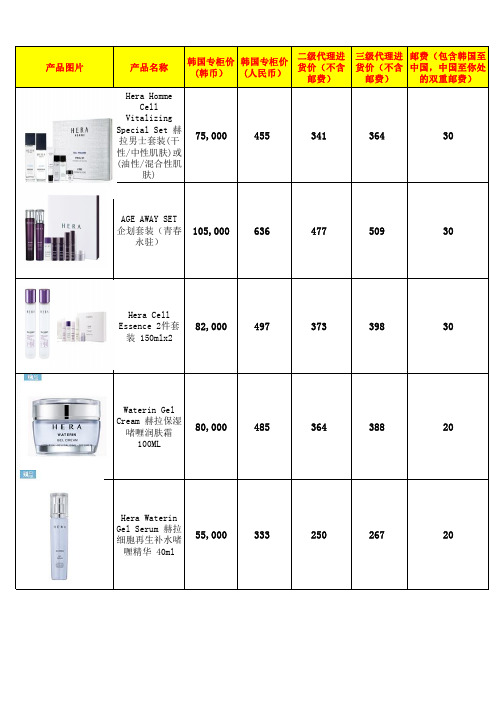
赫拉细胞再生保
湿水150ml
40,000
242
182
194
20
赫拉/HERA
赫拉细胞精华水 60,000
364
273
291
20
Cell Essence
150ML
赫拉/HERA
Cell-Bio-Cream 90,000
545
409
436
20
50ML 赫拉细胞
再生童颜霜
赫拉/HERA
HERA White
170
20
Emulsion 男士
细胞活力平衡爽
肤滋润乳液
赫拉/HERA
Waterin Roll-
on Eye Serum 45,000
273
205
218
20
水漾球状按摩眼
部精华 15ML
赫拉/HERA
White Program
Biogenic Cream 100,000
606
455
485
20
美白面霜 50ml
Foams 男士洁面
乳 150ml
赫拉/HERA
HERA HOMME
CELL
VITALIZING 50,000
303
227
242
20
MAGIC SKIN
CREAM 细胞活力
润肤霜 50ML
赫拉/HERA
White Program
Biggenic Powder Ampoule
150,000
909
682
产品图片
产品名称
韩国专柜价 韩国专柜价 (韩币) (人民币)
二级代理进 货价(不含
三级代理进 邮费(包含韩国至 货价(不含 中国,中国至你处
Inventory+Modeling+in+Supply+Chain+Management_+A+Review

Inventory Modeling in Supply Chain Management: AReviewCheng Tiexin Yue Jingbo Guo TaoCollege of Management, Tianjin Polytechnic University, Tianjin, China 300384tiexincheng@Abstract—In supply chain management, the inventory management of materials, semi-manufactured goods and products is often concerned and attracts a lot of scholars’ attentions. With the economy globalization, three new trends appeared in the supply chain management: materials procurement globalization, manufacture globalization and products distribution globalization. Consequently, three new areas in inventory modeling were paid more attentions to: 1. Multiple supplier and multi-product inventory models from the point of the upstream of the supply chain; 2. Multi-echelon inventory models including manufacturers, dealers and retailers from the point of the interior structure of the supply chain; 3. Stochastic multi-product demand inventory models from the point of the downstream of the supply chain. In this paper, the three areas mentioned above were discussed in detail and some new inventory models and researches were reviewed, and at the end of the paper, the research directions of the inventory management in supply chain management were given.Keywords-Supply chain, Inventory management, Multi-echelon inventory, forecastingI.I NTRODUCTIONIn supply chain management, inventory management about materials, semi-manufactured goods and products was widely focused on, and specialists and scholars all over the world have made a lot of researches on this area, especially for establishment of the inventory model. In 1915, when the first constant inventory model for the single product was set up, Ford. W. Harris established the model of EOQ (Economic Order Quantity), subsequently the researches on this area proceeded rapidly. With the economy globalization, three new trends appeared in supply chain management: materials procurement globalization, manufacture globalization, and products distribution globalization. Consequently, three new areas in inventory modeling were paid more attentions to: 1. Multiple supplier and multi-product inventory models from the point of the upstream of the supply chain; 2. Multi-echelon inventory models including manufacturers, dealers and retailers from the point of the interior structure of the supply chain; 3. Stochastic multi-product demand inventory models from the point of the downstream of the supply chain. In this paper, the new status and results of the research in this area will be reviewed in detail from the mentioned three trends.II.M ULTI-SUPPLIER AND MULTI-PRODUCT INVENTORYMODELSAbout the research on multi-supplier, Sculli & Wu[1] set up one model, in which two suppliers were introduced, and assumed that the lead time of the demand of products was Normal Distribution. According to this model, it was argued that the two suppliers had the same the replenishment quantity. Moinzadeh & Nahmias[2] established the inventory model with the continuing lead time for two suppliers, in which it was assumed (1) the two suppliers had the samecontinuous lead time (120ll<<) and different prices(21pp>); (2) the order costs: 21,CC; (3) shortages were allowed but the loss were aroused. The goal of the model was minimize the average inventory cost, which was determined by the order cost, storage costs and shortage loss, for long term, and according to that model the optimal replenishment policy ),,,(2121QQss was obtained. Based on the storage quantity t x at time t, the strategy is to order the quantity of goods (Q1) to supplier 1 when the t x was equal to the trigger level (s1) at time t, and to order the quantity of goods (Q2) to supplier 2 when the t x was equal to the emergency trigger level (s2) within the time l1, which was the lead time of Q1, before the Q1 occurred.Moinzadeh & Schmidit[3] studied the model set up by Moinzadeh & Nahmias[2], and modified it. They divided the optimal replenishment policy into two ways: the regular order (Q1) and the emergency order (Q2). In their revised model, when the demand occurs, (1) if 1+≥etSx (where: t x denotes the storage quantity of goods at time t;e S denotes the emergency trigger level), then the regular order (Q1) isapplied, (2) if etSx≤and the replenishment time of the regular order is less than the lead time of supplier 2, then theregular order (Q1) is applied, too, and (3) if etSx≤ and the replenishment time of the regular order is less than the lead time of supplier 2, then the emergency order is applied, that is to order the quantity of goods (Q2) to supplier 2.Chiang & Gutierrez[4] set up one model of two supply modes with periodic check for supplier, in their model, the cost of the emergence order was divided into two situations: C=0 and C>0, they applied dynamic programming to optimize the model, and the optimized policy was: when the inventorySponsored by Tianjin Municipal Science and Technology Commission, Project ID: 08JCZDJC24200.Cheng Tiexin: Ph.D of Management Science and Engineering, Associate Professor, Research areas: Project Management, Knowledge Management, Supply Chain Management Tel: 0086-22-83956951.was checked, if e t S x ≥, the regular order was applied; orelse if e t S x <, the emergency order was applied. In 1998, Chiang & Gutierrez extended the model above. In the new model, it assumed that the check cycle was continuous other than periodic and the cost of order was alterable not fixed. The models mentioned above belong to the models of two suppliers or two supply modes, however, Dayani Sedarage, Okitsugu Fujiwara & Huynh Trung Luong[5], and Ram Ganeshan[6] introduced the multi-supplier (N suppliers) in their inventory models, discussed the models of the multi-supplier (N suppliers) in detail and gave the optimized policy for inventory control.Considering that the uncertainties, such as the failure of the equipments, the strike of workers, the adverse climatic conditions and so on, would affect the suppliers to supply the goods on time, in 1996, Parlar & Perry[7] set up the model, in which they assumed that the goods were exchangeable and put one status variable, the value of which was ON or OFF (ON means to supply and OFF means not to supply), to every supplier. If the number of the suppliers was n , then there would be 2n combinations of suppliers, then they optimized the model to get one policy for ordering: (s i ,Q i ), where the reorder point s i was related with the order quantity Q i and the status variable of the suppliers.III.M ULTI -ECHELON INVENTORY MODELSThe economy globalization resulted in the globalization of manufacture and sale, therefore the multi-echelon inventory management was paid more and more attentions. According to the features of the multi-echelon inventory, we divided it into 3 types: (1) Serial inventory systems, (2) Assembly inventory systems and (3) Distribution inventory systems. About the multi-echelon inventory, Clark and Scarf[8] introduced the concept of echelon stock as opposed to installation stock. In echelon stock policies, ordering decisions at a given stage are based on the echelon inventory position, which is the sum of the inventory position at the considered stage and at all the downstream stages. They proved that there existed the optimal base stock ordering policy in the pure serial inventory systems, and developed one effective decomposing method to compute the optimal base stock policy. In addition, they also discussed the distribution inventory system and gave an approximate method for it. Federgruen & Zipkin[9] extended the model established by Clark & Scarf from the finite horizon to the infinite horizon with stationary parameters and developed an efficient computational method. Hochstaedter extended the model established by Clark & Scarf from the pure serial inventory system to the distribution inventory system, and Rosling[10] extended the model established by Clark & Scarf to the assembly inventory system and gave the method to get the optimal base stock policy of it.Generally, there are different ways to manage multi-echelon inventory systems. When the strategy of “one for one” is taken, installation stock policies can be proper, which means that the multi-echelon inventory control policy is the same as the installation stock policy. According to the current storage quantity of goods, the order policy of the multi-echeloninventory system can be obtained through calculating the total order quantities of the suppliers. However, if the times and quantities of the orders are very large, the strategy of “one for one” usually can not ensure the optimization for the inventory management. Axsäter & Rosling[11] proved that in serial and assembly inventory systems echelon stock policies achieved better performance than installation ones do, but in the distribution inventory system, these two policies had different advantages respectively. Axsäter & Rosling considered a two-echelon distribution inventory system with stochastic demand, proved that optimization of continuous review (R ,Q )-policies were usually very efficient in case of relatively low demand, and gave a method by which a high-demand system was approximated by a low-demand system. Tetsuo Iida[12] studied a dynamic multi-echelon inventory problem in the finite horizon, and gave the near-myopic policies which were sufficiently close to the optimal one and also could be applied to the distribution system.IV.T HE INVENTORY MODELS FOR STOCHASTIC MULTI -PRODUCT DEMANDThe classical EOQ model is based on the constant demand, and it is assumed that demand is continuous and even. If R stands for the rate of demand (demand quantity per time), which is constant, then the demand quantity in the time of t is Rt . But, in the real market, the product demand is dynamic and stochastic with the respect of the change of the price and time etc. At present, there are several kinds of the methods to forecast the products demand mainly as follow:A. The model of EconometricsThe demand is the function of the time (t ) in common econometrical forecasting models. In the classical EOQ model as mentioned above, the assumption is that demand function (Q =Rt ) is the linear function of time variable. Silver and Meal[13] studied the inventory model of the demand function of time (t ), and they proposed a heuristic algorithm which can be applied in most EOQ models. Donaldson[14] discussed the conditions in detail that the inventory horizon is finite and demand function is the linear function of time variable, and proposed the optimal reorder point. In addition, other scholars, such as Ritchie[15], Buchanan[16], Mitra et al.[17], Goyal[18], studied this kind of inventory models. The inventory model discussed above possessed the linear demand function which can change along with the time variable, however in the real market, the assumption of linear demand is so simple that it is far from the actual situation, hence some scholars turned to the non-linear demand function. Hariga and Benkherouf[19] established the inventory model in which demand function is the exponential function of time variable, considered the loss of shortages, and proposed the optimal policy of inventory replenishment on the condition that shortages were not allowed. Wee[20] also established the inventory model with the demand of the exponential function of time, it’s different from Hariga and Benkherouf, he proposed the optimal policy of inventory replenishment on condition that shortages were allowed. Considering that some demands of products (like computer chips and the aircraft components) grow rapidly for the new products and drop rapidly for the outdated products,S. Khanra and K.S. Chaudhuri[21] took the quadratic function of the time variable as the demand function, and established the corresponding inventory model.B.The model of Time SeriesThe model of time series is one common model, which can be applied to forecast most of products’ demand. The classical Gaussian Automatic Regressive Model (G.E.P. Box, G.M. Jenkins[22]), which is usually called the AR model, is applied widely in the commercial forecasting. Holt-Winters (HW) model (Holt, 1957; Winters, 1960) introduced exponentially weighted Moving Average models, which is usually called the MA model, to forecast the inventory demand, whereas Don M. Miller and Dan Williams[23] introduced the method of Ratio-to-Moving-Average Decomposition to do it, which can eliminate the seasonal influence to the demand. Lisa Bianchi, Jeffrey Jarrett and R. Choudary Hanumara[24] forecasted demand of the telecommunication market with Automatic Regressive Integrated Moving Average models (ARIMA), and contrasted the results with the Holt-Winters(HW) model. Moreover, S. L. Ho and M. Xie[25] analyzed the reliability of ARIMA model, Xiaolong Zhang[26] discussed how to eliminate the bullwhip effect in supply chain with different forecasting methods of time series, and proposed a simple rule to select different forecasting model.A combined forecast might improve upon the better of the two individual forecasts. Alternatively, combinations with other statistical forecasting methods might be advantageous. The concept of combining forecasts started with the seminal work of Bates and Granger[27]. Given two individual forecasts of a time series, they demonstrated that a suitable linear combination of the two forecasts may result in a better forecast than the two original ones, in the sense of a smaller error variance. Newbold and Granger[28], Makridakis et al.[29], have reported empirical results that showed that combinations of forecasts outperformed individual methods. Throughout the years, applications of combined forecasts have been found in many fields such as meteorology, economics, insurance and forecasting sales and price, see Clemen[30]. Chi Kin Chan, Brian G. Kingsman and H. Wong[31] described a case study of demand combining forecasting for inventory management, besides comparing performances between combination forecasts and individual forecasts. They also investigated the differences between regular changing weights and constant weights for a certain forecast horizon, finally gave the optimal stock policy.C.The Stochastic demand modelsThe classical newspaper boy model belongs to the inventory models of the stochastic demand. It is often assumed that the product demand is one kind of probability distributions, for example, the demand of discrete products is often supposed to obey the Possion distribution, and the demand of continuous products obeys the Normal distribution (Chiang and Benton[4]) etc. Ignall and Veinot proposed the inventory problem of stochastic multi-products during 1960's; subsequently, Goyal[18], Rosenblatt and Rothblum[32], Anily[33] did further researches for the inventory problem of stochastic multi-product demands and established some mathematical models, most of their researches are based on the classical EOQ model. Canadian scholar Dirk Beyer, Suresh P. Sethi and R. Sridhar[34] proposed the stochastic multi-products inventory model, which was set limit to the capacity of the inventory on the foundation of aforementioned researches, this model was the improvement of hereinbefore models.In addition, some scholars applied the Bayes method to revise the forecasting outcome of the stochastic product demand, e.g. K. Surekha and Moheb Ghali[35], K. Rajashree Kamath and T. P. M. Pakkala[36] analyzed the problem of inventory demand of Stationary and Non-Stationary, and obtained more reasonable optimized inventory policy with Bayes forecasting method.V.T HE NEW RESEARCH DIRECTIONS FOR INVENTORYMODELINGA.Integrated inventory modelingAt present, supply chain management has the trend to integration; more and more manufacturers in the supply chain form the strategic alliance. Inventory management is also in the direction of integration. Consequently, the single manufacturer or supplier has to establish integrated inventory model in view of the supply chain from upstream to downstream when they make decision of the inventory management, and multi-echelon inventory modeling needs to be applied.B.Internet and E-business based virtual inventory modelingWith the development and application of the Internet and E-business in supply chain, the purchase and order costs between buyers and sellers are decreasing, and the risks of suppliers are being reduced. This results in that multiple suppliers’ pattern is superior to single supplier pattern. The development of IT causes information-sharing between the buyers and the sellers. Buyer’s demand can be forecasted based on the information of the venders, however, suppliers should deal with a great deal of data. Therefore, Data Mining and Knowledge Discovery in Database have the wide application prospects in inventory management; in the meanwhile, more attentions will be paid to virtual inventory modeling.C.Inventory modeling under asymmetric informationIn the real supply chain, every partner (manufacturer or supplier) makes his decision independently, hence there exits asymmetric information. Even if the coordination has been set up in supply chain, the partner usually keeps his commercial information, such as costs, profits and so on, in secret, which leads to that it is difficult to get this information for other partners. Therefore, inventory modeling under asymmetric information is more valuable and practicable. There are some researches on this field, in which the game theory was often applied to decision-making under asymmetric information; however it needs to be studied more intensively and extensively.VI.C ONCLUSIONIn this paper, three types of inventory models were discussed from the aspects of supply chain management:(1)Multi-supplier and multi-product inventory model;(2)Multi-echelon inventory model; (3)Stochastic multi-product demand inventory model. The research history and development of the inventory models were reviewed and the latest research results were discussed. Finally, the future research directions of the inventory management in supply chain management were given. The inventory management was under way of integration, the IT and Internet will be considered and paid more and more attentions to inventory modeling, and inventory modeling under asymmetric information will become more valuable and practicable.R EFERENCES[1]Sculli, D., Wu, S.Y.,. Stock control with two suppliers and normal leadtimes. Journal of the Operational Research Society, 32(11), 1981, 1003-1009.[2]Moinzadeh, K., Nahmias, S., A continuous review model for aninventory system with two supply modes. Management Science,1988(34): 761–773.[3]Moinzadeh, K., Schmidt, C.P., An (S-1, S) inventory system withemergency orders. Operations Research, 1991(39): 308-321.[4]Chiang, C., Beton, W.C., Sole souring versus dual souring understochastic demands and lead times, Naval Research Logistics 41,1994,609-624.[5]Dayani Sedarage, Okitsugu Fujiwara, Huynh Trung Luong,Determining optimal order splitting and reorder level for N-supplierinventory systems, European Journal of Operational Research 116(1999) 389-404.[6]Ram Ganeshan, Managing supply chain inventories:A multiple retailer,one warehouse, multiple supplier model, Int. J. Production Economics,59 (1999) 341-354.[7]M. Parlar and D. Perry, Inventory models of future supply uncertaintywith single and multiple sources. Naval Research Logistics,1996(43):191-210.[8] A.J. Clark, H.E. Scarf, Optimal policies for a multi-echelon inventoryproblem, Management Science, 6(1960) 475-490.[9]Federgruen, P. Zipkin, Computional issues in an infinite-horizon multi-echelon inventory model, Operations Research, 32 (1984)818-836. [10]K. Rosling, Optimal inventory policies for assembly systems underrandom demands, Operations Research, 37(1989)565-579.[11]Axsäter and Rosling, Installation vs. echelon stock policies for multi-level inventory control, Management Science, 39 (1993) 1274-1280. [12]Tetsuo Iida, The infinite horizon non-stationary stochastic multi-echelon inventory problem and near-myopic polices, European Journalof Operational Research, 134(2001)525-539.[13]Silver EA, Meal HC. A simple modification of the EOQ for the case ofa varying demand rate. Production and Inventory Management,1969;10(4):52-65.[14]Donaldson WA. Inventory replenishment policy for a linear trend indemand—an analytical solution. Operational Research Quarterly, 1977;28:663-70.[15]Ritchie E. Practical inventory replenishment policies for a linear trendin demand followed by a period of steady demand. Journal ofOperational Research Society, 1980;31:605-13.[16]Buchanan JT. Alternative solution methods for the inventoryreplenishment problem under increasing demand. Journal ofOperational Research Society, 1980; 31:615-20.[17]Mitra A, Fox JF, Jessejr RR. A note on determining order quantitieswith a linear trend in demand. Journal of Operational Research Society,1984;35:141-4. [18]Goyal SK. On improving replenishment policies for linear trend indemand. Engineering Costs and Production Economics, 1986; 10:73-6.[19]Hariga MA, Benkherouf L. Optimal and heuristic inventoryreplenishment models for deteriorating items with exponential time-varying demand. European Journal of Operational Research,1994;79:123-37.[20]Wee HM. A deterministic lot-size inventory model for deterioratingitems with shortages and a declining puter and Operations Research, 1995; 22(3):345-56.[21]S. Khanra, K.S. Chaudhuri, A note on an order-level inventory modelfor a deteriorating item with time-dependent quadratic demand,Computers & Operations Research, 30 (2003) 1901-1916.[22]G.E.P. Box, G.M. Jenkins, Time Series Analysis: Forecasting andControl, Seconded Edition., Holden-Day, San Francisco, 1976. [23]Don M. Miller , Dan Williams, Shrinkage estimators of time seriesseasonal factors and their effect on forecasting accuracy, International Journal of Forecasting, 2002.[24]Lisa Bianchi, Jeffrey Jarrett, R. Choudary Hanumara, Improvingforecasting for telemarketing centers by ARIMA modeling withintervention, International Journal of Forecasting, 14 (1998) 497-504.[25]S.L. Ho and M. Xie, The use of ARIMA models for relliablityforcasting and analysis, Computers and Electrical Engineering, 1998,Vol. 35, 213-216.[26]Xiaolong Zhang, The impact of forecasting methods on the bullwhipeffect, Int. J. Production Economics, 2004(88):15-27.[27]Bates, J.M., Granger, C.W.J., The combination of forecasts.Operational Research Quarterly, 20(1969.) 451-468.[28]Newbold, P., Granger, C.W.J., Experience with forecasting univariatetime series and the combination of forecasts (with discussion). Journal of the Royal Statistical Society Series A, 137(1974), 131-149. [29]Makridakis, S., Winkler, R.L., Averages of forecasts: Some empiricalresults, Management Science, 29(1983), 987-996.[30]Clemen, R.T., Combining forecasts: A review and annotatedbibliography. International Journal of Forecasting, 5(1989), 559±583.[31]Chi Kin Chan, Brian G. Kingsman, H. Wong, The value of combiningforecasts in inventory management-a case study in banking, European Journal of Operational Research, 117 (1999) 199-210.[32]Rosenblatt, M. J. and Uriel G. Rothblum, The Single Resource Multi-item Inventory Systems, Operational Research, 1990, 38, 686-693. [33]Anily S, Multi-Item Replenishment and Storage Problems(MIRSP):Heuristics and Bounds, Operational Research, 1991, 39, 233-239. [34]Dirk Beyer, Suresh P. Sethi, R. Sridhar, Stochastic Multi-ProductInventory Models with Limited Storage, work paper, University ofToronto, Ontario, Canada,1997.[35]K. Surekha, Moheb Ghali, The speed of adjustment and productionsmoothing: Bayes estimation, Int. J. Production Economics, 71(2001)55-65.[36]K. Rajashree Kamath,T. P. M. Pakkala, A Bayesian approach todynamic inventory model under an unknown demand distribution,Computers & Operations Research, 29(2002): 403-422.Inventory Modeling in Supply Chain Management: A Review作者:Cheng Tiexin, Yue Jingbo, Guo Tao作者单位:College of Management, Tianjin Polytechnic University, Tianjin, China 300384本文链接:/Conference_WFHYXW331993.aspx。
诺贝尔2012年价格
309*459 150*150 350*350 211*211 150*150 100*309 50*309 50*50 50*309 50*20 150*309 309*609 120*309 20*120 300*300 600*600 600*600 200*300 200*200 600*600 200*200 200*200 200*200 600*600 100*100 100*100 100*100 100*100 600*600 600*400 200*200 145*600 145*145 120*400 120*120 70*300 70*28
C CN66206
HL7065206 HL12065206 CN66207 CN65207 CN22207 66207L1 66207L2 CN66207 KL7065207 HL2865207 HL7065207 CN66208
CN66208 CN66209 CN66209 66208S
70*30 20*120 600*600 600*400 200*200 145*600 145*145 70*300 70*28 70*30 600*600 600*600 600*600 150*600 150*150 600*600 400*600 200*200 800× 800 450*450 150*450 150*150 450*450 150*450 150*150 450*450 50*50 50*50 50*50 450*450 50*50 50*50 50*50 300*300 150*300 150*150 300*300 300*300
Q46955 Q46956
印象瓷片系 列
Q46960 Q46961
TL15046960
Firms_as_surrogate_intermediaries

Firms as Surrogate Intermediaries:Evidence from Emerging Economies∗Hyun Song Shin†Laura Yi Zhao‡December2013AbstractAfirm canfinance investment either by borrowing or by drawing on cash balances, so thatfinancial asset and liability changes tend to have opposite signs.In contrast,financial intermediaries borrow in order to lend,so thatfinancial asset and liabilitychanges have the same rge non-financialfirms in China and India behave likeintermediaries rather than textbook non-financialfirms.We explore the role of non-financialfirms in the shadow banking system.The evidence from China and India isin contrast to US non-financialfirms,which conform to the textbook predictions.∗Preliminary.This study forms part of the background research for the Asian Development Bank technical assistance program on“Financial Regulatory Reform in Asia”.†Corresponding author:Bendheim Center for Finance,Princeton University,26Prospect Avenue,Prince-ton,NJ08540,USA;hsshin@‡Asian Development Bank;yzhao.consultant@1IntroductionThe market stresses faced by many emerging economies in the face of tighter global monetary conditions in2013have focused renewed attention on the transmission offinancial conditions across borders.One conceptual challenge is to reconcile the small net external debt positions of many emerging economies with the apparently disproportionate impact of tighter global monetary conditions on their currencies andfinancial markets.Indeed,some commentators have wondered aloud why emerging economies with low net external debt positions are experiencing such severe stresses.1The purpose of our paper is to offer one missing piece in the puzzle,highlighting the role of non-financial corporations as surrogatefinancial intermediaries that operate across borders.When corporate activity straddles the border,measuring exposures at the border itself may not capture the strains on corporate balance sheets.For instance,if the London subsidiary of the company has taken on US dollar debt but the company is holding domestic currencyfinancial assets at its headquarters,then the company as a whole faces a currency mismatch and will be affected by currency movements,even if no cross-border exposures are registered in the official net external debt statistics.Nevertheless,thefirm’s fortunes (and hence its actions)will be sensitive to currency movements.In the case offirms that straddle borders,it may be more illuminating to look at the consolidated balance sheet that motivates corporate treasurers,rather than the balance of payments statistics that are organized according to residence.One aspect offirms’access to international capital markets is the offshore issuance of debt securities sold to international investors.If the debt securities issued offshore are in foreign currency,offshore issuance would mirror currency mismatches on the consolidated balance sheet.Hence,offshore issuance goes beyond just a measurement issue on the size of the company’s debt and instead addresses the fundamental issue of howfirms will fare when 1For instance,Krugman(2013)“Asian Vulnerability,Then and Now”/2013/08/29/asian-vulnerability-then-and-now/1B i l l i o n U S d o l l a r sB i l l i o n U S d o l l a r s Figure 1:China (left)and India (right):International debt securities outstanding for non-financial corporates by nationality and by residence (Source:BIS Debt Securities Statistics,Table 11D and 12D)global financial conditions and exchange rates change.Figure 1shows BIS statistics on the amounts outstanding of international debt securities issued by non-financial corporate borrowers in China (left)and India (right)by residence of the borrower (blue)and the nationality of the borrower (red).The difference between the red and blue series reflects the offshore issuance of corporate debt securities.We see from Figure 1that offshore issuance activity was small until the 2008crisis,but subsequently grew strongly.The period after 2010has seen a particularly steep increase so that by 2013,the offshore amounts outstanding are equal in size to the onshore issuance outstanding.McCauley,Upper and Villar (2013)describe the recent trend of offshore issuance of corporate debt securities.2Our paper examines the role of the firm as a surrogate financial intermediary that trans-mits financial conditions across borders.The hallmark of banks and other financial inter-mediaries is that they borrow in order to lend.As such,when their financial assets increase through new lending or purchases of securities,their financial liabilities,such as deposits,also increase.In this way,a distinctive feature of financial intermediaries is that the change in their financial assets has the same sign as the change in their financial liabilities.In contrast,textbook non-financial firms behave in a very different way.When a non-Agust´ın Villar “Emerging market debt securities issuance in offshore centres”BIS Quarterly Review,September 2013,Box 2,pp 23-24./publ/qtrpdf/r qt1309b.pdf 2financialfirm undertakes an investment,it canfinance it either by drawing on its existing financial resources or by external borrowing,or a combination of both.A prediction of the “pecking order”theory of corporatefinance(Myers(1984))is that thefirm will draw on internal fundsfirst as the cheapest form offinancing,and only tap outside funding when internal funds are inadequate.A prediction from such behavior would be that changes in financial assets and changes infinancial liabilities will have opposite signs,capturing those firms that raise outside funding while drawing down internal funds.We show that non-financialfirms in emerging economies behave likefinancial intermedi-aries in that co-movements infinancial assets andfinancial liabilities have a positive sign. This is true both in the cross-section,as well as in the time series.In other words,firms that borrow more also hold more cash,andfirms that increase their borrowing also increase their cash holding.To the extent thatfirms’cash holdings are claims on the domestic bank-ing sector,thefirms would be performing afinancial intermediation role by making funding available indirectly to other domestic borrowers.Our paper has a close parallel with Hattori,Shin and Takahashi(2009),who describe the role of non-financial corporates as surrogate intermediaries in Japan in the1980s.Hattori et al.(2009)show how thefinancial liberalization of the1980s enabled large manufacturing firms in Japan to gain access to funding by issuing securities,especially from international investors who sought yen exposure.As new funding sources opened up,firms recycled yen funding through the banking system in the form of bank time deposits.Through this channel, thefinancial assets of non-financialfirms increased in step with theirfinancial liabilities in the1980s.Banks in Japan suffered a reversal of roles in which corporate borrowers became corporate depositors,and banks were pushed to seek borrowers in riskier sectors such as in commercial real estate.The parallel between Japan in the1980s and the emerging economies in2013lies in the role of non-financial corporates as surrogate intermediaries.The evidence in our paper comes from a large panel of non-financialfirms emerging economies in the Compustat Global database in which we examine both the cross-section3patterns in corporate balance sheets,as well as the growth of individualfirms’financial assets and liabilities withfirmfixed effects.The evidence from the major emerging economies is especially noteworthy given its contrast to US non-financialfifirms are seen to conform to the textbook prescription for corporatefinancing choices in whichfinancial assets and liabilities move in the opposite directions,consistent with the pecking order theory of financing(Opler et al.(1999)).Our paper has a point of contact with the many studies that have explored the trends and implications of corporate cash holdings.Traditional studies focus onfirm value,merges and acquisitions,and dividend issuance.Harford(1999)shows that cash-richfirms are more likely to attempt acquisition and their mergers tend to be followed by a decline in operating performance.Lie(2000)finds that a large increase of dividends mitigates the agency problem associated with excess cash-holdings.Denis and Sibilkov(2010)show that as due to costly externalfinancing,greater cash holdings increase the value of constrainedfirms.Our paper contributes to this literature by exploring the implications of the non-financialfirms’cash holdings for the liquidity in the banking system.Given the importance of corporate liquidity,many works explore its determination.Opler et al.(1999)and Ferreira and Vilela(2004)find supportive evidence for a static trade-offtheory using data from the United States and European countries respectively.Bates et al. (2009)argues that precautionary motives explain the rise of US industrialfirms’cash-to-asset ratio.The role of corporate governance is also explored.As an example,Dittmar et al.(2003)finds that the agency problem is an important determinant of corporate cash holdings,and thatfirms in countries with poor shareholder rights hold twice as much cash asfirms in countries with good shareholder protection.Other factors are also found to affect corporate liquidity:tax cost for multinational companies to repatriate foreign income(Foley et al.(2007)),the predation risk(Haushalter et al.(2007)),the diversification of investment opportunities(Duchin(2010)),and the incentive to hedge cashflow shocks during bad times (Lins et al.(2010)).Adding to this line of literature,our paper explores a new perspective4to understand non-financialfirms’cash holdings through their role as surrogatefinancial intermediary.Our paper is also related to the studies on thefinancing decisions offirms,in particular the use of debtfinancing.This line of literature focuses on two competing theories:the trade-offtheory and the pecking order theory.The empirical evidence is mixed.Shyam-Sunder and Myers(1999)argues that the basic pecking order model has more explanatory power than the static trade-offtheory in explaining thefinancing patterns of public and maturefirms in the United States.On the other hand,Frank and Goyal(2003)and Fama and French(2005)find pervasive evidence contradicting the pecking order ter on, Leary and Roberts(2010)show that the pecking order theory performs better in explaining firms’financing decisions only when factors typically attributed to other theories are simul-taneously accounted for.These two theories focused mainly on the traditional explanations for corporate use of debt,for example taxes,bankruptcy cost,transaction costs,adverse selection and agency conflicts.Our paper,by investigating the surrogatefinancial interme-diary roles of the non-financialfirms,suggests that the non-financialfirms in China borrows in order to invest,especially in the form of deposit and other short-term investments.Before documenting the key facts,we delve deeper into the institutions that underpin the empirical results.In particular,we explore how the availability offinancing from inter-national capital markets induces large non-financialfirms to engage infinancial transactions in the shadow banking system that have the tell-tale attributes offinancial intermediation. The institutional backdrop of the shadow banking system in China is a tightly regulated formal banking sector,which sits alongside a highly open and trade-dependent economy. Even if capital account transactions through banks can be tightly regulated,the current account transactions of thousands offirms generated in the course of international trade will be much harder to monitor and regulate.By its nature,shedding light on the shadow banking system andfirms’roles in the system presents formidable challenges in measurement and for data availability.However,5Figure2:Non-financialfirms as intermediary.In this diagram,firms with access to international capital markets act as an intermediary for outside funding when the banking sector has restricted access to international capital markets.the advantage of our approach is that,however thefirms managed to change theirfinancial claims and liabilities,the consequences of their actions will be captured in the snapshot of the consolidated balance sheet at the reporting period.As such,for the purpose of gauging the scale of intermediation performed by non-financialfirms,we can simply read offthe financial assets and liabilities,without having to capture in detail all the specific practices that thefirms engage in reaching theirfinal position.When the availability of externalfinancing from international capital markets varies with global liquidity conditions,a prediction of our approach is that the surrogatefinancial intermediation activity of non-financialfirms in emerging economies will reflect(at least in part)the ebb andflow of global liquidity conditions themselves.Consistent with this hypothesis,wefind that the extent of intermediation activity of non-financialfirms co-moves strongly with indicators of credit availability at the global level.We contrast the evidence from emerging economyfirms andfirms from the United States.While USfirms conform closely to the textbook model,firms from emerging economies exhibit the distinctive positive co-movement offinancial assets and liabilities.We conclude with some broader lessons for the operation of thefinancial system in a tightly regulated economy.6Chinese corporate Hong Kong bankFigure3:Offshore borrowing by a non-financial corporate in foreign currency2BackgroundAn economy with an openfinancial sector and convertible capital account will be sensitive to globalfinancial conditions,but the sensitivity to externalfinancial conditions also applies to economies that are tightly regulated and whose capital accounts are closed.Just as water willfind cracks to trickle through a rock,so will international capitalfind ways into an open economy when it has a large volume of transactions associated with trade.This is so even when thefinancial sector is tightly regulated and external borrowing is restricted by regulations that govern capital inflows.The role of non-financialfirms is crucial in this respect as the channel through which capital inflows take place.Figure2depicts an economy with a banking sector that has restricted access to wholesale funding in international capital markets,but where a subset offirms have access both to the domesticfinancial system as well as international capital markets through tradefinancing or the operation of overseas offices.Although non-financialfirms are subject to regulations in their use of international capital markets,the sheer number of suchfirms as well as the complexity of their transactions make them much harder to regulate than the banks.As well as the corporate bond market,global banks provide another channel to the international capital markets.Figure3is a schematic illustration of the activities of a non-financialfirm from China7-400-300-200-100100200300400Jan-2003Oct-2003Jul-2004Apr-2005Jan-2006Oct-2006Jul-2007Apr-2008Jan-2009Oct-2009Jul-2010Apr-2011Jan-2012B i l l i o n H K d o l l a r s Claims on non-bank customers in China (F.C.)Liabilities to non-bank customers in China (F.C.)Figure 4:Hong Kong banks’claims and liabilities to non-bank customers in China in currencies other than Hong Kong dollars (Source:Hong Kong Monetary Authority)with operations in Hong Kong,who borrows in US dollars from an international bank in Hong Kong and posts Renminbi deposits as collateral.The transaction would be akin to a currency swap,except that the settlement price is not chosen at the outset.The transactions instead resemble the operation of the old London Eurodollar market in the 1960s and 70s.For the Chinese corporate,the purpose of having US dollar liabilities and holding the proceeds in Renminbi may be to hedge their export receivables,or simply to speculate on Renminbi appreciation.Figure 4provides some aggregate evidence for the transactions depicted in Figure 3.Figure 4plots the claims and liabilities of Hong Kong banks in foreign currency to customers in China.Foreign currency,in this case,would be US dollars mainly for the assets and Renminbi mainly for the liabilities.Both have risen dramatically in recent years,reflecting the rapidly increasing US dollar funding of non-financial corporates from China.As well as channeling capital flows into China,non-financial firms play a more direct role as a financial intermediary through the institution of “entrusted loans”.Entrusted 8Figure5:Non-financialfirms as intermediary through“entrusted loans”.This diagram depicts the operation of“entrusted loans”where non-financialfirms lend to other non-financialfirms with limited access to bank lending.The bank acts as delegated manager of the loan contract.loans are loans granted by onefirm to anotherfirm directly.However,a commercial bank administers the loan as a delegated manager.Figure5illustrates the operation of an entrusted loan,where a largefirm with access to bank loans recycles the loan by granting an entrusted loan to anotherfirm-typically a smallerfirm with restricted access to bank lending,or a property-relatedfirm.The commercial bank administers the entrusted loan, and the entrusted loan stays offthe bank’s balance sheet,and hence does not count against lending limits set for the commercial bank by the bank regulators.From Figure5,we see that the lendingfirm in the entrusted loan relationship behaves like afinancial intermediary, simultaneously borrowing and lending.Increased incidence of such intermediation activity will be captured in a snapshot of the lendingfirm’s balance sheet as the simultaneous increase in bothfinancial assets andfinancial liabilities.Quantitatively,the intermediation conducted through entrusted loans is large relative to the lending through the formal banking sector.Figure6plots the quarterlyflow of entrusted loans and domestic currency bank loans in China,as published by the People’s Bank of China statistics on all systemsfinancing(also called total socialfinancing).We see that theflow of entrusted loans have increased in recent quarters,reaching25%to30%of90.00.51.01.52.02.53.0T r i l l i o n R M B0%5%10%15%20%25%30%Figure 6:Quarterly flow of entrusted loans and Renminbi bank loans (Source:People’s Bank of China,/publish/diaochatongjisi/4032/index.html)formal bank lending in China.3DataWe now turn to our empirical analysis,starting with a description of the data used in our study.The activities illustrated in Figures 5and 2suggest that the transactions underlying the surrogate intermediation done by non-financial firms can be complex and not easy to disentangle.Nor are these transactions easily measured or monitored.Our strategy,therefore,is to focus on the snapshot of the balance sheet at the end of the year,and investigate the co-movement in financial assets and financial liabilities of the firms,both in the cross-section and over time for each firm individually.Our firm level data comes from Compustat Global.The advantage of this data is two-fold.First,the database includes listed firms in China,which would include the largenon-financial firms that would be candidates for the intermediation activity described so far.Since we are interested in the firms engaged in the surrogate intermediation rather than the small and medium sized enterprises that are the ultimate borrowers,confining attention to10the largefirms will not miss the bulk of the surrogate intermediation.Second,Compustat Global imposes accounting classifications that are designed to ensure that cross-country comparisons are possible.Cross-country comparability is important for our purpose,as one of the checks to our main investigation is to compare the empirical results for China with that for the United States.For such an exercise,cross-country comparability is crucial,and Compustat Global ensures broad comparability.3.1Firm level data for ChinaOur sample offirms from China in Compustat Global covers thosefirms with Global Industry Classification Standard(GICS)sector codes not equal to40.The sample period is from1990 to2012,with data cutoffdate as November30,2013.For our benchmark regressions,we exclude thefirms which are outliers in terms of the ratio of cash and short-term investments to sales(above the99.5or below the0.5percentiles).After the sample selection,there are 1532firms in our sample.As our focus is on the surrogate intermediation activity offirms,our focus is on the cash and short-term investment position of thefirms,as well as otherfinancial assets.In what follows,“cash”is taken to mean cash and short-term investments.Financial liabilities are defined as the sum of the short—term debt and the long-term debt,which includes bank loans.Firm leverage is defined asfinancial liabilities divided by total assets.The summary statistics are presented in Table1.We note the following features.First,cash-holdings of Chinesefirms grew rapidly over the sample period.The average cash-holding increased more thanfive-fold from RMB248.6 million in1990to RMB1,488.3million in2012.Second,the growth of cash holdings was skewed to largefirms in the later periods,as suggested by the faster growth of the mean cash holding relative to the25and75percentiles. Therefore,the rapid growth of the averagefinancial liabilities seems mainly to have been driven by largefirms.11Table1:Description of variables for the1990-2012Compustat sample for publicly traded Chinese non-financial companies.Cash includes short-term investments;financial liabilities are defined as the sum of the short—term debt and the long-term debt;firm leverage is defined asfinancial liabilities devided by totalper-centileper-centilefirms A.1990-2012cash879.871.4198.4501.1179931532financial liabilities1,911.1119.0318.1893.0179931532 sales5,374.2351.1832.92,252.6179931532firm leverage27.1%15.1%25.3%36.7%179931532 cash/sales31.5%10.4%19.9%37.9%179931532financial liabilities/sales59.3%19.0%39.2%72.4%179931532B.1990-2001(Period1)cash248.623.979.1205.84919775financial liabilities607.774.3170.0390.44919775 sales1,226.7192.2388.4838.34919775firm leverage26.7%16.3%25.6%35.6%4919775 cash/sales31.1%7.3%17.1%38.4%4919775financial liabilities/sales63.9%24.0%45.6%78.3%4919775C.2002-2007(Period2)cash662.686.5206.1455.258731260financial liabilities1,533.5164.0382.8915.358731260 sales4,509.0395.5878.12,214.658731260firm leverage28.6%17.1%27.0%38.0%58731260 cash/sales30.0%10.8%19.9%36.5%58731260financial liabilities/sales64.6%21.0%43.2%79.7%58731260D.2008-2012(Period3)cash1,488.3135.6354.0838.372011499financial liabilities3,109.5149.8447.21,450.072011499 sales8,912.8587.81,393.43,799.172011499firm leverage26.1%12.8%23.7%36.0%72011499 cash/sales33.0%12.0%21.2%38.7%72011499financial liabilities/sales51.9%15.2%32.3%62.0%7201149912Figure7:China:Ratio of aggregate cash to aggregate sales offirms in sample(positive bars)and ratio of aggregatefinancial liabilities to aggregate sales(negative bars)Third,cash holdings grew faster than sales,which in turn grew more rapidly thanfinancial liabilities.As a result,the ratio of cash to sales ratio has increased during the sample period, while the ratio offinancial liabilities to sales has fallen in the sample period.Figure7shows the cash to sales ratio andfinancial liabilities to sales ratio of the sample Chinesefirms.The chart indicates that the cash to sales ratio co-moved with thefinancial liability to sales ratio Figure8is the scatter plot of cash holdings versus sales,plotted in log scale.The slope of the scatter is close to1,suggesting that there is a roughly proportional relationship between cash holdings and sales,so that sales are a good normalizing variable forfirm size.A roughly proportion relationship between cash and sales would be consistent with a“buffer stock”view of cash holdings,wherefirms hold cash to serve as a buffer against shocks to cashflows.13Figure8:Scatter plot of cash vs sales in log scale for samplefirms in2000and2011.3.2Bond IssuanceAs well asfirm-level data,we will also employ aggregate corporate bond issuance series for non-financialfirms from China as an aggregate explanatory variable in the panel regressions. Aggregate corporate bond issuance serves as an indicator of the availability of credit through debt markets.When the corporate bond is issued in foreign currency,the issuance series also serves as an indicator of global capital market conditions and the availability of credit tofirms in China from international investors.Figure11shows the total outstanding amounts of bonds for different sectors in China. The chart uses total depository data from China Central Depository and Clearing Co.Cor-porate bonds grew from literally nothing to RMB5trillion between1997and2012.Even when the amounts are normalized relative to China’s GDP,we see from Figure10that the corporate bonds outstanding has increased very rapidly from only1%in2005to10%of China’s GDP by2012.Figure11shows the breakdown of total corporate bonds by instrument.The corporate bonds category encompasses commercial paper(CP)and medium-term notes(MTN),both of which are shorter maturity instruments.Medium-term notes(MTNs)have grown most14Figure9:Total bond depository amount of China.Source:China Central Depository and Clearing Co..Figure10:Total bond depository amount to GDP ratio in China.Source:China Central Depository and Clearing Co..15Figure11:Breakdown of total corporate bond depository amount.Source:China Central Depository and Clearing Co..significantly since their inception in2008,indicating the increasing need for medium-term financing for Chinesefirms By2012,MTNs accounted for over half of the total corporate bonds.Foreign currency bond issuance by Chinesefirms has also increased rapidly in recent years.The outstanding balance increased from USD4.7billion in2001to USD81.7billion in2012.Figure12plots the foreign currency bond outstanding relative to China’s GDP by sector.We see that private issuance byfirms was lower than the issuance by the government sector,but private issuance overtook government sector issuance in2008and has pulled away further since.As of2012,foreign currency corporate bonds outstanding is around1%of China GDP,while government bonds accounted for only0.25%.4Panel Regressions for ChinaWe proceed to examine panel regressions that ascertain howfinancial asset holdings vary with thefirm’sfinancial liabilities.16Figure12:Foreign currency bond outstanding to GDP ratio by government,financial institutions and other corporates.Source:Asian Development Bank.4.1Panel regressions in log ratiosOurfirst set of panel regressions are for log of cash(including short-term investments)to sales ratio regressed on log offinancial liabilities to sales ratio.Our interest is in the sign of the coefficient on log offinancial liabilities to sales ratio.We include log sales andfirm leverage,defined asfinancial liabilities to total assets,as control variables.We also include the full set of yearfixed effects andfirmfixed effects.Table2presents the regression results. We present results below on the case where we have dropped observations forfirms that have zerofinancial liability at any date in the sample.Qualitatively,the results are unchanged when we includefirms with zero debt,although the coefficient is smaller.Column(1)is for the full sample.We see that the sign on ln(fin liab)is positive and significant at the1%level.The coefficient of0.209implies that a1%increase infinancial liabilities to sales ratio in the cross-section translates into a0.21%increase in cash and short-term investment holdings to sales ratio.In columns(2)to(5),we examine subgroups offirms arranged into four size quartiles based on the average sales of thefirms over the period.As largefirms may have better17。
NEMA 4防水封闭式柜体购买指南说明书

Enclosures Right Now, Right Price.NEMA 4 Enclosures Buyer’s GuideThe first step in selecting a NEMA 4 enclosure is to make sure that you really need it. The definitions below will help you select the just-right NEMA rating for your application, like Goldilocks: neither too much nor too little.NEMA 1: For indoor use. Protects users against contact with hazardous components and protects the components from the ingress of solid objects, such as fingers and falling dirt.NEMA 2: For indoor use. Same as NEMA 1 but adds protection against the ingress of dipping and light splashing water.NEMA 3: For indoor or outdoor use. Same as NEMA 2 but adds stronger protection against the ingress of water and dust. It protects against windblown dust, rain, sleet, and snow and will be undamaged by ice forming on the enclosure.NEMA 3R: Same as NEMA 3 but without the protection against windblown dust.The standard doesn’t say this, but typically the difference is that there is no gasketingon NEMA 3R enclosures.NEMA 3S: Same as NEMA 3 but adds the provision that external mechanism remain operable when ice laden.NEMA 3X, NEMA 3RX, NEMA 3SX: the X signifies the addition of corrosion protection.NEMA 4: Same as NEMA 3 but adds protection against hose directed water.NEMA 4X: Same as NEMA 4 but adds protection against corrosion.NEMA 6: For indoor or outdoor use. Protects against the ingress of objects, fingers, and falling dirt, hose directed water and is undamaged by ice formation. What’s more,it protects against occasional temporary submersion to a limited depth.NEMA 6P: Same as NEMA 6 but adds protection of prolonged submersion to a limited depth and adds corrosion protection.NEMA 12: Protects against the ingress of objects, fingers, falling dirt, settling dust and drips. It is similar to NEMA 3 but it is for indoor use, so instead of protecting against windblown dust it protects against settling airborne dust, lint, fibers, and flyings. It won’t protect against rain, sleet, and snow, but it does protect against seeping oil and coolant as well as dripping and light splashing water. Despite the large number it is a basic level of protection. It may be helpful to think of it as NEMA 1.2 rather than NEMA 12.NEMA 13: Same as NEMA 12 but adds protection against oil and coolant splashing and spraying.By the way, the above definitions are for non-hazardous locations. NEMA 7, 8, 9 and 10 are the ones to look at for hazardous environments.Tips on Selecting a NEMA 4 EnclosureDo you need to protect the entire enclosure, or only a sensitive component? For example, if only one component needs NEMA protection, then protect that component with a small die-cast type NEMA box instead of buying a large NEMA 4 enclosure.What level of protection is required? The most common mistake is to specify a NEMA 12 enclosure, when in fact NEMA 4 enclosures offers more environmental protection. On the other hand, don’t over specify, because each increasing level of protection can exponentially increase the cost of an enclosure. Consider where the enclosure will be located. Often a NEMA 12 enclosure will work if there is no spray down requirement. There is no point to specifying UV stabilization if the plastic enclosure is being used indoors.What material do you need? Steel is often the choice for a NEMA enclosure, especially for large enclosures where its strength is helpful. However, plastic is less costly and provides adequate protection in many applications. Polycarbonate plastic, ABS plastic, fiberglass, and die cast-aluminum enclosures are lower cost materials than steel and should not be overlooked. Plus they are inherently corrosion resistant.ABS plastic is tough stuff; NFL helmets are made of ABS. Polycarbonate plastic has the option of being transparent—ideal for viewing readouts without breaking the seal. Relatively new is a polycarbonate infused with 10 percent fiberglass. The fiberglass helps assure tight tolerances during manufacturing, as well as adding strength. For a combination of strength, heat dispersion, and shielding, die cast aluminum enclosures may be the best choice.Can your vendor make modifications? If you are dealing with more than a few pieces, often your enclosure supplier has the best equipment to easily and affordably modify the enclosure with cut-outs and to add cable glands for NEMA 4X applications. Plus there is no risk of scrap when a cut doesn’t go right.In fact, Bud Industries can make simple modifications to in-stock enclosures in only five days. That’s three to five times faster than other suppliers. The steps are simple, and they are spelled out in Bud’s 5 Day Modifications Planning Guide.The Top 6 Issues in Selecting Enclosuresfor Harsh EnvironmentsT ypically, choosing an enclosure is considered to be an easy task. First, review the sizes of the components that are to be enclosed, and then determine the basic dimensions required. Decide what material (plastic, steel, aluminum, etc.) you need. Sometimes aesthetics are important as well. With this information, it should be easy to select the right box. However, when evaluating enclosures for use in a harsh environment, the decision becomes more complex and meaningful as the wrong choice can be fatal to the end product.Here are the top questions to ask when selecting an enclosure for use in a challenging location.1. How harsh is harsh? Defining the level of protection needed has a significantimpact on the selection of enclosure…and often this translates into how much you will need to pay.2. Do all components need to be protected? For example, instead of buying aNEMA 4 rack, consider putting only the most sensitive components in a sealed box inside a basic rack.3. Will the enclosure be used outdoors? Not all boxes are weather-tight, and not allplastic is UV stable.4. How will the electronics stay cool? This is a special concern for electronicsmounted inside an environmentally sealed box. Metal enclosures dissipate heat better than plastic enclosures. It may be preferable to mount power components in a small die-cast aluminum box and mount signal components in a large plastic box.5. What is your budget? Engineering is the art of tradeoffs. A plastic box that isreinforced with 10 percent fiberglass may provide the strength you need, at lower cost than a fully fiberglass or metal box.6. What is you plan for modifications? All stock boxes need cut-outs, at leastfor power and signals. NEMA rated cable glands will preserve the protection ofyour enclosure, so remember to order those as needed. It may be tempting to cut your own holes, but the enclosure supplier is better equipped for this. Scrapping just one box because you have the wrong drill bit will usually exceed the small cost of having it done right.NEMA vs. IP Enclosure Protection RatingsNEMA RatingsElectrical enclosures are rated according to their ability towithstand environmental elements. In the United States, theNational Electrical Manufacturers Association developedNEMA ratings for classifying an enclosure’s level of protectionfrom those environmental elements.A NEMA 1 rating basically means you can’t stick your fingerin the enclosure. NEMA 4 protects against windblown dust,rain and snow, and hose-directed water (factory washdown.)There are also ratings for hazardous (explosion-proof) environments. It is not always true that the higher number provides the highest protection, so you need to select carefully.NEMA ratings are stated by the manufacturer. No testing is required (although some manufacturers do test), and no standards body certifies the NEMA rating claims of manufacturers. In practice, however, the NEMA ratings may be trusted.IP RatingsThe International Electrotechnical Commission (IEC) http://www.iec.ch/index.htm uses its own rating system, the IP standard, which stands for Ingress Protection. The standard format is “IP’ followed by two numbers which designate the level of protection.The first digit describes the level of protection from solids and the second digit specifies the level of protection from water. The higher the number is, the more protection. IP 67 is more waterproof than IP65, for example.Comparing NEMA to IPThere is not a one-to-one match between NEMA ratings and IP ratings, as the two systems are based on different variables. However, the table below shows an approximate cross reference that can be used to help determine the IP number that meets or exceeds a particular NEMA rating.。
NAUGAHYDE软垫选项黑色可可深蓝宝石鞍座沙子灰褐色融合包装订购指南说明书

STEP
Maximum of 1 control can be mounted to the delivery unit, maximum of 2 on the chair (left and right), 4 total maximum number of controls per operatory
color, Seamless
$3807-999-UL
$1,035
Autumn Leaf Boysenberry Diplomat Blue Dove Grey Parrot St. John
Baltic Charcoal Doe Papyrus Raven Wing Stone
1
Description 3800 Patient Chair, non-tubed
3800 Patient Chair, pre-tubed
STEP 1: SELECT YOUR CHAIR - Select 1 chair
Part #
Retail Price Qty. Total Price
Second Chair Control (Optional)
3914-999-CS
$650
Delivery Unit Chair, right side
Footswitch Chair, left side
FUSION OPERATORY PACKAGE - FUSION DELIVERY UNIT
Standard Pearlized Ultraleather Colors
Midnight
Pewter
Oz
Pharaoh
Tin Man
Upgrade, special color Ultraleather, Seamless
IEEE_Spectrum_

/theinstitute
available 5 November
34
40 opiNioN
10 SPECTRAL LINES tech is key to a modern economy, but it’s usually a lousy bet for an investor. By Philip E. Ross
12 FORUM For catching a fibber in the act, a technique called voice stress analysis might be better than functional mrI.
n Engage Students Using Interactive Modeling and Simulation Tools Sponsored by MathWorks http://spectrum.ieee. org/webinar/1686148
n Sponsored white paper: Requirements Engineering for the Automotive Industry Sponsored by IBM http://spectrum.ieee. org/whitepapers
have the most valuable patents in batteries, clean coal, fuel cells, and five other categories. To see where your company ranks, dive deep into our interactive charts, created by the Dutch firm Information Design Studio, and discuss the rankings in our new commenting system.
化学品常用缩写

化学品常用缩写AA/MMA丙烯腈/甲基丙烯酸甲酯共聚物AA丙烯酸AAS丙烯酸酯-丙烯酸酯-苯乙烯共聚物ABFN偶氮(二)甲酰胺ABN偶氮(二)异丁腈ABPS壬基苯氧基丙烷磺酸钠Ac乙酰基acac 乙酰丙酮基AIBN 2,2'-二偶氮异丁腈aq. 水溶液BBAA正丁醛苯胺缩合物BAC 碱式氯化铝BACN新型阻燃剂BAD双水杨酸双酚A酯BAL 2,3-巯(基)丙醇9-BBN 9-硼二环[壬烷BBP邻苯二甲酸丁苄酯BBS N-叔丁基-乙-苯并噻唑次磺酰胺BC叶酸BCD £一环糊精BCG 苯顺二醇BCNU氯化亚硝脲BD 丁二烯BE 丙烯酸乳胶外墙涂料BEE 苯偶姻乙醚BFRM硼纤维增强塑料BG 丁二醇BGE反应性稀释剂BHA特丁基-4羟基茴香醚BHT二丁基羟基甲苯BINAP (2R,3S)'-二苯膦一'-联萘,亦简称为联二萘磷,BINAP是日本名古屋大学的Noyori (2001年诺贝尔奖)发展的一类不对称合成催化剂BL 丁内酯BLE丙酮-二苯胺高温缩合物BLP粉末涂料流平剂BMA甲基丙烯酸丁酯BMC 团状模塑料BMU 氨基树脂皮革鞣剂Bn苄基BNE新型环氧树脂BNS 0一萘磺酸甲醛低缩合物BOA己二酸辛苄酯BOC 叔丁氧羰基(常用于氨基酸氨基的保护)BOP邻苯二甲酰丁辛酯BOPP双轴向聚丙烯BP苯甲醇BPA双酚ABPBG邻苯二甲酸丁(乙醇酸乙酯)酯BPF双酚FBPMC 2-仲丁基苯基-N-甲基氨基酸酯BPO过氧化苯甲酰BPP过氧化特戊酸特丁酯BPPD过氧化二碳酸二苯氧化酯BPS 4,4’-硫代双(6-特丁基-3-甲基苯酚)BPTP聚对苯二甲酸丁二醇酯Bpy 2,2'-联吡啶BR 丁二烯橡胶BRN 青红光硫化黑BROC 二溴(代)甲酚环氧丙基醚BS 丁二烯-苯乙烯共聚物BS-1S新型密封胶BSH苯磺酰肼BSU N,用-双(三甲基硅烷)脲BT聚丁烯-1热塑性塑料BTA苯并三唑BTX苯-甲苯-二甲苯混合物Bu正丁基BX 渗透剂BXA己二酸二丁基二甘酯BZ 二正丁基二硫代氨基甲酸锌Bz苯甲酰基Cc-环一CA醋酸纤维素CAB 醋酸-丁酸纤维素CAM 甲基碳酰胺CAN硝酸铈铵CAN醋酸-硝酸纤维素CAP醋酸-丙酸纤维素CBA化学发泡剂CBz 苄氧羰基CDP磷酸甲酚二苯酯CF甲醛-甲酚树脂,碳纤维CFE氯氟乙烯CFM碳纤维密封填料CFRP碳纤维增强塑料CLF含氯纤维CMC 羧甲基纤维素CMCNa羧甲基纤维素钠CMD 代尼尔纤维CMS羧甲基淀粉COT 1,3,5-环辛四烯Cp环戊二烯基CSA樟脑磺酸CTAB十六烷基三甲基溴化铵(相转移催化剂)Cy环己基DDABCO 1,4-二氮杂双环[辛烷DAF富马酸二烯丙酯DAIP间苯二甲酸二烯丙酯DAM马来酸二烯丙酯DAP间苯二甲酸二烯丙酯DATBP四溴邻苯二甲酸二烯丙酯DBA己二酸二丁酯dba 苄叉丙酮DBE 1,2-?二溴乙烷DBEP邻苯二甲酸二丁氧乙酯DBN二环[二氮-7-壬烯DBP邻苯二甲酸二丁酯DBR 二苯甲酰间苯二酚DBS癸二酸二癸酯DBU二环[二氮-5-十^一烯DCC 1,3-二环己基碳化二亚胺DCCA二氯异氰脲酸DCCK二氯异氰脲酸钾DCCNa二氯异氰脲酸钠DCE 1,2-二氯乙烷DCHP邻苯二甲酸二环乙酯DCPD过氧化二碳酸二环乙酯DDA己二酸二癸酯DDP邻苯二甲酸二癸酯DDQ 2,3-二氯-5,6-二氰-1,4-苯醌DEA二乙胺DEAD偶氮二甲酸二乙酯DEAE二乙胺基乙基纤维素DEP邻苯二甲酸二乙酯DETA二乙撑三胺DFA薄膜胶粘剂DHA己二酸二己酯DHP邻苯二甲酸二己酯DHS癸二酸二己酯DIBA己二酸二异丁酯Dibal-H二异丁基氢化铝DIDA己二酸二异癸酯DIDG戊二酸二异癸酯DIDP邻苯二甲酸二异癸酯DINA己二酸二异壬酯DINP邻苯二甲酸二异壬酯DINZ壬二酸二异壬酯DIOA己酸二异辛酯diphos(dppe) 1,2-双(二苯基膦)乙烷diphos-4(dppb) 1,2-双(二苯基膦)丁烷DMAP 4-二甲氨基吡啶DME 二甲醚DMF二甲基甲酰胺dppf双(二苯基膦基)二茂铁dppp 1,3-双(二苯基膦基)丙烷dvb二乙烯苯Ee-电解E/EA乙烯/丙烯酸乙酯共聚物E/P乙烯/丙烯共聚物E/P/D乙烯/丙烯/二烯三元共聚物E/TEE乙烯/四氟乙烯共聚物E/VAC 乙烯/醋酸乙烯酯共聚物E/VAL乙烯/乙烯醇共聚物EAA乙烯-丙烯酸共聚物EAK 乙基戊丙酮EBM挤出吹塑模塑EC 乙基纤维素ECB乙烯共聚物和沥青的共混物ECD环氧氯丙烷橡胶ECTEE聚(乙烯-三氟氯乙烯)ED-3环氧酯EDA乙二胺EDC二氯乙烷EDTA乙二胺四乙酸二钠EDTA乙二胺四醋酸EE 乙氧基乙基EEA乙烯-醋酸丙烯共聚物EG乙二醇2-EH异辛醇EO环氧乙烷EOT聚乙烯硫醚EP环氧树脂EPI环氧氯丙烷EPM 乙烯-丙烯共聚物EPOR 三元乙丙橡胶EPR乙丙橡胶EPS 可发性聚苯乙烯EPSAN乙烯-丙烯-苯乙烯-丙烯腈共聚物EPT乙烯丙烯三元共聚物EPVC 乳液法聚氯乙烯Et 乙基EU聚醚型聚氨酯EVA乙烯-醋酸乙烯共聚物EVE乙烯基乙基醚EXP醋酸乙烯-乙烯-丙烯酸酯三元共聚乳液FF/VAL乙烯/乙烯醇共聚物F-23四氟乙烯-偏氯乙烯共聚物F-30三氟氯乙烯-乙烯共聚物F-40四氟氯乙烯-乙烯共聚物FDY丙纶全牵伸丝FEP全氟(乙烯-丙烯)共聚物FMN黄素单核苷酸FNG耐水硅胶Fp闪点或茂基二羰基铁FPM氟橡胶FRA纤维增强丙烯酸酯FRC阻燃粘胶纤维FRP纤维增强塑料FRPA-101玻璃纤维增强聚癸二酸癸胺(玻璃纤维增强尼龙1010树脂)FRPA-610玻璃纤维增强聚癸二酰乙二胺(玻璃纤维增强尼龙610树脂)FVP闪式真实热解法FWA荧光增白剂GGF玻璃纤维GFRP玻璃纤维增强塑料GFRTP玻璃纤维增强热塑性塑料促进剂GOF石英光纤GPS通用聚苯乙烯GR-1 异丁橡胶GR-N 丁腈橡胶GR-S 丁苯橡胶GRTP玻璃纤维增强热塑性塑料GUV紫外光固化硅橡胶涂料GX 邻二甲苯GY厌氧胶Hh 小时H 乌洛托品1,5-HD 1,5-己二烯HDI六甲撑二异氰酸酯HDPE低压聚乙烯(高密度)HEDP 1-羟基乙叉-1,1-二膦酸HFP六氟丙烯HIPS高抗冲聚苯乙烯HLA天然聚合物透明质胶HLD 树脂性氯丁胶HM高甲氧基果胶HMC 高强度模塑料HMF非干性密封胶HMPA六甲基磷酸三胺HMPT六甲基磷酰胺HOPP均聚聚丙烯HPC羟丙基纤维素HPMC羟丙基甲基纤维素HPMCP羟丙基甲基纤维素邻苯二甲酸酯HPT六甲基磷酸三酰胺HS 六苯乙烯HTPS高冲击聚苯乙烯hv光照IIEN互贯网络弹性体IHPN互贯网络均聚物IIR异丁烯-异戊二烯橡胶IO 离子聚合物IPA异丙醇IPN互贯网络聚合物iPr异丙基IR异戊二烯橡胶IVE异丁基乙烯基醚JJSF聚乙烯醇缩醛胶JZ 塑胶粘合剂KKSG空分硅胶LLAH氢化铝锂(LiAlH4)LAS十二烷基苯磺酸钠LCM液态固化剂LDA二异丙基氨基锂(有机中最重要一种大体积强碱)LDJ 低毒胶粘剂LDN 氯丁胶粘剂LDPE高压聚乙烯(低密度)LDR氯丁橡胶LF脲LGP液化石油气LHMDS六甲基叠氮乙硅锂LHPC 低替代度羟丙基纤维素LIM液体侵渍模塑LIPN 乳胶互贯网络聚合物LJ接体型氯丁橡胶LLDPE线性低密度聚乙烯LM低甲氧基果胶LMG液态甲烷气LMWPE低分子量聚乙稀LN液态氮LRM液态反应模塑LRMR增强液体反应模塑LSR羧基氯丁乳胶LTBA氢化三叔丁氧基铝锂MMA丙烯酸甲酯MAA甲基丙烯酸MABS甲基丙烯酸甲酯-丙烯腈-丁二烯-苯乙烯共聚物MAL甲基丙烯醛MBS甲基丙烯酸甲酯-丁二烯-苯乙烯共聚物MBTE甲基叔丁基醚MC 甲基纤维素MCA三聚氰胺氰脲酸盐MCPA-6改性聚己内酰胺(铸型尼龙6)mCPBA间氯过苯酸MCR 改性氯丁冷粘鞋用胶MDI二苯甲烷二异氰酸酯(甲撑二苯基二异氰酸酯)MDI 3,3’-二甲基-4,4’-二氨基二苯甲烷MDPE中压聚乙烯(高密度)Me甲基Me MethylMEK 丁酮(甲乙酮)MEKP过氧化甲乙酮MEM甲氧基乙氧基甲基一MES 脂肪酸甲酯磺酸盐Mes 均三甲苯基(也就是1,3,5-三甲基苯基)MF三聚氰胺-甲醛树脂M-HIPS改性高冲聚苯乙烯MIBK甲基异丁基酮Min分钟MMA甲基丙烯酸甲酯MMF甲基甲酰胺MNA甲基丙烯腈MOM甲氧甲基MPEG乙醇酸乙酯MPF三聚氨胺-酚醛树脂MPK甲基丙基甲酮M-PP改性聚丙烯MPPO 改性聚苯醚MPS改性聚苯乙烯Ms 甲基磺酰基(保护羟基用)MS 分子筛MS 苯乙烯-甲基丙烯酸甲酯树脂MSO石油醚MTBE甲基叔丁基醚MTM甲硫基甲基MTT氯丁胶新型交联剂MWR旋转模塑MXD-10/6醇溶三元共聚尼龙MXDP间苯二甲基二胺NNaphth萘基NBD二环庚二烯(别名:降冰片二烯)NBR 丁腈橡胶NBS N-溴代丁二酰亚胺?别名:N-溴代琥珀酰亚胺NCS N-氯代丁二酰亚胺.?别名:N-氯代琥珀酰亚胺NDI二异氰酸萘酯NDOP邻苯二甲酸正癸辛酯NHDP邻苯二甲酸己正癸酯NHTM偏苯三酸正己酯Ni(R)雷尼镍(氢活性催化还原剂)NINS癸二酸二异辛酯NLS正硬脂酸铅NMO N-甲基氧化吗啉NMP N-甲基吡咯烷酮NODA己二酸正辛正癸酯NODP邻苯二甲酸正辛正癸酯NPE 壬基酚聚氧乙烯醚NR 天然橡胶OOBP邻苯二甲酸辛苄酯ODA己二酸异辛癸酯ODPP磷酸辛二苯酯OIDD邻苯二甲酸正辛异癸酯OPP定向聚丙烯(薄膜)OPS定向聚苯乙烯(薄膜)OPVC正向聚氯乙烯OT气熔胶PPA聚酰胺(尼龙)PA-1010聚癸二酸癸二胺(尼龙1010)PA-11聚十一酰胺(尼龙11)PA-12聚十二酰胺(尼龙12)PA-6聚己内酰胺(尼龙6)PA-610聚癸二酰乙二胺(尼龙610)PA-612聚十二烷二酰乙二胺(尼龙612)PA-66聚己二酸己二胺(尼龙66)PA-8聚辛酰胺(尼龙8)PA-9聚9-氨基壬酸(尼龙9)PAA聚丙烯酸PAAS水质稳定剂PABM聚氨基双马来酰亚胺PAC聚氯化铝PAEK聚芳基醚酮PAI聚酰胺-酰亚胺PAM聚丙烯酰胺PAMBA抗血纤溶芳酸PAMS聚l甲基苯乙烯PAN聚丙烯腈PAP对氨基苯酚PAPA聚壬二酐PAPI多亚甲基多苯基异氰酸酯PAR聚芳酯(双酚A型)PAR聚芳酰胺PAS聚芳砜(聚芳基硫醚)PB 聚丁二烯-〔1,3]PBAN聚(丁二烯-丙烯腈)PBI 聚苯并咪唑PBMA聚甲基丙烯酸正丁酯PBN聚萘二酸丁醇酯PBS 聚(丁二烯-苯乙烯)PBT聚对苯二甲酸丁二酯PC 聚碳酸酯PC/ABS聚碳酸酯/ABS树脂共混合金PC/PBT聚碳酸酯/聚对苯二甲酸丁二醇酯弹性体共混合金PCC 吡啶氯铬酸盐PCD聚羰二酰亚胺PCDT聚(1, 4-环己烯二亚甲基对苯二甲酸酯)PCE四氯乙烯PCMX对氯间二甲酚PCT聚己内酰胺PCT聚对苯二甲酸环己烷对二甲醇酯PCTEE 聚三氟氯乙烯PD 二羟基聚醚PDAIP聚间苯二甲酸二烯丙酯PDAP聚对苯二甲酸二烯丙酯PDC重铬酸吡啶PDMS 聚二甲基硅氧烷PEG 聚乙二醇Ph 苯基PhH 苯PhMe甲苯Phth邻苯二甲酰Pip哌啶基Pr n-丙基Py 吡啶Qquant.定量产率RRE 橡胶粘合剂Red-Al [(MeOCH2CH2O)AlH2]NaRF间苯二酚-甲醛树脂RFL间苯二酚-甲醛乳胶RP增强塑料RP/C增强复合材料RX 橡胶软化剂SS/MS苯乙烯-a-甲基苯乙烯共聚物SAN苯乙烯-丙烯腈共聚物SAS仲烷基磺酸钠SB 苯乙烯-丁二烯共聚物SBR 丁苯橡胶SBS 苯乙烯-丁二烯-苯乙烯嵌段共聚物sBu 仲丁基sBuLi仲丁基锂SC 硅橡胶气调织物膜SDDC N, N-二甲基硫代氨基甲酸钠SE磺乙基纤维素SGA丙烯酸酯胶SI聚硅氧烷Siamyl二异戊基SIS苯乙烯-异戊二烯-苯乙烯嵌段共聚物SIS/SEBS苯乙烯-乙烯-丁二烯-苯乙烯共聚物SM 苯乙烯SMA苯乙烯-顺丁烯二酸酐共聚物SPP间规聚苯乙烯SPVC悬浮法聚氯乙烯SR 合成橡胶ST矿物纤维TTAC三聚氰酸三烯丙酯TAME甲基叔戊基醚TAP磷酸三烯丙酯TASF三(二乙胺基)二氟三甲基锍硅酸盐TBAF氟化四丁基铵TBDMS,?TBS叔丁基二甲基硅烷基(羟基保护基)TBE 四溴乙烷TBHP过氧叔丁醇TBP磷酸三丁酯t-Bu叔丁基TCA三醋酸纤维素TCCA三氯异氰脲酸TCEF磷酸三氯乙酯TCF磷酸三甲酚酯TCPP磷酸三氯丙酯TDI甲苯二异氰酸酯TEA三乙胺TEAE 三乙氨基乙基纤维素TEBA三乙基苄基胺TEDA三乙二胺TEFC三氟氯乙烯TEMPO四甲基氧代胡椒联苯自由基TEP磷酸三乙酯Tf?or?OTf三氟甲磺酸TFA三氟乙酸TFAA三氟乙酸酐TFE四氟乙烯THF四氢呋喃THF四氢呋喃THP四氢吡喃基TLCP热散液晶聚酯TMEDA四甲基乙二胺TMP三羟甲基丙烷TMP 2,2,6,6-四甲基哌啶TMPD三甲基戊二醇TMS 三甲基硅烷基TMTD二硫化四甲基秋兰姆(硫化促进剂TT)TNP三壬基苯基亚磷酸酯Tol甲苯基TPA对苯二甲酸TPE 磷酸三苯酯TPS 韧性聚苯乙烯TPU 热塑性聚氨酯树脂Tr三苯基TR 聚硫橡胶TRIS三异丙基乙磺酰TRPP纤维增强聚丙烯TR-RFT纤维增强聚对苯二甲酸丁二醇酯TRTP纤维增强热塑性塑料Ts?(Tos)对甲苯磺酰基TTP磷酸二甲苯酯UU脲UF脲甲醛树脂UHMWPE超高分子量聚乙烯UP不饱和聚酯VVAC 醋酸乙烯酯VAE乙烯-醋酸乙烯共聚物VAM醋酸乙烯VAMA醋酸乙烯-顺丁烯二酐共聚物VC 氯乙烯VC/CDC氯乙烯/偏二氯乙烯共聚物VC/E 氯乙烯/乙烯共聚物VC/E/MA氯乙烯/乙烯/丙烯酸甲酯共聚物VC/E/VAC氯乙烯/乙烯/醋酸乙烯酯共聚物VC/MA氯乙烯/丙烯酸甲酯共聚物VC/MMA氯乙烯/甲基丙烯酸甲酯共聚物VC/OA氯乙烯/丙烯酸辛酯共聚物VC/VAC 氯乙烯/醋酸乙烯酯共聚物VCM 氯乙烯(单体)VCP氯乙烯-丙烯共聚物VCS丙烯腈-氯化聚乙烯-苯乙烯共聚物VDC偏二氯乙烯VPC硫化聚乙烯VTPS特种橡胶偶联剂WWF新型橡塑填料WP织物涂层胶WRS聚苯乙烯球形细粒XXF二甲苯-甲醛树脂XMC 复合材料YYH 改性氯丁胶YM聚丙烯酸酯压敏胶乳YWG液相色谱无定型微粒硅胶ZZE 玉米纤维ZH溶剂型氯化天然橡胶胶粘剂ZN粉状脲醛树脂胶。