ansys-Modal Analysis of a Spring-Mass System
ANSYS - Method of Analysis

0.5kg MODIFIED STRESS GRAPH
EXTENDED LINE
1kg MODIFIED STRESS GRAPH
7
1.he new approximate values from these modified stress graphs were : -
The material properties of the beam now had to be entered into Ansys. This was done by first selecting the model that required analysing. The material properties could then be entered. E (Young’s modulus of elasticity) was entered as 70 GPa, and (Poisson’s ratio) was entered as 0.35. Both of these values were obtained from a materials web site, and are the accepted values of aluminium.
METHOD OF ANSYS ANALYSIS
The Ansys analysis was conducted by first creating a model of the beam. This was by defining the volume of the beam by the required dimensions.
It was decided that this strange stress pattern was probably because the beam was restrained by the end face, meaning this end of the beam could not flex at all. In the true experiment, the beam was still able to flex a small amount. This is because this was not the very end of the beam; it protruded both sides, and was restrained by clamping the top and bottom faces. To account for the probable inaccuracies described above, it was decided that graphs should be plotted showing the stresses in this area for each of the forces. The line on the graph could then be continued past where it changes, to give truer results. The modified graphs can be seen on the following page : -
ANSYS命令流文件
6.3.3 命令流模式/PREP7!定义标题/TITLE, TRANSVERSE SHEAR STRESSES IN A CANTILEVER BEAMANTYPE,STATICET,1,SHELL99,,,,,2,4 ! 8-NODE 壳单元PRINTOUTR,1,4,1 ! 四层轴对称壳RMORERMORE,1,,0.5,1,,0.5 ! 等厚度MP,EX,1,30E6MP,NUXY,1,0/COM --- INPUT FAILURE STRESSES FOR MATERIAL #1 ---/COM --- COMPRESSION VALUES ARE LEFT TO DEFAULT ---TB,FAIL,1TBTEMP,,CRITTBDATA,1,0,0,1 ! 使用TSAI-WU破坏准则TBTEMP,0!定义破坏应力TBDATA,10,25000TBDATA,12,3000TBDATA,14,5000TBDATA,16,500N,1N,3,,1FILLNGEN,11,3,1,3,1,1E,1,7,9,3,4,8,6,2EGEN,5,6,-1NSEL,S,LOC,X !选择节点D,ALL,ALLNSEL,S,LOC,X,10CP,1,UZ,ALL !耦合节点NSEL, R, LOC, YF,ALL,FZ,10000 !施加集中力NSEL,ALLOUTPR,,1FINISH/SOLUSOLVEFINISH!后处理/POST1ETABLE,NX,SMISC,7ETABLE,FC,NMISC,1ETABLE,FCMX,NMISC,2ETABLE,FCLN,NMISC,3ETABLE,ILMX,NMISC,4ETABLE,ILLN,NMISC,5PRETAB,NX,ILLN,ILMXPRETAB,FC,FCLN,FCMXETABLE,SXZ,S,XZETABLE,ILSXZ,SMISC,11!获取单元结果数据*GET,SIGXZ1,ELEM,4,ETAB,SXZ*GET,SIGXZ2,ELEM,1,ETAB,ILSXZ*GET,SIGXZ3,ELEM,1,ETAB,ILMX*GET,FC3,ELEM,1,ETAB,FCMX*DIM,LABEL,CHAR,4,2*DIM,VALUE,,4,3LABEL(1,1) = 'SIGXZ,ps','SIGXZ,ps','SIGXZ,ps','FC3MAX ('LABEL(1,2) = 'i(Z=H/2)','i(Z=H/4)','i(Z= 0 )','FCMX) '*VFILL,VALUE(1,1),DATA,0,5625,7500,225*VFILL,VALUE(1,2),DATA,SIGXZ1,SIGXZ2,SIGXZ3,FC3*VFILL,VALUE(1,3),DATA,0,ABS(SIGXZ2/5625),ABS(SIGXZ3/7500),ABS(FC3/225)/OUT,beam,vrtFINISH7.3.3 命令流模式/PREP7/TITLE, NATURAL FREQUENCY OF A PIEZOELECTRIC TRANSDUCERET,1,SOLID5,3 !选择单元!设定材料属性MP,DENS,3,7500MP,PERX,3,804.6MP,PERZ,3,659.7!定义表格TB,PIEZ,3TBDATA,16,10.5TBDATA,14,10.5TBDATA,3,-4.1TBDATA,6,-4.1TBDATA,9,14.1TB,ANEL,3TBDATA,1,13.2E10,7.1E10,7.3E10TBDATA,7,13.2E10,7.3E10TBDATA,12,11.5E10TBDATA,16,3.0E10TBDATA,19,2.6E10TBDATA,21,2.6E10!建模L=10E-3W=10E-3H=20E-3K,1K,2,LK,4,,WKGEN,2,1,4,1,,,HL,1,5LESIZE,1,,,4 !设定单元尺寸ESIZE,,2MSHK,1MSHA,0,3DV,1,2,3,4,5,6,7,8VMESH,1 !划分单元NSEL,S,LOC,X,0!施加约束DSYM,SYMM,XNSEL,S,LOC,Y,0DSYM,SYMM,YNSEL,ALLFINISH/SOLUANTYP,MODALMODOPT,LANB,10,50000,150000 !设置提取模态方式MXPAND,10 !扩展模态/COM,NSEL,S,LOC,Z,0D,ALL,VOLT,0NSEL,S,LOC,Z,HD,ALL,VOLT,0NSEL,ALLSOLVE*GET,F1,MODE,2,FREQ*GET,F2,MODE,5,FREQFINISH/POST1/VIEW,1,1,1,1/VUP,,Z/TYPE,,4*DO,I,1,10SET,LS,IPLDISP,1 !显示模态*ENDDOFINISH/SOLUANTYPE,MODALMODOPT,LANB,10,50000,150000MXPAND,10/COM,NSEL,S,LOC,Z,HDDELE,ALL,VOLT !删除VOLT 约束CP,1,VOLT,ALL !耦合VOLT 约束NSEL,ALL*GET,F3,MODE,4,FREQ*GET,F4,MODE,8,FREQFINISH/POST1*DO,I,1,10SET,LS,IPLDISP,1 !显示响应模态形状*ENDDOFinish8.3.3 命令流模式/PREP7/TITLE, HARMONIC RESPONSE OF A SPRING-MASS SYSTEMANTYPE,MODAL ! 定义分析类型MODOPT,REDUC,2,,,2 ! 打印前两阶模态形状ET,1,COMBIN40,,,2 ! 定义单元R,1,6,,2 ! 定义实常数R,2,16,,2 ! 定义实常数N,1N,2,0,1N,3,0,2REAL,1E,1,2REAL,2E,2,3M,1,UY,2 ! 定义主自由度OUTPR,,ALLD,3,ALLFINISH/SOLUSOLVEFINISH/SOLUANTYPE,HARMIC ! 谐响应分析HROPT,MSUP,2 ! 模态叠加法HARFRQ,0.1,1.0 ! 频率变化范围为0.1~1.0F,1,FY,50KBC,1 ! 阶跃边界和载荷NSUBST,50OUTPR,,NONEOUTRES,,1SOLVEFINISH/POST26FILE,,rfrq ! 读入数据文件NSOL,2,1,U,Y,UY1NSOL,3,2,U,Y,UY2/AXLAB,Y,DISPPLVAR,2,3 ! 显示变量PRVAR,2,3FINISH9.3.3 命令流模式/PREP7/TITLE, FREE VIBRATION WITH COULOMB DAMPINGET,1,COMBIN40,,,,,,2 ! 定义单元类型R,1,1E4,,(10/386),,1.875,30 ! 定义实常数N,1N,2,1E,1,2FINISH/SOLUSOLCONTROL,0ANTYPE,TRANS ! 定义分析类型D,1,UXIC,2,UX,-1,0 ! 定义初始条件KBC,1 ! 阶跃载荷和边界条件CNVTOL,F,1,0.001 ! 力收敛准则TIME,.2025NSUBST,404 ! 定义子步数OUTRES,,1SOLVEFINISH/POST26NSOL,2,2,U,X,UX ! 定义节点变量ESOL,3,1,,SMISC,1,F1 ! 定义单元变量PRVAR,2,3/GRID,1 ! 设置坐标/AXLAB,Y,DISP/GTHK,CURVE,2PLVAR,2 ! 显示变量/AXLAB,Y,FORCEPLVAR,3FINISH10.3.3 命令流模式/VERIFY,SPECTRUM/PREP7/TITLE, DYNAMIC LOAD EFFECT ON SIMPLY-SUPPORTED THICK SQUARE PLATEET,1,SHELL93,,,,,1 ! 定义单元类型MP,EX,1,200E9 ! 定义材料属性MP,NUXY,1,0.3MP,ALPX,1,0.1E-5MP,DENS,1,8000R,1,1 ! 定义实常数N,1,0,0,0 ! 定义模型N,9,0,10,0FILLNGEN,5,40,1,9,1,2.5N,21,1.25,0,0N,29,1.25,10,0FILL,21,29,3NGEN,4,40,21,29,2,2.5EN,1,1,41,43,3,21,42,23,2EGEN,4,2,1EGEN,4,40,1,4FINISH/SOLUANTYPE,MODAL ! 定义分析类型为模态分析MODOPT,REDUCMXPAND,16,,,YESSFE,ALL,,PRES,,-1E6 ! 施加面载荷D,ALL,UX,0,,,,UY,ROTZ ! 施加约束D,1,UZ,0,0,9,1,ROTXD,161,UZ,0,0,169,1,ROTXD,1,UZ,0,0,161,20,ROTYD,9,UZ,0,0,169,20,ROTYNSEL,S,LOC,X,.1,9.9NSEL,R,LOC,Y,.1,9.9M,ALL,UZ ! 选择主自由度NSEL,ALLSOLVE*GET,F,MODE,1,FREQFINISH/SOLUANTYPE,SPECTR ! 定义分析类型SPOPT,PSD,2,ON ! 利用前两阶模态并计算应力PSDUNIT,1,PRES ! 定义功率谱为面载荷谱DMPRAT,0.02PSDFRQ,1,1,1.0,80.0PSDVAL,1,1.0,1.0LVSCALE,1 ! 比例使用载荷因子PFACT,1,NODEPSDRES,DISP,RELPSDCOMSOLVEFINISH/POST1SET,3,1 ! 读取位移/VIEW,1,2,3,4PLNSOL,U,ZPRNSOL,U,ZFINISH/SOLUTIONANTYPE,HARMIC ! 重新定义求解类型HROPT,MSUP ! 利用模态叠加法HROUT,OFF,ONKBC,1HARFRQ,1,80DMPRAT,0.02NSUBSTEP,10SOLVEFINISH/POST26FILE,,rfrqPRCPLX,1NSOL,2,85,U,Z ! 定义变量PSDDAT,6,1,1.0,80,1.0PSDTYP,2PSDCAL,7,2PSDPRTPRVAR,2,7 ! 绘制变量曲线*GET,P,VARI,7,EXTREM,VMAX*status,parm/VIEW/AXLAB,Y,PSD (M^2/HZ)PLVAR,7FINISH11.3.3 命令流模式/VERIFY,CREEP/PREP7/TITLE, CREEP, STRESS RELAXATION OF A BOLT DUE TO CREEPC*** STR. OF MATL., TIMOSHENKO, PART 2, 3RD ED., PAGE 531ANTYPE,STATICET,1,LINK1 ! 定义杆单元R,1,1,(1/30000) ! 定义初始应变MP,EX,1,30E6TB,CREEP,1TBDATA,1,4.8E-30,7 ! 定义蠕变属性N,1N,2,10E,1,2BFUNIF,TEMP,900 ! 环境温度TIME,1000KBC,1D,ALL,ALL ! 约束端部FINISH/SOLUSOLCONTROL,0NSUBST,100OUTPR,BASIC,10 ! 每隔10步打印基本结果OUTRES,ESOL,1 ! 保存每步结果的数据SOLVEFINISH/POST26ESOL,2,1,,LS,1,SIG ! 定义杆单元轴向应力变量PRVAR,2 ! 打印杆单元轴向应力随时间变化值FINISH12.3.3 命令流模式!步骤一前处理/TITLE,buckling of a frame/PREP7ET,1,BEAM4R,1,2.83e-5,2.89e-10,2.89e-10,0.01,0.01, ,RMORE, , , , , , ,MPTEMP,,,,,,,,MPTEMP,1,0MPDATA,EX,1,,1e11MPDATA,PRXY,1,,0.35RPR4,3,0,0,86.6025e-3,VOFFST,1,1, ,/VIEW,1,1,1,1/ANG,1/REP,FASTVDELE, 1FLST,2,5,5,ORDE,2FITEM,2,1FITEM,2,-5ADELE,P51XLPLOTFLST,5,3,4,ORDE,2FITEM,5,7FITEM,5,-9CM,_Y,LINELSEL, , , ,P51XCM,_Y1,LINECMSEL,,_YLESIZE,_Y1, , ,20, , , , ,0FLST,5,6,4,ORDE,2FITEM,5,1FITEM,5,-6CM,_Y,LINELSEL, , , ,P51XCM,_Y1,LINE CMSEL,,_YLESIZE,_Y1, , ,3, , , , ,0 FLST,3,6,4,ORDE,2 FITEM,3,4FITEM,3,-9LGEN,15,P51X, , , , ,1, ,0 /PLOPTS,INFO,3/PLOPTS,LEG1,1/PLOPTS,LEG2,1/PLOPTS,LEG3,1/PLOPTS,FRAME,1/PLOPTS,TITLE,1/PLOPTS,MINM,1/PLOPTS,FILE,0/PLOPTS,LOGO,1/PLOPTS,WINS,1/PLOPTS,WP,0/PLOPTS,DATE,2/TRIAD,LTOP/REPLOT NUMMRG,KP, , , ,LOW NUMCMP,KP NUMCMP,LINE FLST,2,93,4,ORDE,2 FITEM,2,1FITEM,2,-93 LMESH,P51XFINISH!步骤二获得静力解/SOLANTYPE,0 NLGEOM,0NROPT,AUTO, , LUMPM,0EQSLV, , ,0, PRECISION,0 MSAVE,0 PIVCHECK,1 PSTRES,ON TOFFST,0,/PNUM,KP,0/PNUM,LINE,0/PNUM,AREA,0/PNUM,VOLU,0/PNUM,NODE,1/PNUM,TABN,0/PNUM,SVAL,0/NUMBER,0/PNUM,ELEM,0/REPLOT/ZOOM,1,SCRN,1.332160,0.608101,1.398657,0.533799 FLST,2,3,1,ORDE,3FITEM,2,1FITEM,2,-2FITEM,2,5/GOD,P51X, , , , , ,ALL, , , , ,/AUTO,1/REP,FAST/ZOOM,1,SCRN,-0.654929,-0.576816,-0.635371,-0.619832 FLST,2,3,1,ORDE,3FITEM,2,934FITEM,2,-935FITEM,2,938/GOF,P51X,FZ,-1/PNUM,KP,0/PNUM,LINE,0/PNUM,AREA,0/PNUM,VOLU,0/PNUM,NODE,0/PNUM,TABN,0/PNUM,SVAL,0/NUMBER,0/PNUM,ELEM,0/REPLOT/STATUS,SOLUSOLVEFINISH!步骤三获得特征值屈曲解/SOLUANTYPE,1BUCOPT,LANB,10,0,0/STATUS,SOLUSOLVEFINISH!步骤四扩展解/SOLUEXPASS,1MXPAND,10,0,0,1,0.001,/STATUS,SOLUSOLVEFINISH!步骤五后处理/POST1SET,LISTSET,FIRSTPLDISP,2/AUTO,1/REP,FAST/VIEW,1,1/ANG,1/REP,FASTSET,LIST,999SET,,, ,,, ,3/REPLOTSET,LIST,999SET,,, ,,, ,5/REPLOTSET,LIST,999/REPLOTSET,LIST,999SET,,, ,,, ,7/REPLOTSET,LIST,999SET,,, ,,, ,9/REPLOTAVPRIN,0, ,ETABLE, ,LS,1PRETAB,LS1PLETAB,LS1,NOAVSET,FIRST/REPLOT/VIEW,1,1,1,1/ANG,1/REP,FASTSAVEFINISH/EXIT,NOSAV13.3.3 命令流模式/TITLE,Contact Analysis/PREP7ET,1,SOLID185 !选择单元MPTEMP,,,,,,,,MPTEMP,1,0MPDATA,EX,1,,30e6 !设定材料属性MPDATA,PRXY,1,,0.25CYLIND,1.5, ,2.5,4.5,0,360, !生成圆柱/VIEW, 1 ,1,1,1/ANG, 1/REP,FAST/AUTO, 1/REPCYLIND,0.45, ,2.5,4.5,0,360, VSBV, 1, 2 CYLIND,0.5, ,2,5,0,360,!体积编号显示/PNUM,KP,0/PNUM,LINE,0/PNUM,AREA,0/PNUM,VOLU,1/PNUM,NODE,0/PNUM,TABN,0/PNUM,SVAL,0/NUMBER,0/PNUM,ELEM,0/REPLOT/REPLOT WPSTYLE,,,,,,,,1wpstyle,0.05,0.1,-1,1,0.003,0,0,,5 wpro,,,90.000000FLST,2,2,6,ORDE,2FITEM,2,1FITEM,2,3VSBW,P51XFLST,2,2,6,ORDE,2FITEM,2,2FITEM,2,5VDELE,P51X, , ,1wpro,,90.000000,FLST,2,2,6,ORDE,2FITEM,2,4FITEM,2,6VSBW,P51XFLST,2,2,6,ORDE,2FITEM,2,2FITEM,2,5VDELE,P51X, , ,1 WPSTYLE,,,,,,,,0SAVE!线编号显示/PNUM,KP,0/PNUM,LINE,1/PNUM,AREA,0/PNUM,VOLU,0/PNUM,NODE,0/PNUM,TABN,0/PNUM,SVAL,0/NUMBER,0/PNUM,ELEM,0/REPLOTFLST,5,1,4,ORDE,1 FITEM,5,7CM,_Y,LINELSEL, , , ,P51XCM,_Y1,LINE CMSEL,,_YLESIZE,_Y1, , ,10, , , , ,1 FLST,5,1,4,ORDE,1 FITEM,5,17CM,_Y,LINELSEL, , , ,P51XCM,_Y1,LINE CMSEL,,_YLESIZE,_Y1, , ,5, , , , ,1 FLST,5,1,4,ORDE,1 FITEM,5,27CM,_Y,LINELSEL, , , ,P51XCM,_Y1,LINE CMSEL,,_YLESIZE,_Y1, , ,5, , , , ,1 FLST,5,1,4,ORDE,1 FITEM,5,17CM,_Y,LINELSEL, , , ,P51XCM,_Y1,LINE CMSEL,,_YFLST,5,2,6,ORDE,2 FITEM,5,1FITEM,5,3CM,_Y,VOLUVSEL, , , ,P51XCM,_Y1,VOLU CHKMSH,'VOLU' CMSEL,S,_YVSWEEP,_Y1 CMDELE,_YCMDELE,_Y1 CMDELE,_Y2/RGB,INDEX,100,100,100, 0 /RGB,INDEX, 80, 80, 80,13 /RGB,INDEX, 60, 60, 60,14 /RGB,INDEX, 0, 0, 0,15/REPLOT/SHRINK,0/ESHAPE,0.0/EFACET,2/RATIO,1,1,1/CFORMAT,32,0/REPLOTSAVE/COM, CONTACT PAIR CREATION - START !生成接触对CM,_NODECM,NODECM,_ELEMCM,ELEMCM,_KPCM,KPCM,_LINECM,LINECM,_AREACM,AREACM,_VOLUCM,VOLU/GSAV,cwz,gsav,,tempMP,MU,1,0.2MAT,1MP,EMIS,1,7.88860905221e-031R,3REAL,3ET,2,170ET,3,174R,3,,,0.1,0.1,0,RMORE,,,1.0E20,0.0,1.0,RMORE,0.0,0,1.0,,1.0,0.5RMORE,0,1.0,1.0,0.0,,1.0KEYOPT,3,4,0KEYOPT,3,5,0NROPT,UNSYMKEYOPT,3,7,0KEYOPT,3,8,0KEYOPT,3,9,0KEYOPT,3,10,1KEYOPT,3,11,0KEYOPT,3,12,0KEYOPT,3,2,0KEYOPT,2,5,0!生成目标面ASEL,S,,,30CM,_TARGET,AREATYPE,2NSLA,S,1ESLN,S,0ESURF,ALLCMSEL,S,_ELEMCM!生成接触面ASEL,S,,,18CM,_CONTACT,AREATYPE,3NSLA,S,1ESLN,S,0ESURF,ALLALLSELESEL,ALLESEL,S,TYPE,,2ESEL,A,TYPE,,3ESEL,R,REAL,,3/PSYMB,ESYS,1/PNUM,TYPE,1/NUM,1EPLOTESEL,ALLESEL,S,TYPE,,2ESEL,A,TYPE,,3ESEL,R,REAL,,3CMSEL,A,_NODECMCMDEL,_NODECMCMSEL,A,_ELEMCMCMDEL,_ELEMCMCMSEL,S,_KPCMCMDEL,_KPCMCMSEL,S,_LINECMCMDEL,_LINECMCMSEL,S,_AREACMCMDEL,_AREACMCMSEL,S,_VOLUCMCMDEL,_VOLUCM/GRES,cwz,gsavCMDEL,_TARGETCMDEL,_CONTACT/COM, CONTACT PAIR CREATION - END /MREP,EPLOT/REPLOTFINISH/SOL/PNUM,KP,0/PNUM,LINE,0/PNUM,AREA,1/PNUM,VOLU,0/PNUM,NODE,0/PNUM,TABN,0/PNUM,SVAL,0/NUMBER,0/PNUM,ELEM,0/REPLOTAPLOTFLST,2,4,5,ORDE,4FITEM,2,3FITEM,2,-4FITEM,2,10FITEM,2,24DA,P51X,SYMMFLST,2,1,5,ORDE,1FITEM,2,28/GODA,P51X,ALL,ANTYPE,0NLGEOM,1NSUBST,1,0,0AUTOTS,0TIME,100/STATUS,SOLUSOLVE/REPLOTNSEL,S,LOC,Z,5NPLOTNSEL,S,LOC,Z,5FLST,2,17,1,ORDE,4 FITEM,2,38FITEM,2,-42FITEM,2,297FITEM,2,-308/GOD,P51X, ,2.5, , , ,UZ, , , , , ALLSEL,ALLNSUBST,100,1000,10 OUTRES,ERASE OUTRES,ALL,-10 AUTOTS,1TIME,200/STATUS,SOLUSOLVESAVE/EXPAND,4,POLAR,HALF,,90 /REPLOTFINISH!后处理/POST1SET,1,LAST,1,/EFACE,2AVPRIN,0, ,PLNSOL,S,EQV,0,1SET, , ,1, ,120, ,ESEL,S,ENAME,,174/EFACE,2AVPRIN,0, ,PLNSOL,CONT,PRES,0,1 SET,2,LAST,1,ALLSEL,ALL/EFACE,2AVPRIN,0, ,PLNSOL,S,EQV,0,1/POST26FINISH/POST1INRES,BASICFILE,'file','rst','.'SET,LASTFINISH!时域后处理/POST26FILE,'file','rst','.'/UI,COLL,1NUMVAR,200SOLU,191,NCMITSTORE,MERGERFORCE,3,298,F,Z, FZ_1STORE,MERGEXVAR,1PLVAR,1,SAVEFINISH/EXIT,NOSAV !退出ANSYS14.3.3 命令流模式/BATCH/TITLE,Optimization of a Frame Structure !定义标题/PLOPTS,INFO,3/PLOPTS,LEG1,1/PLOPTS,LEG2,1/PLOPTS,LEG3,1/PLOPTS,FRAME,1/PLOPTS,TITLE,1/PLOPTS,MINM,1/PLOPTS,FILE,0/PLOPTS,LOGO,1/PLOPTS,WINS,1/PLOPTS,WP,0/PLOPTS,DATE,2/TRIAD,OFF/REPLOT*SET,d1,0.1 !定义参数*SET,d2,0.1/PREP7MPTEMP,,,,,,,,MPTEMP,1,0MPDATA,EX,1,,10e10 !定义材料属性MPDATA,PRXY,1,,0.3ET,1,BEAM3 !选择单元!定义参数*SET,d1cb,d1**3*SET,d2cb,d2**3*SET,k,825000R,1,d1**2/2,d1*d1cb/24,d1, , , , R,2,d2**2/2,d2*d2cb/24,d2,0,0,0, !生成节点N,1,0,0,0,,,,N,2,0,2.5,0,,,,N,3,2.16506,3.75,0,,,,/REPLOT/PNUM,KP,0/PNUM,LINE,0/PNUM,AREA,0/PNUM,VOLU,0/PNUM,NODE,1/PNUM,TABN,0/PNUM,SVAL,0/NUMBER,0/PNUM,ELEM,0/REPLOTFLST,2,2,1FITEM,2,1FITEM,2,2E,P51XTYPE, 1MAT, 1REAL, 2ESYS, 0SECNUM,TSHAP,LINEFLST,2,2,1FITEM,2,2FITEM,2,3E,P51XFINISH!求解/SOLFLST,2,1,1,ORDE,1FITEM,2,1/GOD,P51X, , , , , ,ALL, , , , , FLST,2,1,1,ORDE,1FITEM,2,3/GOF,P51X,FY,-2000NSEL,S,LOC,X,2.1,2.2 DSYM,SYMM,X, ,ALLSEL,ALL/REPLOTGPLOTSAVE/STATUS,SOLUSOLVESAVE,frame_resu,db,D:\ANSYSE~1\aa\FINISH!后处理POST1/POST1AVPRIN,0, ,ETABLE,evol,VOLU,AVPRIN,0, ,ETABLE,mi,SMISC,6AVPRIN,0, ,ETABLE,mj,SMISC,12*GET,m11,ELEM,1,ETAB,MI*GET,m21,ELEM,1,ETAB,MJ*GET,m12,ELEM,2,ETAB,MI*GET,m22,ELEM,2,ETAB,MJ*SET,lim1,d1cb*k*SET,lim2,d2cb*k*SET,m11,lim1-abs(m11)*SET,m21,lim1-abs(m21)*SET,m12,lim2-abs(m12)*SET,m22,lim2-abs(m22)SSUM*GET,vtot,SSUM, ,ITEM,EVOL/SHRINK,0/ESHAPE,2/EFACET,1/RATIO,1,1,1/CFORMAT,32,0/REPLOT/VIEW, 1 ,1,1,1/ANG, 1/REP,FAST/AUTO, 1/REPSAVE!保持LGWRITE,frame,lgw文件到D:\ANSYSE~1\aa\,COMMENT FINISH!优化处理/OPTOPANL,'frame','lgw',' 'OPVAR,D1,DV,0.05,0.5, ,OPVAR,D2,DV,0.05,0.5, ,OPVAR,M11,SV,0,2000, ,OPVAR,M12,SV, ,2000, ,OPVAR,M21,SV, ,2000, ,OPVAR,M22,SV, ,2000, ,OPSAVE,'frame','opt',' 'OPVAR,VTOT,OBJ, , ,0.00001, OPTYPE,SUBPOPSUBP,15,7,OPEQN,0,0,0,0,0,OPEXE!优化迭代KEYW,BETA,0OPEXESAVE,frame_opt_resu,db,D:\ANSYSE~1\aa\ OPLIST,1, ,0OPLIST,ALL, ,0/VIEW, 1 ,,,1/ANG, 1/REP,FAST/AUTO, 1/REP/AXLAB,X,Iteration number/AXLAB,Y,structure volume/GTHK,AXIS,2/GRTYP,0/GROPT,ASCAL,ON/GROPT,LOGX,OFF/GROPT,LOGY,OFF/GROPT,AXDV,1/GROPT,AXNM,ON/GROPT,AXNSC,1,/GROPT,DIG1,4,/GROPT,DIG2,3,/GROPT,XAXO,0,/GROPT,YAXO,0,/GROPT,DIVX,/GROPT,DIVY,/GROPT,REVX,0/GROPT,REVY,0/GROPT,LTYP,0/XRANGE,DEFAULT/YRANGE,DEFAULT,,1XVAROPT,VTOTPLVAROPT,XVAROPT,' 'PLVAROPT,VTOT/AXLAB,X,Iteration number/AXLAB,Y,Base Dimension/GTHK,AXIS,2/GRTYP,0/GROPT,ASCAL,ON/GROPT,LOGX,OFF/GROPT,LOGY,OFF/GROPT,AXDV,1/GROPT,AXNM,ON/GROPT,AXNSC,1,/GROPT,DIG1,4,/GROPT,DIG2,3,/GROPT,XAXO,0,/GROPT,YAXO,0,/GROPT,DIVX,/GROPT,DIVY,/GROPT,REVX,0/GROPT,REVY,0/GROPT,LTYP,0/XRANGE,DEFAULT/YRANGE,DEFAULT,,1XVAROPT,' 'PLVAROPT,D1XVAROPT,' 'PLVAROPT,D2/AXLAB,X,Iteration number/AXLAB,Y,Maximum Moment/GTHK,AXIS,2/GRTYP,0/GROPT,ASCAL,ON/GROPT,LOGX,OFF/GROPT,LOGY,OFF/GROPT,AXDV,1/GROPT,AXNM,ON/GROPT,AXNSC,1,/GROPT,DIG1,4,/GROPT,DIG2,3,/GROPT,XAXO,0,/GROPT,YAXO,0,/GROPT,DIVX,/GROPT,DIVY,/GROPT,REVX,0/GROPT,REVY,0/GROPT,LTYP,0/XRANGE,DEFAULT/YRANGE,DEFAULT,,1XVAROPT,' 'PLVAROPT,M11,M12,M21,M22/EXIT !退出ANSYS。
基于ANSYS有限元分析的模态质量计算方法
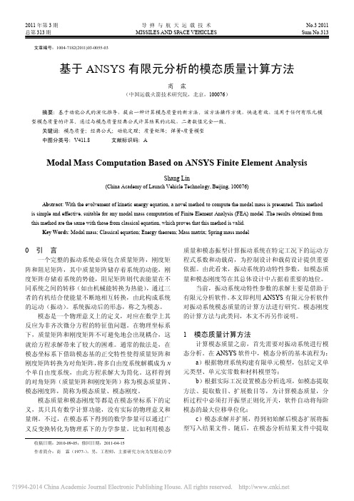
2011年第3期 导 弹 与 航 天 运 载 技 术 No.3 2011 总第313期 MISSILES AND SPACE VEHICLES Sum No.313收稿日期:2010-09-05;修回日期:2011-04-15作者简介:商 霖(1977-),男,工程师,主要研究方向为发射动力学文章编号:1004-7182(2011)03-0055-03基于ANSYS 有限元分析的模态质量计算方法商 霖(中国运载火箭技术研究院,北京,100076)摘要:基于动能公式的演化推导,提出一种计算模态质量的新方法。
该方法操作方便,快速有效,适用于任何有限元模型模态质量的计算。
通过与模态质量经典公式计算结果的比较,二者数值完全一致。
关键词:模态质量;经典公式;动能定理;质量矩阵;弹簧-质量模型 中图分类号:V411.8 文献标识码:AModal Mass Computation Based on ANSYS Finite Element AnalysisShang Lin(China Academy of Launch Vehicle Technology, Beijing, 100076)Abstract : With the evolvement of kinetic energy equation, a novel method to compute the modal mass is presented. This methodis simple and effective, suitable for any modal mass computation of Finite Element Analysis (FEA) model .The results obtained from this method are the same with those from classical equation, which proves that this method is valid.Key Words : Modal mass; Classical equation; Energy theorem; Mass matrix; Spring mass model0 引 言一个完整的振动系统必须包含质量矩阵,刚度矩阵和阻尼矩阵,其中质量矩阵储存着系统的动能,刚度矩阵存储着系统的势能,阻尼矩阵则代表能量在不同系统之间的转移(如由机械能转换为热能),通过三者的有机结合使能量不断地相互转换,由此构成系统的运动(振动)。
ANSYS实例分析-飞机机翼
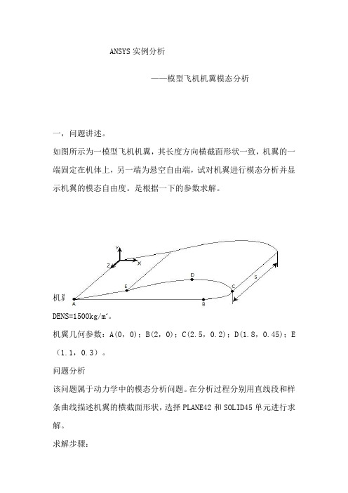
ANSYS实例分析——模型飞机机翼模态分析一,问题讲述。
如图所示为一模型飞机机翼,其长度方向横截面形状一致,机翼的一端固定在机体上,另一端为悬空自由端,试对机翼进行模态分析并显示机翼的模态自由度。
是根据一下的参数求解。
机翼材料参数:弹性模量EX=7GPa;泊松比PRXY=0.26;密度DENS=1500kg/m3。
机翼几何参数:A(0,0);B(2,0);C(2.5,0.2);D(1.8,0.45);E (1.1,0.3)。
问题分析该问题属于动力学中的模态分析问题。
在分析过程分别用直线段和样条曲线描述机翼的横截面形状,选择PLANE42和SOLID45单元进行求解。
求解步骤:第1 步:指定分析标题并设置分析范畴1.选取菜单途径Utility Menu>File>Change Title2.输入文字“Modal analysis of a model airplane wing”,然后单击OK。
3.选取菜单途径Main Menu>Preferences.4.单击Structure选项使之为ON,单击OK。
主要为其命名的作用。
第2 步:定义单元类型1.选取菜单途径:MainMenu>Preprocessor>Element Type>Add/Edit/Delete。
2.Element Types对话框将出现。
3.单击Add。
Library ofElement Types对话框将出现。
4.在左边的滚动框中单击“Structural Solid”。
5.在右边的滚动框中单击“Quad 4node 42”。
6.单击Apply。
7.在右边的滚动框中单击“Brick 8node 45”。
8.单击OK。
9.单击Element Types对话框中的Close按钮。
第3 步:指定材料性能1.选取菜单途径Main Menu>Preprocessor>MaterialProps>-Constant-Isot ropic。
制冷压缩机舌簧阀有限元分析与实验研究
摘要滚动转子压缩机是家用空调器压缩机应用中的主要机型,其采用结构简单、工作可靠的舌簧阀。
舌簧阀安装在滚动转子压缩机的排气口,通过压力启闭来控制压缩机气缸的排气,气阀性能的优劣直接影响着压缩机的性能。
目前,对于阀片性能的评价除了关注工作的稳定性外,其疲劳寿命也是一大方面。
为提高疲劳寿命,大部分厂家主要着重于消除应力集中、提高压缩残余应力、优化材料性能等几个方面。
正是在这样的背景下,开启了本课题的研究工作。
本论文主要从以下几个方面进行:首先,介绍了滚动转子压缩机的工作原理、基元容积参数以及热力参数等,点明了滚动转子压缩机重要性,间接说明了舌簧阀的应用广泛性。
其次,介绍了舌簧阀的工作原理,以MC71200110型舌簧阀为例,推导了其运动微分方程以及边界条件,并绘制了理论运动曲线;同时,针对MC71200110型舌簧阀的阀片升程、阀隙平均马赫数、阀片厚度进行设计计算。
再次,以有限元计算软件ANSYS为主要计算工具,对舌簧阀进行模态分析判断阀片与压缩机的共振情况;使用ANSYS/LS-DYNA进行动态响应分析计算,得到阀片在开启过程中的变形情况、阀片开启过程中头部某点的运动曲线、阀片撞击升程限制器的最大等效应力。
最后,分析了影响阀片寿命的因素,并指出压缩残余应力作为内在因素对阀片疲劳强度的影响以及其作用机理。
本文还搭建了一套适用于多种规格舌簧阀的加速疲劳实验台,并通过实验验证了实验台的可靠性,对阀片厂家提出阀片疲劳强度处理方面的一些建议。
关键词:滚动转子压缩机;舌簧阀;动态响应;疲劳特性;压缩残余应力ABSTRACTThe rolling rotor compressor is the main type of application of the compressor in the household air conditioner, which adopts the simple structure and reliable reed valves. The reed valve is installed on the exhaust port of the rolling piston compressor, and is controlled by pressure difference opening and closing. The property of the valve directly influences the performance of the compressor. At present, in addition to the stability of the work, the fatigue life is also a key factor for the evaluation of the performance of the valve. In order to improve the fatigue life, most of the manufacturers mainly focus on eliminating stress concentration, improving the compressive residual stress and optimizing the material performance. Just under the above context, this thesis is begun. This thesis mainly consists in the following aspects:First, introduces the working principle, basic volume parameters and thermal parameters of rolling piston compressor, points out the importance of rolling piston compressor, and the extensive application of reed valve is indirectly explained.Next, Introduces the working principle of reed valve. Taking MC71200110, a type of reed valve as an example, deduces the differential equations of motion and boundary conditions, and draw the theory of motion curve; at the same time, designs and calculates the valve lift, valve gap the average Mach number, valve plate thickness of the MC71200110.Then, using the finite element calculation software ANSYS as the main computing tool, the modal analysis of the tongue spring valve is carried out to judge the resonance of the valve plate and the compressor; using ANSYS/LS-DYNA to conduct Dynamic response analysis, obtains the deformation of valve plate during opening process, the motion curve of the head part and the maximum von stress.Finally, the factors affecting the life of the valve plate are analyzed, and the effect of the compressive residual stress on the fatigue strength of the valve plate and its mechanism of action are pointed out. This paper also provides a set of accelerated fatigue test rig for various specifications of reed valve. The reliability of the test bench is verified by experiments, and some suggestions for the valve manufacturer's fatigue strength treatment are put forward.KEYWORDS: rolling rotor compressor; reed valve; dynamic response; fatigue properties; compressive residual stress目录第1章绪论 (1)1.1课题研究背景 (1)1.1.1 滚动转子压缩机发展现状 (1)1.1.2阀片研究现状 (1)1.1.3 本文研究的意义 (2)1.2舌簧阀国内外研究现状 (2)1.3本文的主要研究内容 (3)第2章滚动转子压缩机工作过程与特点 (5)2.1 滚动转子压缩机工作原理 (5)2.2 滚动转子压缩机工作参数 (6)2.2.1 容积参数 (6)2.2.2 气缸内热力参数关系 (8)2.3滚动转子压缩机的特点 (9)2.3.1滚动转子式压缩机的优点 (9)2.3.2滚动转子式压缩机的缺点 (9)2.4本章小结 (10)第3章舌簧阀工作原理与设计 (11)3.1舌簧阀介绍 (11)3.1.1 舌簧阀工作原理 (11)3.1.2舌簧阀的运动微分方程 (15)3.1.3 排气阀片运动曲线 (12)3.2舌簧阀的工程设计 (16)3.2.1舌簧阀设计的基本要求 (16)3.2.2压缩机舌簧阀的工程设计步骤 (17)3.3 本章小结 (21)第4章基于ANSYS的舌簧阀模态分析与动态响应分析 (22)4.1 模态分析 (22)4.1.1模态分析理论 (22)4.1.2模态分析操作过程 (22)4.2舌簧阀动态响应分析 (26)4.2.1 ANSYS/LS-DYNA分析能力概述 (27)4.2.2 LS-DYNA分析的一般流程 (27)4.3 本章小结 (33)第5章阀片疲劳实验台的研制与加速疲劳实验 (34)5.1影响阀片寿命的因素 (34)5.2压缩残余应力作用影响疲劳强度机理 (34)5.3无限寿命设计理论 (35)5.4舌簧阀加速疲劳试验 (36)5.4.1加速疲劳实验原理 (36)5.4.2加速疲劳实验台的搭建 (36)5.4.3实验台系统部件 (37)5.5加速疲劳实验方案 (43)5.6实验结果分析 (44)5.7本章小结 (47)第6章总结与展望 (48)6.1总结 (48)6.2展望 (49)参考文献 (50)攻读硕士学位期间的学术活动及成果情况 (50)图2.1 制冷系统循环图 (5)图2.2滚动转子压缩机工作过程 (6)图2.3 滚动转子压缩机基元容积的几何关系 (7)图3.1 舌簧阀工程图 (11)图3.2 舌簧阀组件装配图 (11)图3.3 排气阀片边界 (13)图3.4 舌簧阀理论运动曲线 (16)图3.5三种舌簧阀有效通流面积与特征升程关系曲线 (18)图4.1 排气阀片有限元模型 (23)图4.2 阀片前十阶振型图 (25)图4.3 舌簧阀组件三维模型 (28)图4.4 网格划分 (29)图4.5 等效应力云分布图 (31)图4.6 115号节点运动曲线 (32)图5.1 压缩残余应力作用机理 (35)图5.2 加速疲劳实验台系统图 (36)图5.3 单片机控制原理图 (39)图5.4 PCB线路板 (41)图5.5 单片机控制板 (42)图5.6 MC71200110舌簧阀 (43)图5.7 X射线衍射仪 (44)图5.8 1-5号阀片残余压应力分布趋势图 (46)表3.1 阀片钢带厚度规格 (20)表4.1 阀片固有频率表 (24)表5.1 材料清单 (42)表5.2 A、B点残余应力 (44)表5.3 1~17点残余应力 (45)第1章绪论第1章绪论1.1课题研究背景随着国家经济飞速发展,使人民生活变化巨大,人们对于生活舒适度的投资不断增加。
考虑材料非线性的预应力梁模态分析

态分析,必须对该软件 自振 的计 算程序进行修正或者优化。论文 中的程 序先提取非线 性静 力计算结果中单元的应 力大小,然后
利用应力大小来修正单元的弹性模 量,通 过这种方式使得材 料的非线性特性能被ANSYS模态分析结果反映出来。
【关键 词 】 预 应 力 混凝 土 ;梁 ;模 态 分 析 ;数 值 模 拟
【中图分类号】 TU375
【文献标志码 】 A
【文章 编号】 1671-3702(2016)01—0033—05
M odal Analysis of Prestressed Beam Considering M aterial Nonlinearity ZHANG Binbin ,ZHU Yulin ,WANG Haicheng ,YAN Zhitao ,LIXiming ,WANG Qiansong
(1.National Construction Engineering Quality Supervision andInspection Center,Beijing 100013,China;
2.Chongqing University,Chongqing 400044,China) A bstract:ANSYS solved not well with material non]inear properties in the modal analysis of nonlinear materialS,SO when USing ANSYS nonlinear modal analysiS,the calculation of the software must be natural program modification or optimization. In this paper,the stress magnitude of the element was extracted from the nonlinear static calculation resultS first,and the stress magnitude of the element was used to modify the modulus of elasticity of the element,then the nonlinear characteristicS of the material could be reflected by the ANSYS modal analysiS. Keywords:prestressed concrete;beam;modal analysis:numerical simulation
ansys有限元模态分析详解

• 只能使用线性单元
• 材料可以是线性的、各向同性或各向异性的、恒定或温度相关的
• 定义的任何非线性性质均会被忽略
• 参看第一章中有关建模要考虑的因素
1-20
模态分析步骤
选择分析类型和分析选项
建模
选择分析类型和选项:
• 进入求解器并选择模态分析 • 模态提取选项* • 模态扩展选项* • 其它选项*
• ANSYS输出的是自然频率fi ,而不是圆频率i 。 • 特征向量 {u}i 表示振型, 即假定结构以频率 fi振动时的形状
1-6
模态分析
… 术语与概念(接上页)
培训手册
• 模态提取 是用来描述特征值和特征向量计算的术语。
• 模态扩展有两重含义。对于缩减法,模态扩展是从缩减模态形式计算全 模态形式;对于其它的方法,模态扩展仅仅是表示把模态形式写入结果 文件。
1-18
模态分析
C. 步骤
模态分析中的四个主要步骤: • 建模 • 选择分析类型和分析选项 • 施加边界条件并求解 • 评价结果
培训手册
1-19
ANSYS80模态分析——段志东制作
ANSYS80模态分析——段志东制作
模态分析步骤
建模
培训手册
• 必须定义杨氏模量(或某种形式的刚度)和密度(或某种质量形式)
• 什么是模态分析?
– 模态分析可以用来确定研究对象的振动特性,是其它动力学分析的起点。
• 定义结构振动特性的方法:
– 固有频率 – 模态形式 – 模态参与因子(在特定方向上某个模态的参与的程度)
• 模态分析是各种动力学分析类型最基础的内容。
1-3
ANSYS80模态分析——段志东制作
模态分析
… 定义和目的
ANSYS模态分析实例教程文件

8
9. 对于Y 和Z 方向,输入0替换“Free”, “X” 方向仍 然保留为 “Free”.
Workshop Supplement
9
July 10, 2007 © 2007 ANSYS, Inc. All rights reserved.
ANSYS, Inc. Proprietary
Inventory #002406 WS1-8
ANSYS, Inc. Proprietary
Inventory #002406 WS1-4
Workbench-Simulation Dynamics
Workshop 1 – 设置
1. 当导入几何模型之后,从“Map of Analysis Types”选择“Static Structural”。
• 目的在于计算某一悬索桥模型的振动特性
– 塔科马海峡大桥,又称为“ Galloping Gertie”,因其在1940年出任意 外的倒塌而出名。
• 在该实例中,首先对桥的模型进行分析,然后计算大桥的固有频 率和固有振型。
• 在求解中,我们考虑到了结构的“预应力”,因为自重载荷预先 作用于桥梁上而导致拉索产生了预拉力,从而增加了整体刚度。
Inventory #002406 WS1-3
Workbench-Simulation Dynamics
Workshop 1 – 起始页
• 从“ WorkBench Project Launcher ”点击“ Simulation”。
–
如果进入“Simulation” ,点击 >File>New
•
Inventory #002406 WS1-6
Workbench-Simulation Dynamics
- 1、下载文档前请自行甄别文档内容的完整性,平台不提供额外的编辑、内容补充、找答案等附加服务。
- 2、"仅部分预览"的文档,不可在线预览部分如存在完整性等问题,可反馈申请退款(可完整预览的文档不适用该条件!)。
- 3、如文档侵犯您的权益,请联系客服反馈,我们会尽快为您处理(人工客服工作时间:9:00-18:30)。
ANSYS EXERCISEModal Analysis of a Spring-Mass SystemCopyright 2001-2002, John R. BakerIn this exercise, you will solve for the natural frequencies and mode shapes of the 2-DOF system shown below. Step-by-step instructions are provided beginning on the following page.If you run into problems with these instructions, feel free to contact:John Baker; Phone: 270-534-6342; Email: jbaker@Notes: ANSYS has an option that will allow for the masses to be modeled as point masses. Using this option, no dimensions or material properties would be necessary for the masses. However, so that the mode shapes are easier to understand when they are animated, in this case, the masses will be modeled as blocks, 1 m x 1 m, with unit thickness. So, they have a volume of 1 m 3. The densities will be specified to produce the correct masses. Also, the free lengths of the springs are irrelevant in this analysis, as only the stiffnesses matter. But, they will both be assumed to have a length of 5 m.M=2 kg x 1x 2K =5 N/m K =20 N/m M=1 kgThe steps that will be followed, after launching ANSYS, are:Preprocessing:1. Change jobname.2. Define element types (#1 - Solid42 element; #2 - Combin14 element).3. Specify material properties for the masses.4. Specify real constants for the springs. (Spring stiffnesses.)5. Create rectangles (actually, “squares”)6. Specify mesh controls for the masses.7. Mesh the areas.8. Create a node at the wall.9. Create the spring elements.10. Apply constraints.11. Make rigid body constraints for each mass.Solution:12. Specify analysis type and options.13. Solve.Postprocessing:14. List the natural frequencies.15. Animate the mode shapes.16. List the mode shapes.Exit17. Exit the ANSYS program, saving all data._____________________________________________________________________________ Launching ANSYS:It is probably best to save your work on a Zip Disk in the computer IOMEGA Zip Drive. On any machine in the computer lab (on the first floor of Crounse Hall), insert a Zip Disk in the drive. Then, simply click on the ANSYS icon on the Windows Desktop. The ANSYS Launcher menu should appear. It is shown at the top of the next page. The only input you will likely need on this menu is specification of the Zip Drive as your “Working Directory”. If you don’t have a Zip Disk, or if you prefer to work on the computer hard drive instead, then specify any directory (or, “Folder”) as your working directory. To browse and find the desired wo rking directory, click on the button with the three dots to the far right on the Launcher Menu on the line that says “Working Directory”. Once the working directory is specified, click on “Run” at the bottom of the Launcher Menu.The ANSYS menus should open up. You will see a Main Menu, illustrated on the following page, and a large black graphics window. You are now ready to begin creating the model and performing the analysis.ANSYS Launcher Menu:ANSYS Main Menu:Note: Most of the required tasks are performed using menu picks from the ANSYS Graphical User Interface, as specified in italics in the step-by-step instructions below. It is sometimes more convenient, however, to enter certain commands directly at the command line. The command line is seen on the screen as:The method of direct command line entry is used in some cases in this exercise, whenever this method is more convenient than using menu picks.Often, as an alternative, an input fi le, known as a “batch file”, is created, which is simply an ASCII text file containing a string of ANSYS commands in the appropriate order. ANSYS can read in this file as if it were a program, and perform the analysis in “batch mode”, without ever opening up the Graphical User Interface. The batch file option is not covered in this exercise.****IMPORTANT***: AS YOU WORK THROUGH THIS EXERCISE, WITHIN ANSYS, ON THE ANSYS TOOLBAR (UPPER RIGHT), CLICK ON “SAVE_DB” OFTEN!!! THIS TOOLBAR APPEARS AS:At any point, if you want to resume from the previous time the model was saved, simply click on “RESUM_DB” on this same Toolbar. Any information entered since the last save will be lost, but this is a nice feature in the event that you make an input mistake, and are unsure of how to correct it.There are a number of ways to model a system and perform an analysis in ANSYS. The steps below present only one method.Preprocessing:1. Change jobname. On the Utility Menu across the very top of the screen, select:File -> Change JobnameEnter “modalsys1”, and click on “OK”.2. Define element types:Preprocessor -> Element Type -> Add/Edit/DeleteClick on “Add”. The “Library of Element Types” box appears, as shown. Scroll down to highlight “Solid”, and “Quad 4node 42” as shown. Click on “APPLY”.Now, scroll down to highlight “Combination” and “Spring-Damper 14” as shown, then click on “OK” and “Close”.3. Specify material properties for the masses:Preprocessor -> Material Props -> -Constant- IsotropicOn the box, shown on the next page, enter “1” in the “EX” input field (EX is the modulus of elasticity), and enter “2” in the “DENS” input field, as shown, then click on “APPLY”.Note that an arbitrary value was entered for EX, because we will couple all DOF on eachmass so that they move as rigid bodies. So, the modulus of elasticity for each mass, in this particular analysis, is irrelevant. However, we chose the density to produce a block of mass=2 kg. Our block will have a volume of 1 m3.After entering the input, click on “APPLY”. The “Isotropic Materials Box” should be showing on the screen, and at this point, the material number is still set to “1”. Change the material number to “2”, and click on “OK”. The mater ial properties box, like that below, re-opens. Again, enter “1” for EX, but this time, enter “1” for density. Click on “OK”.4. Specify real constants for the springsPreprocessor -> Real Constants -> Add/Edit/Delete -> AddThe box below will open. Be sure that “Type 2 COMBIN14” is highlighted, and click on “OK”For real constant set “1”, choose “K=5”, as shown below. Leave the other fields blank, and click on “Apply”. Then, change the Set Number to “2”, and enter a value of “20”for K, the n click on “OK”, then “Close”. Note that, for this model, we will not need any real constants for the PLANE42 elements. We are using the option that assumes a unit thickness for these elements.5. Create rectangles:Preprocessor -> Modeling- Create -> -Areas- Rectangle -> By DimensionsFill in (X1,X2)=(5,6), and (Y1,Y2)=(0,1), as shown below. Then, click on “Apply”.Create the block for the other mass by filling in (X1,X2)=(11,12), and (Y1,Y2)=(0,1), and then click “OK”.6. Specify mesh controls for the masses.As stated previously, this model involves creating blocks to model the masses, but they are going to be set so that each mass moves as a rigid body. In general, in finite element modeling, the finer the mesh, the more accurate the results. However, in this case, the mesh density for each separate mass is irrelevant. So, each mass will be modeled as a single element. Choose:Preprocessor -> -Meshing- Size Cntrls -> -Lines- Picked LinesThis opens up a Picking Menu, as shown on the next page. This box would allow for picking individual lines. But, in this case, we want a single element division for every line. So, in the Picking Menu, choose “Pick All”. This opens up an “Element Sizes”box, also shown on the next page. Input “1” for “NDIV” , as shown, and click on “OK”.7. Mesh the areas.First, in case the areas are not currently plotted, along the top toolbar:Choose: Plot -> AreasThen, choose:Preprocessor -> -Meshing- Mesh -> -Areas- Mapped -> 3 or 4 sidedA Picking Menu opens (which has the label “Mesh Areas” at the top of the menu).Click on the block on the left (which will be the 2 kg mass). It should highlight. Then, click on “OK” in the Picking Menu. Since we are only creatin g a single element in each block, at this point, a plot of the elements looks just like a plot of the areas. But, there are now nodes at the corners of the left-hand block, and this block contains a single PLANE42 finite element. Probably, an element plot has appeared showing only the single meshed element.Re-plot the areas, as done above, by choosing, on the top toolbar: Plot -> AreasNow, before meshing the second area, the material number needs to be changed to number 2, because the density of the two masses is different, and we defined different materials to account for this. To do this, use the path:Preprocessor -> -Modeling- Create -> Elements -> Elem AttributesThe box below opens. Change the [MAT] entry to “2”, as shown. No other chan ges are needed at this time, so click “OK”.Now, to mesh the second mass, choose:Preprocessor -> -Meshing- Mesh -> -Areas- Mapped -> 3 or 4 sidedA Picking Menu opens (which has the label “Mesh Areas” at the top of the menu).Click on the block on the right (which will be the 1 kg mass). It should highlight. Then, click on “OK” in the Picking Menu.8. Create a node at the wall:Preprocessor –> Create -> Nodes -> In Active CSIn the box that opens, as shown on the next page, there is no input required for this case. This is only because we are going to create the node at (X,Y,Z)=(0,0,0). Also, we do not need a node number, because ANSYS will use the lowest available node number if we leave the node number field blank. Just click on “OK”.It is probably a good idea now to turn off the display of the X-Y-Z triad, because it covers up the node at the wall in the plots. Along the top toolbar:Choose: PltCtrls -> Window Controls -> Window Options.In the box that opens, for [/TRIAD], select “Not shown”, then click on “OK”.Now, it is probably a good idea to turn the node numbers on. They may be showing already at this time, but to make sure they are, on the top toolbar:Back on the top toolbar, again choo se “PlotCtrls”, then “Numbering”, and the box below opens. Toggle the “Node” option from “Off” to “On” by clicking on the box. You should see a check mark appear in the box, as shown below.Although nodes are probably already plotted now, to make sure, on the top toolbar, choose Plot -> Nodes.9. Create the spring elements.First, the element type needs to be changed to type 2, which is the element type number we used in defining the Combin14 (spring) element type. To do this, use the path:Preprocessor -> -Modeling- Create -> Elements -> Elem AttributesThe box below opens. Change the [TYPE] entry to “2 COMBIN14” as shown. No other changes are needed at this time, so click “OK”.Now, to create the first spring element, choose:Preprocessor -> -Modeling- Create -> Elements -> -Auto Numbered –Thru NodesA picking menu opens. It should be that the numbered nodes are plotted on screen at thistime. Node number 9 should be the node at the wall, and node number 1 should be the node at the bottom left-hand side of the 2 kg mass.Click once, with the left mouse button, on node 9, then click again, once, on node 1.Then, in the picking menu, click on “OK”.Now, before creating the other spring, the real constant set number needs to be changed to set 2, because the spring constant is different for the two springs. To do this, use the path:Preprocessor -> -Modeling- Create -> Elements -> Elem AttributesIn the box that opens, change the [REAL] entry to “2”. No other cha nges are needed at this time, so click “OK”. Then, choose:Preprocessor -> -Modeling- Create -> Elements -> -Auto Numbered –Thru NodesA picking menu opens. Node number 2 should be the node at the bottom-right corner ofthe left-hand mass, and node 5 should be the node at the bottom-left corner of the right-hand mass. Click once, with the left mouse button, on node 2, then click again, once, on node 5. Then, in the picking menu, click on “OK”.Plot the elements, by choosing, on the top toolbar: Plot-> Elements10. Apply constraints.It is assumed that only X-direction motion is allowed. So, the Y and Z direction motion must be constrained to zero at all nodes.Preprocessor -> Loads -> Apply -> Displacement -> On NodesA picking menu applies. We want this constraint to apply to all nodes in the model. So,in the picking menu, choose “Pick All”. Another box opens. Be sure to Un-highlight“All DOF”, by clicking on it. Then, highlight “UY” and “UZ” by clicking on these labels, as shown, and then click on “Apply”.The picking menu should remain open. Click on the node at the wall (this should be node number 9), and then click on “OK” in the Picking Menu. This node should not move in any direction. So, choose, in the box that opens, as shown on the previous page, click on “All DOF”, and then click on “OK”.11. Make rigid body constraints for each mass.Each mass is supposed to move as a rigid body. We can produce this effect by coupling all nodes on each mass so that they move together. To do this, choose:Preprocessor -> Coupling / Ceqn -> Couple DOFsA picking menu opens. Click on nodes 1-2-3-4, to highlight all four nodes that define theleft-hand mass. Then, in the Picking Menu, click on “Apply”. A box, as shown below, o pens. Enter “1” for “NSET”, as shown, and leave the label “UX” for “Lab”. Then, click on “Apply”.The picking menu should re-open. Click on nodes 5-6-7-8, to highlight all four nodes that define the right-hand mass. Then, in the Picking Menu, click o n “OK”. A box, as shown above, re-opens. This time, Enter “2” for “NSET”, and again leave the label “UX” for “Lab”. Then, click on “OK”.12. Specify analysis type and options.Return to the main ANSYS Menu, and choose:Solution -> -Analysis Type- New AnalysisIn the box that opens, select “Modal” and click on “OK”.Then, select: Solution -> Analysis OptionsThe box below opens. Enter “2” for “No. of modes to extract” and “2” for “NMODE No. of modes to expand”. Choose “OK”, and the box at bottom opens. Enter “1000” for “FREQE”, as shown, then click on “OK”.13. SolveChoose: Solution -> -Solve- Current LSA green box will appear. Just click on “OK” in the box. You should then, very quickly,get a yellow box, with the note “Solution is done!”. You can close this box.14. List Natural FrequenciesReturn to the ANSYS Main Menu, and choose:General Postproc -> Results SummaryYou should get a box listing two natural frequencies. One is for “Set 1” and the other is for “Set 2”. Set 1 is the set of results corresponding to Mode 1, and Set 2 is the set of results corresponding to Mode 2. Note the natural frequencies (these are listed in units of “Hz”), then close the listing box.15. Animate the Mode ShapesChoose: General Postproc -> -Read Results- First SetThen, on the top toolbar, choose: PlotCtrls -> Animate -> Mode ShapeIn the box that opens, you may want to change “No. of frames to create” to some higher number than the default of 10. For instance, you may enter 20. Also, you may want to change the time delay to some smaller number than the default of 0.5. For instance, you may enter 0.2. Then, in that box, click on “OK”.It may take a couple of minutes for the animation to begin, but eventually, you should see, on the screen, the expected motion corresponding to the first mode shape. At any time, you can click on “Close” in the blue “Animation Controller” box to end the animation.To animate the second mode shape, choose:General Postproc -> -Read Results- Next SetAgain, back on the top toolbar, choose: PlotCtrls -> Animate -> Mode ShapeRepeat the procedure outlined above, and you should see the animation of the second mode shape.16. List the Mode ShapesChoose: General Postproc -> -Read Results- First SetThen, choose: General Postproc -> List Results -> Nodal SolutionIn the box that opens, as shown below, keep the defaults by just clicking on “OK”.A listing of the relative displacements for each node for mode 1 is shown, and thefrequency for the mode is also shown.You can get a hard copy of the information in this box by clicking, in this listing box: File -> Print. It should also be possible to save this information to a file using the option, File -> Save As. However, this “Save As” option does not appear to be working properly in the current ANSYS version. Another option, however, is to use the mouse to block this information in (hold down left mouse button and drag to highlight the text and numbers), then, on the keyboard, sim ultaneously hit the Control Key, and the letter “c”(Ctrl-C), then, open up either “Notepad”, or some word processing program, such as Microsoft Word. In the program of your choosing, choose “Paste”, or else use “Ctrl-V”, to insert the text copied from the listing box. If desired, you may close the listing box to get it out of the way. To do this, in that listing box, choose: File -> Close.Now, list the second mode shape in a similar way. First, choose:General Postproc -> -Read Results- Next SetThen, as above, choose: General Postproc -> List Results -> Nodal SolutionIn the box that opens, choose “OK”. You can again get either a hard copy print-out of the information, or save it in a file, as outlined above.17. Exit the ANSYS program, saving all data.On the ANSYS Toolbar, shown below, choose:Quit ->Save Everything -> OKTo recall the model and solution at a later date, assuming you have deleted no files, simply re-launch ANSYS, specify the same working directory as before, re-issue the same jobname as used in Step 1 of these instructions, and then click on “RESUME_DB” on the ANSYS Toolbar shown above.To see the resumed model in the graphics window, you may then need to click on “Plot” on the top Utility Menu:T hen, choose either “Elements”, “Nodes”, or “Areas”, depending on which entities you wish to plot.。